Lang-Firsov approaches to polaron physics: From variational methods to unbiased quantum Monte Carlo simulations

1 Introduction

In the last decades, there has been substantial interest in simple models for electron-phonon (el-ph) interaction in condensed matter. Despite intensive theoretical efforts, it was not before the advent of numerical methods in the 1980’s that a thorough understanding on the basis of exact, unbiased results was achieved. Although at the present our knowledge of the rather simple cases of a single carrier (the polaron problem) or two carriers (the bipolaron problem) in Holstein and Fröhlich models is fairly complete, this is not true for arbitrary band fillings. There is still a major desire to develop more efficient simulation techniques to tackle strongly correlated many-polaron models, which are expected to describe several aspects of real materials currently under investigation, such as quantum dots and quantum wires, high-temperature superconductors or colossal-magnetoresistance manganites.

One of the principle problems in computer simulations of microscopic models is the limitation in both system size and parameter values. Whereas the former can be overcome for the polaron and the bipolaron problem in some cases, it is very difficult to obtain results of similar quality in the many-electron case. Moreover, many approaches still suffer from severe restrictions concerning the parameter regions accessible. For example, interesting materials such as the cuprates and manganites are characterized by small but finite phonon frequencies—as compared to the electronic hopping integral—and intermediate to strong el-ph interaction. Unfortunately, simulations turn out to be most difficult exactly for such parameters, and it is therefore highly desirable to improve existing simulation methods.

In this chapter, we shall mainly review different versions of a recently developed quantum Monte Carlo (QMC) method applicable to Holstein-type models with one, two or many electrons. The appealing advantages of QMC over other numerical methods include the accessibility of rather large systems, the exact treatment of bosonic degrees of freedom (i.e., no truncation is necessary), and the possibility to consider finite temperatures to study phase transitions. The important new aspect here is the use of canonically transformed Hamiltonians, which permits the introduction of exact sampling for the phonon degrees of freedom, enabling us to carry out accurate simulations in practically all interesting parameter regimes.

Additionally, based on a generalization of the Lang-Firsov transformation, we shall present a simple variational approach to the polaron and the bipolaron problem which yields surprisingly accurate results.

The chapter is organized as follows. In section 2, we present the general model Hamiltonian. Section 3 is devoted to a discussion of the Lang-Firsov transformation, and section 4 contains the derivation of the variational approach. The QMC method is introduced in section 5. Section 6 gives a selection of results for the cases of one, two and many electrons. Finally, we summarize in section 7.

2 Model

In this paper we focus on the extended Holstein-Hubbard model defined by

$$H= - t\sum_{\langle ij\rangle\sigma}c^{\dagger}_{i\sigma}c_{j\sigma}+U\sum_{i}\widehat{n}_{i\uparrow}\widehat{n}_{i\downarrow}+V\sum_{\langle ij\rangle}\widehat{n}_{i}\widehat{n}_{j}$$ (1)

$$+ \frac{\omega_{0}}{2}\sum_{i}(\widehat{p}^{2}_{i}+\widehat{x}^{2}_{i})-g^{\prime}\sum_{i}\widehat{n}_{i}\widehat{x}_{i}\,.$$

Here $c^{\dagger}_{i\sigma}$ creates an electron with spin $\sigma$ at site $i$, and $\widehat{n}_{i}=\sum_{\sigma}\widehat{n}_{i\sigma}$ with $\widehat{n}_{i\sigma}=c^{\dagger}_{i\sigma}c^{\phantom{{\dagger}}}_{i\sigma}$. The phonon degrees of freedom at site $i$ are described by the momentum $\widehat{p}_{i}$ and coordinate (displacement) $\widehat{x}_{i}$ of a harmonic oscillator. The microscopic parameters are the nearest-neighbour (denoted by $\langle\rangle$) hopping amplitude $t$, the on-site (Hubbard–) repulsion $U$, the nearest-neighbour Coulomb repulsion $V$, the Einstein phonon frequency $\omega_{0}$ and the el-ph coupling $g^{\prime}$.

This model neglects both long-range Coulomb and el-ph interaction, which is often a suitable approximation for metallic systems due to screening. Two simple limiting cases of the Hamiltonian (1) are the Holstein model ($U=V=0$) and the Hubbard model ($g^{\prime}=V=0$). In general, the physics of the model (1) is determined by the competition of the various interactions. Depending on the choice of parameters and band filling, it describes fascinating phenomena such as (bi-)polaron formation, Mott– and Peierls quantum phase transitions or superconductivity. As we shall see below, the adiabaticity ratio

$$\alpha=\omega_{0}/t$$ (2)

permits us to distinguish two physically different regimes, namely the adiabatic regime $\alpha<1$ and the non-adiabatic regime $\alpha>1$.

We further define the dimensionless el-ph coupling parameter $\lambda=g^{\prime 2}/(\omega_{0}W)$, where $W=4t\mathrm{D}$ is the bare bandwidth in D dimensions. Alternatively, $\lambda$ may also be written as $\lambda=2E_{\text{P}}/W$, i.e., the ratio of the polaron binding energy in the atomic limit $t=0$, $E_{\text{P}}=g^{\prime 2}/2\omega_{0}$, and half the bare bandwidth. A useful constant in the non-adiabatic regime is $g^{2}=E_{\text{P}}/\omega_{0}$. We exclusively consider hypercubic lattices with linear size $N$ and volume $N^{\mathrm{D}}$, and assume periodic boundary conditions in real space.

3 Lang-Firsov transformation

The cornerstone of the methods presented here is the canonical (extended) Lang-Firsov transformation of the Hamiltonian (1). The original Lang-Firsov (LF) transformation LangFirsov has been used extensively to study Holstein-type models. A well-known, early approximation is due to Holstein Ho59a , who replaced the hopping term by its expectation value in a zero-phonon state, neglecting emission and absorption of phonons during electron transfer. However, this approach yields reliable results only in the non-adiabatic strong-coupling (SC) limit. For $\lambda=\infty$ (or $t=0$), the LF transformation provides an exact solution of the single-site problem Ma90 .

Whereas transformed Hamiltonians have been treated numerically before dMeRa97 ; Robin97 ; FeLoWe00 , the first QMC method making use of the LF transformation has been proposed in HoEvvdL03 .

We introduce the extended LF transformation by defining the unitary operator

$$\widehat{\Phi}=\mathrm{e}^{S}\,,\quad S=\mathrm{i}\sum_{ij}\gamma_{ij}\widehat{n}_{i}\widehat{p}_{j}$$ (3)

with real parameters $\gamma_{ij}$, $i,j=1,\dots,N^{\mathrm{D}}$. $\widehat{\Phi}$ as defined in equation (3) has the form of a translation operator, and fulfills $\widehat{\Phi}^{\dagger}=\widehat{\Phi}^{-1}$. Given an electron at site $i$, $\widehat{\Phi}$ mediates displacements $\gamma_{ij}$ of the harmonic oscillators at all sites $j$. Hence, the extended transformation is capable of describing an extended phonon cloud, important in the large-polaron or bipolaron regime. We shall use this transformation for the variational approach. However, the standard (local) LF transformation will be expedient as a basis for unbiased QMC simulations, in which the transformed Hamiltonian is treated exactly.

Operators have to be transformed according to $\widetilde{\widehat{A}}=\widehat{\Phi}\widehat{A}\widehat{\Phi}^{\dagger}$. Defining the function $f(\eta)=\mathrm{e}^{\eta\widehat{S}}\widehat{A}\mathrm{e}^{-\eta\widehat{S}}$ we obtain

$$f^{\prime}(\eta)=\mathrm{e}^{\eta\widehat{S}}[\widehat{S},\widehat{A}]\mathrm{e}^{-\eta\widehat{S}}\,,$$ (4)

where $f^{\prime}\equiv\partial f/\partial\eta$. A simple calculation gives

$$[\widehat{S},c_{i\sigma}]=-\mathrm{i}\sum_{l}\gamma_{il}\,\widehat{p}_{l}\,c_{i\sigma}\,,\quad[\widehat{S},c^{\dagger}_{i\sigma}]=\mathrm{i}\sum_{l}\gamma_{il}\,\widehat{p}_{l}\,c^{\dagger}_{i\sigma}\,.$$ (5)

Substitution in equation (4), integration with respect to $\eta$ and setting $\eta=1$ results in

$$\widetilde{c}_{i\sigma}^{\dagger}=c_{i\sigma}^{\dagger}\,\mathrm{e}^{\mathrm{i}\sum_{j}\gamma_{ij}\widehat{p}_{j}}\,,\qquad\widetilde{c}_{i\sigma}=c_{i\sigma}\,\mathrm{e}^{-\mathrm{i}\sum_{j}\gamma_{ij}\widehat{p}_{j}}\,.$$ (6)

For phonon operators, the relation

$$\widetilde{\widehat{A}}=\mathrm{e}^{\widehat{S}}\widehat{A}\mathrm{e}^{-\widehat{S}}=\widehat{A}+[\widehat{S},\widehat{A}]+\frac{1}{2!}[\widehat{S},[\widehat{S},\widehat{A}]]+\cdots\,,$$ (7)

yields

$$\widetilde{\widehat{x}}_{i}=\widehat{x}_{i}+\sum_{j}\gamma_{ij}\widehat{n}_{j}\,,\qquad\widetilde{\widehat{p}}_{i}\;={\widehat{p}}_{i}\,.$$ (8)

Collecting these results, the transformation of the Hamiltonian (1) leads to

$$\widetilde{H} = \underbrace{-t\sum_{\langle ij\rangle\sigma}c^{\dagger}_{i\sigma}c^{\phantom{{\dagger}}}_{j\sigma}\mathrm{e}^{\mathrm{i}\sum_{l}(\gamma_{il}-\gamma_{jl})\widehat{p}_{l}}}_{\widetilde{H}_{\text{kin}}}+\underbrace{\frac{\omega_{0}}{2}\sum_{\phantom{\langle\rangle}i\phantom{\langle\rangle}}(\widehat{p}^{2}_{i}+\widehat{x}^{2}_{i})}_{\widetilde{H}_{\text{ph}}\equiv\widetilde{H}_{\text{ph}}^{p}+\widetilde{H}_{\text{ph}}^{x}}+\underbrace{\sum_{ij}\widehat{n}_{j}\widehat{x}_{i}(\omega_{0}\gamma_{ij}-g^{\prime}\delta_{ij})}_{\widetilde{H}_{\text{ep}}}$$ (9)

$$+\underbrace{\sum_{ij}\widehat{n}_{i}\widehat{n}_{j}\left(\frac{\omega_{0}}{2}\sum_{l}\gamma_{lj}\gamma_{li}-g^{\prime}\gamma_{ij}+\frac{U}{2}\delta_{ij}+V\delta_{\langle ij\rangle}\right)-\mbox{\small$\frac{1}{2}$}U\sum_{i}\widehat{n}_{i}}_{\widetilde{H}_{\text{ee}}}.$$

Here the term $\widetilde{H}_{\text{ep}}$ describes the coupling between electrons and phonons, whereas $\widetilde{H}_{\text{ee}}$ represents an effective el-el interaction. Hamiltonian (9) will be the starting point for the variational approach in section 4.

For QMC simulations, it is more suitable to require that the el-ph terms in $\widetilde{H}_{\mathrm{ep}}$ cancel. This can be achieved by setting $\gamma_{ij}=\gamma\delta_{ij}$ with

$$\gamma=\sqrt{\frac{\lambda W}{\omega_{0}}}\,.$$ (10)

The parameter $\gamma$ corresponds to the distortion which minimizes the potential energy of the shifted harmonic oscillator $E_{\text{pot}}=\frac{\omega_{0}}{2}x^{2}-g^{\prime}x$. This leads us to the standard LF transformation

$$\widehat{\Phi}_{0}=\mathrm{e}^{S_{0}}\,,\quad S_{0}=\mathrm{i}\gamma\sum_{i}\widehat{n}_{i}\widehat{p}_{i}\,,$$ (11)

and the familiar results for the transformed operators

$$\widetilde{c}^{\dagger}_{i\sigma}=c^{\dagger}_{i\sigma}\mathrm{e}^{\mathrm{i}\gamma\widehat{p}_{i}}\,,\qquad\widetilde{c}_{i\sigma}=c_{i\sigma}\mathrm{e}^{-\mathrm{i}\gamma\widehat{p}_{i}}$$ (12)

and

$$\widetilde{\widehat{x}}_{i}=\widehat{x}_{i}+\gamma\widehat{n}_{i}\,,\qquad\widetilde{\widehat{p}}_{i}=\widehat{p}_{i}\,.$$ (13)

In contrast to the non-local transformation (3), only the oscillator at the site of the electron is displaced. The transformed Hamiltonian reads

$$\widetilde{H} = \underbrace{-t\sum_{\langle ij\rangle\sigma}c^{\dagger}_{i\sigma}c^{\phantom{{\dagger}}}_{j\sigma}\mathrm{e}^{\mathrm{i}\gamma(\widehat{p}_{i}-\widehat{p}_{j})}}_{\widetilde{H}_{\text{kin}}}+\underbrace{\frac{\omega_{0}}{2}\sum_{\phantom{\langle\rangle}i\phantom{\langle\rangle}}(\widehat{p}^{2}_{i}+\widehat{x}^{2}_{i})}_{\widetilde{H}_{\text{ph}}}$$ (14)

$$+\underbrace{(\mbox{\small$\frac{1}{2}$}U-E_{\text{P}})\sum_{i}\widehat{n}_{i}^{2}+V\sum_{\langle ij\rangle}\widehat{n}_{i}\widehat{n}_{j}-\mbox{\small$\frac{1}{2}$}U\sum_{i}\widehat{n}_{i}}_{\widetilde{H}_{\text{ee}}}\,.$$

As we shall discuss in detail in section 5, the difficulties encountered in QMC simulations of the original Hamiltonian (1) are to a certain extent related to (bi-)polaron effects, i.e., to the dynamic formation of spatially rather localized lattice distortions which surround the charge carriers and follow their motion in the lattice.

For a single electron, the aforementioned Holstein-Lang-Firsov (HLF) approximation Ho59a becomes exact in the non-adiabatic SC or small-polaron limit, and agrees qualitatively with exact results also in the intermediate-coupling (IC) regime ZhJeWh99 . Although it overestimates the shift $\gamma$ of the equilibrium position of the oscillator in the presence of an electron, and does not reproduce the retardation effects when the electron hops onto a previously unoccupied site, the approximation mediates the crucial impact of el-ph interaction on the lattice. Consequently, the transformed Hamiltonian (14) can be expected to be a good starting point for QMC simulations, which then merely need to account for the rather small fluctuations around the (shifted or unshifted) equilibrium positions. In principle, it would also be possible to develop a QMC algorithm based on the Hamiltonian (9)—the basis of our variational approach—with the parameters $\gamma_{ij}$ determined variationally, but the local LF transformation proves to be sufficient.

The Hamiltonian (14) does no longer contain a term coupling the electron density $\widehat{n}$ and the lattice displacement $\widehat{x}$. By contrast, the extended transformation does not eliminate the interaction term completely. On top of that, the hopping term involves all phonon momenta $\widehat{p}_{i}$ as well as the parameters $\gamma_{ij}$, and the el-el interaction becomes long ranged [cf equation (9)].

For spin dependent carriers with $\widehat{n}_{i}^{2}\neq\widehat{n}_{i}$, the interaction term $\widetilde{H}_{\text{ee}}$ contains a Hubbard-like attractive interaction. Whereas the latter can be treated exactly in the case of two electrons (section 5.1), the many-electron case requires the introduction of auxiliary fields which complicate simulations. However, no such difficulties arise for the spinless Holstein model considered in section 6.

4 Variational approach

For simplicity, we shall restrict the following derivation to one dimension; an extension to $\mathrm{D}>1$ is straight forward. Furthermore, we only consider finite clusters with periodic boundary conditions, although infinite systems may also be treated. The results of this section have originally been presented in HoEvvdL03 ; HovdL05 .

4.1 One electron

As noted before, the simple variational method presented here is based on the extended transformation (3), leading to the Hamiltonian (9). We treat the $\gamma_{ij}$ as variational parameters which are determined by minimizing the ground-state energy in a zero-phonon basis in which $\langle\widetilde{H}_{\mathrm{ep}}\rangle=0$.

For systems with translation invariance the displacement fields satisfy the condition $\gamma_{ij}=\gamma_{|i-j|}$. Together with $\sum_{i}\widehat{n}_{i}=1$ for a single electron we get $\widetilde{H}_{\text{ee}}=\frac{\omega_{0}}{2}\sum_{l}\gamma^{2}_{l}-g^{\prime}\gamma_{0}$.

The eigenvalue problem of the transformed Hamiltonian (9) is solved by making the following ansatz for the one-electron basis states

$$\left\{\left|l\right\rangle=c^{\dagger}_{l\sigma}\left|0\right\rangle\otimes\prod_{\nu=1}^{N}|\phi_{0}^{(\nu)}\rangle\,,\quad l=1,\dots,N\right\}\,,$$ (15)

where $|\phi_{0}^{(\nu)}\rangle$ denotes the ground state of the harmonic oscillator at site $\nu$. The non-zero matrix elements of the hopping term are

$$\left\langle l\right|\widetilde{H}_{\text{kin}}\left|l^{\prime}\right\rangle = -t\delta_{\left\langle ll^{\prime}\right\rangle}\prod_{\nu}\langle\phi^{(\nu)}_{0}|\mathrm{e}^{\mathrm{i}(\gamma_{l\nu}-\gamma_{l^{\prime}\nu})\widehat{p}_{\nu}}|\phi^{(\nu)}_{0}\rangle$$ (16)

$$= -t\delta_{\left\langle ll^{\prime}\right\rangle}\;\prod_{\nu}\;\int\,\mathrm{d}x\,\phi(x+\gamma_{l\nu})\phi(x+\gamma_{l^{\prime}\nu})$$

$$= -t\delta_{\left\langle ll^{\prime}\right\rangle}\mathrm{e}^{-\frac{1}{4}\sum_{\nu}(\gamma_{\nu}-\gamma_{\nu+l-l^{\prime}})^{2}}\,,$$

where $\phi(x)$ denotes the real-space wavefunction of the harmonic-oscillator ground state. The Kronecker symbol $\delta_{\left\langle ll^{\prime}\right\rangle}$ forces $l$ and $l^{\prime}$ to represent nearest-neighbor sites. A simple calculation gives for the other terms in equation (9)

$$\left\langle l\right|\widetilde{H}_{\text{ph}}\left|l^{\prime}\right\rangle=\delta_{ll^{\prime}}\frac{\omega_{0}}{2}\,,\,\,\,\left\langle l\right|\widetilde{H}_{\text{ep}}\left|l^{\prime}\right\rangle=0\,,\,\,\,\left\langle l\right|\widetilde{H}_{\text{ee}}\left|l^{\prime}\right\rangle=\delta_{ll^{\prime}}\left(\frac{\omega_{0}}{2}\sum_{l}\gamma_{l}^{2}-g^{\prime}\gamma_{0}\right).$$ (17)

In the zero-phonon subspace spanned by the basis states (15), the eigenstates of Hamiltonian (9) with momentum $k$ are

$$|\psi_{k}\rangle=c^{\dagger}_{k\sigma}\left|0\right\rangle\otimes\prod_{\nu}|\phi_{0}^{(\nu)}\rangle$$ (18)

with eigenvalues

$$E(k)=E_{\text{kin}}+\frac{N\omega_{0}}{2}+\frac{\omega_{0}}{2}\sum_{l}\gamma_{l}^{2}-g^{\prime}\gamma_{0}$$ (19)

and the kinetic energy

$$E_{\text{kin}}=-t\sum_{\delta=\pm 1}\mathrm{e}^{\mathrm{i}k\delta}\mathrm{e}^{-\frac{1}{4}\sum_{\nu}(\gamma_{\nu}-\gamma_{\nu+\delta})^{2}}\,.$$ (20)

Defining the Fourier transform

$$\overline{\gamma}_{q}=\frac{1}{\sqrt{N}}\sum_{l}\mathrm{e}^{\mathrm{i}ql}\gamma_{l}$$ (21)

and using ($\gamma_{l}\in\mathbb{R}$)

$$\sum_{\nu}\gamma_{\nu}\gamma_{\nu+\delta}=\sum_{q}\overline{\gamma}_{q}\overline{\gamma}_{-q}\mathrm{e}^{\mathrm{i}q\delta}=\sum_{q}\overline{\gamma}_{q}^{2}\cos q\delta\,,$$ (22)

we may write

$$E_{\text{kin}}=-t\sum_{\delta}\mathrm{e}^{\mathrm{i}k\delta}\mathrm{e}^{-\frac{1}{2}\sum_{q}(1-\cos q\delta)\overline{\gamma}_{q}^{2}}=\varepsilon_{0}(k)\mathrm{e}^{-\frac{1}{2}\sum_{q}(1-\cos q)\overline{\gamma}_{q}^{2}}=\varepsilon(k)$$ (23)

with the tight-binding dispersion $\varepsilon_{0}(k)=-2t\cos k$. Hence the ground-state energy becomes

$$E(k)=\varepsilon(k)+\frac{N\omega_{0}}{2}+\frac{\omega_{0}}{2}\sum_{q}\overline{\gamma}_{q}^{2}-\frac{g^{\prime}}{\sqrt{N}}\sum_{q}\overline{\gamma}_{q}\,.$$ (24)

The variational parameters $\overline{\gamma}_{p}$ are determined by requiring

$$\frac{\partial E}{\partial\overline{\gamma}_{p}}=-\overline{\gamma}_{p}\varepsilon(k)(1-\cos p)+\omega_{0}\overline{\gamma}_{p}-\frac{g^{\prime}}{\sqrt{N}}\overset{!}{=}0\,,$$ (25)

so that the optimal values $\overline{\gamma}_{p}$ can be obtained from

$$\overline{\gamma}_{p}=\frac{g^{\prime}}{\sqrt{N}}\frac{1}{\omega_{0}+\varepsilon(k)(1-\cos p)}\,.$$ (26)

Since $\varepsilon(k)$ depends implicitly on the $\overline{\gamma}_{p}$, equation (26) has to be solved self-consistently. It has the typical form of the random-phase approximation since a variational ansatz for the untransformed Hamiltonian may be written as

$$\widehat{\Phi}^{\dagger}|\psi_{k}\rangle=\frac{1}{\sqrt{N}}\sum_{j}\mathrm{e}^{\mathrm{i}kj}\,c^{\dagger}_{j\sigma}\,\mathrm{e}^{-\mathrm{i}\sum_{l}\gamma_{jl}\widehat{p}_{l}}\,|0\rangle\otimes\prod_{\nu}|\phi_{0}^{(\nu)}\rangle\,,$$ (27)

with $\widehat{\Phi}$ as defined in equation (3).

We shall also calculate the quasiparticle spectral weight for momentum $k=0$, defined as

$$\sqrt{z_{0}}=\left\langle 0\right|\widetilde{c}_{k=0,\sigma}\left|\psi_{0}\right\rangle\,.$$ (28)

Here $\left|\psi_{0}\right\rangle$ denotes the ground state with one electron of momentum $p=0$ and the oscillators in the ground state $\left|\phi_{0}\right\rangle$. Fourier transformation and the same manipulations as in equation (16) lead to

$$\sqrt{z_{0}} = \frac{1}{N}\sum_{ij}\left\langle\phi_{0}\right|\left\langle 0\right|\widetilde{c}^{\phantom{{\dagger}}}_{i\sigma}c^{\dagger}_{j\sigma}\left|0\right\rangle\left|\phi_{0}\right\rangle$$ (29)

$$= \frac{1}{N}\sum_{i}\left\langle\phi_{0}\right|\mathrm{e}^{-\mathrm{i}\sum_{k}\gamma_{ik}\widehat{p}_{k}}\left|\phi_{0}\right\rangle$$

$$= \mathrm{e}^{-\frac{1}{4}\sum_{q}\widetilde{\gamma}_{q}^{2}}\,.$$

Just as the HLF approximation, the present variational method becomes exact in the non-interacting limit ($\lambda=0$) and in the non-adiabatic SC limit. Furthermore, it yields the correct results both for $\alpha=0$ (classical phonons) and $\alpha=\infty$, and also gives accurate results for large $\alpha$ and finite $\lambda$, since the displacements of the oscillators—only local and generally overestimated in the HLF approximation—are determined variationally.

4.2 Two electrons

As in the one-electron case, the use of a zero-phonon basis leads to $\langle\widetilde{H}_{\text{ep}}\rangle=0$ and, neglecting the ground-state energy of the oscillators, we also have $\langle\widetilde{H}_{\text{ph}}\rangle=0$. Hence, $\widetilde{H}=\widetilde{H}_{\text{kin}}+\widetilde{H}_{\text{ee}}$ with the transformed hopping term

$$\widetilde{H}_{\text{kin}}=-t_{\text{eff}}\sum_{\langle ij\rangle\sigma}c^{\dagger}_{i\sigma}c^{\phantom{{\dagger}}}_{j\sigma}=\sum_{k\sigma}\varepsilon(k)\;c^{\dagger}_{k\sigma}c^{\phantom{{\dagger}}}_{k\sigma}$$ (30)

and $\varepsilon(k)=-2\;t_{\text{eff}}\cos(k)$. Here the effective hopping

$$t_{\text{eff}}=\frac{1}{2}\sum_{\delta=\pm 1}\mathrm{e}^{-\frac{1}{4}\sum_{l}(\gamma_{l-\delta}-\gamma_{l})^{2}}\,,$$ (31)

where rotational invariance has been exploited. For two electrons of opposite spin (i.e., $\widehat{n}_{i\sigma}\widehat{n}_{j\sigma}=0$ for $i\neq j$) and $V=0$, $\widetilde{H}_{\mathrm{ee}}$ in equation (9) reduces to

$$\widetilde{H}_{\text{ee}}=2v_{0}-U+2\sum_{ij}v_{ij}\widehat{n}_{i\uparrow}\widehat{n}_{j\downarrow}\,,\quad v_{ij}=\frac{\omega_{0}}{2}\sum_{l}\gamma_{lj}\gamma_{li}-g^{\prime}\gamma_{ij}+\mbox{\small$\frac{1}{2}$}\delta_{ij}U\,.$$ (32)

The eigenstates of the two-electron problem have the form

$$\left|\psi_{k}\right\rangle=\sum_{p}\overline{d}^{\phantom{{\dagger}}}_{p}c^{\dagger}_{k-p\downarrow}c^{\dagger}_{p\uparrow}\left|0\right\rangle\,,$$ (33)

suppressing the phonon component [cf equation (18)], and may be written as

$$\left|\psi_{k}\right\rangle=\frac{1}{\sqrt{N}}\sum_{i}\mathrm{e}^{\mathrm{i}kx_{i}}\sum_{l}d^{\phantom{{\dagger}}}_{l}c^{\dagger}_{i\downarrow}c^{\dagger}_{i+l\uparrow}\left|0\right\rangle\,,$$ (34)

with the Fourier transform

$$\boldsymbol{d}=F\overline{\boldsymbol{d}}\,,\quad(F)_{lp}=\mathrm{e}^{\mathrm{i}x_{l}p}/\sqrt{N}\,.$$ (35)

The normalization of equation (33) reads

$$\left\langle\psi_{k}\right|\psi_{k}\rangle=\sum_{p}|d_{p}|^{2}\,.$$ (36)

Using equation (33), we find for the expectation value of $\widetilde{H}_{\text{kin}}$

$$\left\langle\psi_{k}\right|\widetilde{H}_{\text{kin}}\left|\psi_{k}\right\rangle = \sum_{pp^{\prime}}\overline{d}_{p}^{*}\overline{d}_{p^{\prime}}^{\phantom{*}}\sum_{q}\varepsilon(q)$$ (37)

$$\times\bigg{(}\underbrace{\left\langle 0\right|c^{\phantom{{\dagger}}}_{p\uparrow}c^{\phantom{{\dagger}}}_{k-p\downarrow}\widehat{n}^{\phantom{{\dagger}}}_{q\uparrow}c^{{\dagger}}_{k-p^{\prime}\downarrow}c^{\dagger}_{p^{\prime}\uparrow}\left|0\right\rangle}_{\delta_{p,p^{\prime}}\delta_{q,p}}+\underbrace{\left\langle 0\right|c^{\phantom{{\dagger}}}_{p\uparrow}c^{\phantom{{\dagger}}}_{k-p\downarrow}\widehat{n}^{\phantom{{\dagger}}}_{q\downarrow}c^{{\dagger}}_{k-p^{\prime}\downarrow}c^{\dagger}_{p^{\prime}\uparrow}\left|0\right\rangle}_{\delta_{p,p^{\prime}}\delta_{q,k-p}}\bigg{)}$$

$$= \sum_{p}|\overline{d}_{p}|^{2}\left[\varepsilon(p)+\varepsilon(k-p)\right]$$

$$= -4\;t_{\text{eff}}\,\boldsymbol{d}^{\dagger}T_{k}\boldsymbol{d}\,.$$

In the last step we have introduced $T_{k}=\frac{1}{2}F\,\text{diag}[\cos(p)+\cos(k-p)\big{]}\,F^{\dagger}$ and made use of equation (35).

The expectation value of the interaction term, best computed in the real-space representation (34), takes the form

$$\left\langle\psi_{k}\right|\widetilde{H}_{\text{ee}}\left|\psi_{k}\right\rangle = (2v_{0}-U)\sum_{l}|d_{l}|^{2}+\frac{2}{N}\sum_{ij}v_{ij}\sum_{j^{\prime}j^{\prime\prime}}\sum_{ll^{\prime}}d_{l}^{*}d^{\phantom{*}}_{l^{\prime}}\mathrm{e}^{\mathrm{i}k(x_{l\phantom{{}^{\prime}}}-x_{l^{\prime}})}$$ (38)

$$\qquad\qquad\qquad\qquad\qquad\quad\times\underbrace{\left\langle 0\right|c^{\phantom{{\dagger}}}_{j^{\prime}+l\uparrow}c^{\phantom{{\dagger}}}_{j^{\prime}\downarrow}\widehat{n}^{\phantom{{\dagger}}}_{i\uparrow}\widehat{n}^{\phantom{{\dagger}}}_{j\downarrow}c^{\dagger}_{j^{\prime\prime}\downarrow}c^{\dagger}_{j^{\prime\prime}+l^{\prime}\uparrow}\left|0\right\rangle}_{\delta_{jj^{\prime}}\delta_{jj^{\prime\prime}}\delta_{i,j+l}\delta_{l,l^{\prime}}}$$

$$= (2v_{0}-U)\sum_{l}|d_{l}|^{2}+\frac{2}{N}\sum_{jl}v_{j+l,j}|d_{l}|^{2}$$

$$= (2v_{0}-U)\boldsymbol{d}^{\dagger}\boldsymbol{d}+2\boldsymbol{d}^{\dagger}V\boldsymbol{d}\,,$$

with the diagonal matrix $V_{ij}=\delta_{ij}v_{i}$.

The minimization of the total energy with respect to $\boldsymbol{d}$ yields the eigenvalue problem

$$(-4t_{\text{eff}}\;T_{k}+2V)\,\boldsymbol{d}=(E_{0}-2v_{0}+U)\,\boldsymbol{d}\,.$$ (39)

The vector of coefficients $\boldsymbol{d}$ and thereby the ground state are found by minimizing the ground-state energy $E_{0}$ through variation of the displacement fields $\gamma_{ij}$. Similar to the one-electron case, this procedure takes into account displacements of the oscillators not only at the same but also at surrounding sites of the two electrons, and is therefore capable of describing extended bipolaron states (see section 6.2). Note that the two-electron problem is diagonalized exactly without phonons (i.e., for $\lambda=0$).

5 Quantum Monte Carlo

In this section, we present an overview of our recently developed QMC algorithms for Holstein-type models HoEvvdL03 ; HoEvvdL05 ; HovdL05 ; HoNevdLWeLoFe04 .

As mentioned before, in contrast to the variational approach, the QMC approaches discussed here, based on the local LF transformation (14) which does not contain any free parameters, are unbiased. They yield exact results with only statistical errors that can in principle be made arbitrarily small.

The motivation for the development of improved QMC schemes for Holstein models stems from the fact that calculations with existing methods often suffer from strong autocorrelations, i.e., non-negligible statistical correlations between successive MC configurations wvl1992 ; HoEvvdL03 . In fact, autocorrelations may render accurate simulations impossible within reasonable computing time. As discussed in HoEvvdL03 , the problem becomes particularly noticeable for small phonon frequencies and low temperatures.

Whereas autocorrelations can be avoided to a large extent for one or two electrons by integrating out the phonons analytically, no efficient general schemes exist for finite charge-carrier densities (see discussion in HoEvvdL03 ).

In the sequel, we present a general (i.e., applicable for all densities) solution for this problem in several steps. First, the effects due to el-ph interaction are separated from the free lattice dynamics by means of the LF transformation (14). Since the latter contains the crucial impact of the electronic degrees of freedom on the lattice, simulations may be based only on the purely phononic part of the resulting action. The fermionic degrees of freedom can then be taken into account exactly by reweighting of the probability distribution. Consequently, we may completely ignore the electronic weights in the updating process, and thereby dramatically reduce the computational effort. The principal component representation of the phonon coordinates allows exact sampling and avoids any autocorrelations.

5.1 Partition function

We begin by deriving the partition function for the case of a single electron. Then we discuss the differences occurring in the cases of two or more carriers.

One electron

The partition function is defined as

$$\mathcal{Z}=\text{Tr}\,\mathrm{e}^{-\beta\widetilde{H}}$$ (40)

with $\widetilde{H}$ given by equation (14) and the inverse temperature $\beta=(k_{\text{B}}T)^{-1}$. For a single electron, $\widetilde{H}_{\text{ee}}=-E_{\text{P}}$ becomes a constant which needs only to be considered in calculating the total energy.

Using the Suzuki-Trotter decomposition wvl1992 , we obtain

$$\mathrm{e}^{-\beta\widetilde{H}}\approx(\mathrm{e}^{-\Delta\tau\widetilde{H}_{\text{kin}}}\mathrm{e}^{-\Delta\tau\widetilde{H}_{\text{ph}}^{p}}\mathrm{e}^{-\Delta\tau\widetilde{H}_{\text{ph}}^{x}})^{L}\equiv\mathcal{U}^{L}\,,$$ (41)

where $\Delta\tau=\beta/L\ll 1$. Splitting up the trace into a bosonic and a fermionic part and inserting $L-1$ complete sets of oscillator momentum eigenstates we find the approximation

$$\mathcal{Z}_{L}=\text{Tr}\,_{\text{f}}\int\,\mathrm{d}p_{1}\mathrm{d}p_{2}\cdots\mathrm{d}p_{L}\left\langle p_{1}\right|\mathcal{U}\left|p_{2}\right\rangle\cdots\left\langle p_{L}\right|\mathcal{U}\left|p_{1}\right\rangle$$ (42)

with $\mathrm{d}p_{\tau}\equiv\prod_{i}\mathrm{d}p_{i,\tau}$. Each matrix element can be evaluated by inserting a complete set of phonon coordinate eigenstates $\int\mathrm{d}x|x\rangle\langle x|$, since all $x$-integrals are of Gaussian form and can easily be carried out. The result is

$$\left\langle p_{\tau}\right|\mathrm{e}^{-\Delta\tau\widetilde{H}_{\text{ph}}^{x}}\left|p_{\tau+1}\right\rangle=C^{N^{\text{D}}}\mathrm{e}^{-\frac{1}{2\omega_{0}\Delta\tau}\sum_{i}\left(p_{i,\tau}-p_{i,\tau+1}\right)^{2}}\,,\quad C=\sqrt{\frac{2\pi}{\omega_{0}\Delta\tau}}\,.$$ (43)

The normalization factor in front of the exponential has to be taken into account in the calculation of the total energy, but cancels when we measure other observables. With the abbreviation $\mathcal{D}p=\mathrm{d}p_{1}\mathrm{d}p_{2}\cdots\mathrm{d}p_{L}$ the partition function finally becomes

$$\mathcal{Z}_{L}=C^{N^{\text{D}}L}\int\,\mathcal{D}p\,\,w_{\text{b}}\,w_{\text{f}}\,,$$ (44)

where

$$w_{\text{b}}=\mathrm{e}^{-\Delta\tau S_{\text{b}}},~{}~{}w_{\text{f}}=\text{Tr}\,_{\text{f}}\,\Omega,~{}~{}\Omega=\prod_{\tau=1}^{L}\mathrm{e}^{-\Delta\tau\widetilde{H}_{\text{kin}}^{(\tau)}}\,.$$ (45)

Here $\widetilde{H}_{\text{kin}}^{(\tau)}$ corresponds to $\widetilde{H}_{\text{kin}}$ with the phonon operators $\widehat{p}_{i}$, $\widehat{p}_{j}$ replaced by the momenta $p_{i,\tau}$, $p_{j,\tau}$ on the $\tau$th Trotter slice, and its exponential may be written as

$$\mathrm{e}^{-\Delta\tau\widetilde{H}_{\text{kin}}^{(\tau)}}=D_{\tau}\kappa D_{\tau}^{\dagger}\,,\quad\kappa_{jj^{\prime}}=\left(\mathrm{e}^{\Delta\tau t\,h^{\text{tb}}}\right)_{jj^{\prime}}\,,\quad(D_{\tau})_{jj^{\prime}}=\delta_{jj^{\prime}}\mathrm{e}^{\mathrm{i}\gamma p_{j,\tau}}\,,$$ (46)

where $h^{\text{tb}}$ is the $N^{\text{D}}\times N^{\text{D}}$ tight-binding hopping matrix. To save some computer time, we employ the checkerboard breakup LoGu92

$$\mathrm{e}^{\Delta\tau t\sum_{\langle ij\rangle}c^{\dagger}_{i}c^{\phantom{{\dagger}}}_{j}}\approx\prod_{\langle ij\rangle}\mathrm{e}^{\Delta\tau tc^{\dagger}_{i}c^{\phantom{{\dagger}}}_{j}}\,.$$ (47)

Using equation (47), the numerical effort scales as $N^{2\text{D}}$ instead of $N^{3\text{D}}$ (see also section 5.6), but the error due to this additional approximation is of the same order $\Delta\tau^{2}$ as the Trotter error in equation (41).

According to equation (46), we have the same matrix $\kappa$ for every time slice, which is transformed by the diagonal unitary matrices $D_{\tau}$. The matrix $\Omega$ can be calculated in an efficient way by noting that the transformation matrices $D^{\dagger}_{\tau}$ and $D_{\tau+1}$ at time slice $\tau$ may be combined to a diagonal matrix

$$(D_{\tau,\tau+1})_{ij}=\delta_{ij}\mathrm{e}^{\mathrm{i}\gamma(p_{i,\tau+1}-p_{i,\tau})}\,.$$ (48)

Due to the cyclic invariance of the fermionic trace, $D_{1}$ can be shifted to the end of the product, where it combines with $D^{\dagger}_{L}$ to $D_{L,1}$. Hence we can write

$$\Omega=\prod_{\tau=1}^{L}\kappa\,D_{\tau,\tau+1}\,,$$ (49)

with periodic boundary conditions in imaginary time. In the one-electron case, the fermionic weight $w_{\text{f}}=\sum_{n}\left\langle n\right|\Omega\left|n\right\rangle$ is given by the sum over the diagonal elements of the matrix representation of $\Omega$ in the basis of one-electron states (dropping unnecessary spin indices)

$$\left|n\right\rangle=c^{\dagger}_{n}\left|0\right\rangle\,.$$ (50)

The bosonic action in equation (45) contains only classical variables:

$$S_{\text{b}}=\frac{\omega_{0}}{2}\sum_{i,\tau}p_{i,\tau}^{2}+\frac{1}{2\omega_{0}\Delta\tau^{2}}\sum_{i,\tau}\left(p_{i,\tau}-p_{i,\tau+1}\right)^{2}\,,$$ (51)

where the indices $i=1,\dots,N^{\text{D}}$ and $\tau=1,\dots,L$ run over all lattice sites and time slices, respectively, and $p_{i,L+1}=p_{i,1}$. It may also be written as

$$S_{\text{b}}=\sum_{i}\boldsymbol{p}_{i}^{\text{T}}A\boldsymbol{p}_{i}$$ (52)

with $\boldsymbol{p}_{i}=(p_{i,1},\dots,p_{i,L})$ and a periodic, tridiagonal $L\times L$ matrix $A$ with non-zero elements

$$(A)_{l,l}=\frac{\omega_{0}}{2}+\frac{1}{\omega_{0}\Delta\tau^{2}}\,,\quad(A)_{l,l\pm 1}=-\frac{1}{2\omega_{0}\Delta\tau^{2}}\,.$$ (53)

Since $\mathcal{Z}_{L}$ is a trace, it follows that $(A)_{1,L}=(A)_{L,1}=-(2\omega_{0}\Delta\tau^{2})^{-1}$.

Two electrons

In contrast to HovdL05 , here we also take into account nearest-neighbour Coulomb repulsion $V$. For two electrons, the Hamiltonian (14) simplifies to

$$\widetilde{H}=\widetilde{H}_{\text{kin}}+\widetilde{H}_{\text{ph}}+\widetilde{H}_{\text{ee}}-2E_{\text{P}}\,,\quad\widetilde{H}_{\text{ee}}=(U-2E_{\text{P}})\sum_{i}\widehat{n}_{i\uparrow}\widehat{n}_{i\downarrow}+V\sum_{\langle ij\rangle}\widehat{n}_{i}\widehat{n}_{j}\,.$$ (54)

Again, the constant shift can be neglected in the QMC simulation, but in contrast to the single-electron case, we have a non-trivial interaction term. The Suzuki-Trotter decomposition yields

$$\mathrm{e}^{-\beta\widetilde{H}}\approx\left(\mathrm{e}^{-\Delta\tau\widetilde{H}_{\text{kin}}}\mathrm{e}^{-\Delta\tau\widetilde{H}_{\text{ph}}^{p}}\mathrm{e}^{-\Delta\tau\widetilde{H}_{\text{ph}}^{x}}\mathrm{e}^{-\Delta\tau\widetilde{H}_{\text{ee}}}\right)^{L}\equiv\mathcal{U}^{L}\,.$$ (55)

Using the same steps as above we obtain

$$w_{\text{b}}=\mathrm{e}^{-\Delta\tau S_{\text{b}}}\,,\quad w_{\text{f}}=\text{Tr}\,_{\text{f}}\,\Omega\,,\quad\Omega=\prod_{\tau=1}^{L}\mathrm{e}^{-\Delta\tau\widetilde{H}_{\text{kin}}^{(\tau)}}\mathrm{e}^{-\Delta\tau\widetilde{H}_{\text{ee}}}\,,$$ (56)

with $S_{\text{b}}$ given by equation (51).

As pointed out in HovdL05 , the numerical effort for two electrons increases substantially in higher dimensions. Therefore, we restrict ourselves to $\text{D}=1$.

Previously, we only considered the case of two electrons of opposite spin (forming a singlet) HovdL05 . Here we shall also present results for the triplet state.

Singlet

In the singlet case we choose the two-electron basis states

$$\left\{\left|l\right\rangle\equiv\left|i,j\right\rangle\equiv c^{\dagger}_{i\uparrow}c^{\dagger}_{j\downarrow}\left|0\right\rangle\,,\quad i,j=1,\dots,N\right\}\,,$$ (57)

where we have used a combined index $l=1,\dots,N^{2}$. The tight-binding hopping matrix, denoted as $\kappa$, has dimension $N^{2}\times N^{2}$, and the corresponding exponential in equation (56) can again be written as $\mathrm{e}^{-\Delta\tau\widetilde{H}_{\text{kin}}^{(\tau)}}=D_{\tau}\kappa D_{\tau}^{\dagger}$ [cf equation (45)], where

$$(D_{\tau})_{ll^{\prime}}=\delta_{ll^{\prime}}\mathrm{e}^{\mathrm{i}\gamma(p_{i,\tau}+p_{j,\tau})}$$ (58)

is diagonal in the basis (57).

The remaining contribution to $\Omega$ comes from the effective el-el interaction term $\widetilde{H}_{\text{ee}}$ in terms of the sparse matrix

$$(\mathcal{V})_{ll^{\prime}}=\sum_{k}(\delta_{lk}\;\mathrm{e}^{-\Delta\tau(U-2E_{\text{P}})\delta_{ij}})_{lk}(\mathrm{e}^{-\Delta\tau V\delta_{\langle ij\rangle}})_{kl^{\prime}}\,.$$ (59)

The momenta $\boldsymbol{p}$ merely enter the diagonal matrix $D$; the $N^{2}\times N^{2}$ matrices $\mathcal{V}$ and $\kappa$ are fixed throughout the entire MC simulation. Finally, we have

$$\Omega=\prod_{\tau}D_{\tau}\kappa D^{\dagger}_{\tau}\mathcal{V}\,,$$ (60)

and the fermionic trace can be calculated as the sum over the diagonal elements of the matrix $\Omega$ in the basis (57), i.e.,

$$\text{Tr}\,_{\text{f}}\,\Omega=\sum_{ij}\left\langle i,j\right|\Omega\left|i,j\right\rangle\,.$$ (61)

Triplet

For two electrons with parallel spin we use the basis states

$$\left\{\left|l\right\rangle\equiv\left|i,j\right\rangle\equiv c^{\dagger}_{i}c^{\dagger}_{j}\left|0\right\rangle\,,\quad i=1,\dots,N\,,\,j=i+1,\dots,N\right\}\,,$$ (62)

i.e., double occupation of a site is not possible. Since we can further not distinguish between the states $\left|i,j\right\rangle$ and $\left|j,i\right\rangle$, the dimension of the electronic Hilbert space is reduced from $N^{2}$ (singlet case) to $N(N-1)/2$. Consequently, for the same system size, simulations for the triplet case will be much faster.

Many-electron case

The one-electron QMC algorithm can easily be extended to the spinless Holstein model with many electrons. For the latter, assuming $V=0$, the interaction term in equation (14) reduces to $\widetilde{H}_{\text{ee}}=-E_{\text{P}}\sum_{i}\widehat{n}_{i}$. Therefore, the grand-canonical Hamiltonian becomes

$$\widetilde{\mathcal{H}}=\widetilde{H}-\mu\sum_{i}\widehat{n}_{i}=\underbrace{-t\sum_{\langle ij\rangle}c^{\dagger}_{i}c^{\phantom{{\dagger}}}_{j}\mathrm{e}^{\mathrm{i}\gamma(\widehat{p}_{i}-\widehat{p}_{j})}}_{\widetilde{H}_{\text{kin}}}+\widetilde{H}_{\text{ph}}-\underbrace{(E_{\text{P}}+\mu)\sum_{\phantom{\langle}i\phantom{\rangle}}\widehat{n}_{i}}_{\widetilde{H}^{\prime}_{\text{ee}}}\,,$$ (63)

where $\mu$ denotes the chemical potential. For half filling $n=0.5$ [$N/2$ spinless fermions on $N$ sites, cf equation (84)], the latter is given by $\mu=-E_{\text{P}}$, whereas for $n\neq 0.5$, it has to be adjusted to yield the carrier density of interest.

The approximation to the partition function may again be cast into the form of equation (44), with $w_{\text{b}}$ as defined by equations (45) and (51), respectively. The fermionic weight is given by

$$w_{\text{f}}=\text{Tr}\,_{\text{f}}(\widehat{B}_{1}\widehat{B}_{2}\cdots\widehat{B}_{L})\,,\quad\widehat{B}_{\tau}=\mathrm{e}^{-\Delta\tau\widetilde{H}_{\text{kin}}^{(\tau)}}\mathrm{e}^{-\Delta\tau\widetilde{H}^{\prime}_{\text{ee}}}\,.$$ (64)

Following Blankenbecler et al.BlScSu81 , the fermion degrees of freedom can be integrated out exactly leading to

$$w_{\text{f}}=\det(1+B_{1}\,\cdots\,B_{L})\equiv\det(1+\Omega)\,,$$ (65)

where the $N^{\text{D}}\times N^{\text{D}}$ matrix $B_{\tau}$ is given by

$$B_{\tau}=D_{\tau}\,\kappa\,D^{\dagger}_{\tau}\,\mathcal{V}\,.$$ (66)

Here $\kappa$ and $D_{\tau}$ are identical to equation (46), and

$$(\mathcal{V})_{ij}=\delta_{ij}\,\mathrm{e}^{\Delta\tau(E_{\text{P}}+\mu)}\,.$$ (67)

There is a close relation to the one-electron Green function

$$G_{ij}=\underbrace{\langle\widetilde{c}^{\phantom{{\dagger}}}_{i}\widetilde{c}^{\dagger}_{j}\rangle}_{G^{a}_{ij}}+\underbrace{\langle\widetilde{c}^{{\dagger}}_{i}\widetilde{c}^{\phantom{{\dagger}}}_{j}\rangle}_{G^{b}_{ij}}\,.$$ (68)

In real space and imaginary time, we have BlScSu81 ; Hi85

$$G^{a}_{ij}=\langle\widetilde{c}^{\phantom{{\dagger}}}_{i}\widetilde{c}^{\dagger}_{j}\rangle=(1+\Omega)^{-1}_{ij}\,,\quad G^{b}_{ij}=\delta_{ij}-G^{a}_{ij}=(\Omega\,G^{a})_{ji}\,.$$ (69)

At this stage, with the above results for the partition function, a QMC simulation of the transformed Holstein model would proceed as follows. In each MC step, a pair of indices $(i_{0},\tau_{0})$ on the $N^{\text{D}}\times L$ lattice of phonon momenta $p_{i,\tau}$ is chosen at random. At this site, a change $p_{i_{0},\tau_{0}}\mapsto p_{i_{0},\tau_{0}}+\Delta p$ of the phonon configuration is proposed. To decide upon the acceptance of the new configuration using the Metropolis algorithm wvl1992 , the corresponding weights $w_{\text{b}}w_{\text{f}}$ and $w_{\text{b}}^{\prime}w_{\text{f}}^{\prime}$ have to be calculated. Due to the local updating process, the computation of the change of the bosonic weight $\Delta w_{\text{b}}=w_{\text{b}}^{\prime}/w_{\text{b}}$ is very fast, which is not the case for the fermionic weight $\Delta w_{\text{f}}=w_{\text{f}}^{\prime}/w_{\text{f}}$. By varying $\tau_{0}$ sequentially from 1 to $L$ instead of picking random values, the calculation of the ratio of the fermionic weights can be reduced to only two matrix multiplications.

It turns out that a local updating as described above does not permit efficient simulations for small phonon frequencies or low temperatures. Therefore, we shall introduce an alternative global updating in terms of principal components in section 5.4.

5.2 Observables

Using the transformed Hamiltonian (14), the expectation value

$$\langle O\rangle=\mathcal{Z}^{-1}\,\text{Tr}\,\,\widehat{O}\,\mathrm{e}^{-\beta H}=\mathcal{Z}^{-1}\,\text{Tr}\,\,\widehat{\widetilde{O}}\,\mathrm{e}^{-\beta\widetilde{H}}$$ (70)

of an observables $O$ is computed according to

$$\langle O\rangle=\mathcal{Z}^{-1}\,\text{Tr}\,_{\text{f}}\int\,\mathrm{d}p\,\left\langle p\right|\widehat{\widetilde{O}}\,\mathrm{e}^{-\beta\widetilde{H}}\left|p\right\rangle\,.$$ (71)

As a result of the analytic integration over the phonon coordinates $\widehat{x}$, interesting observables such as the correlation function $\langle\widehat{n}_{i}\widehat{x}_{j}\rangle$ are difficult to measure accurately. Other quantities such as the quasiparticle weight, and the closely related effective mass WeRoFe96 , can be determined from the one-electron Green function at long imaginary times BrCaAsMu01 , but results for one electron or two electrons would not be as accurate as in existing work (e.g., JeWh98 ; RoBrLi99III ; KuTrBo02 ).

The situation is strikingly different in the many-electron case, for which many methods fail to produce results of high accuracy for large systems and physically relevant parameters. Moreover, other important observables, such as the one-electron Green function, can be calculated with our approach.

One electron

The electronic kinetic energy is defined as

$$E_{\text{kin}}=\langle\widetilde{H}_{\text{kin}}\rangle=-t\mathcal{Z}^{-1}\,\sum_{\langle ij\rangle}\text{Tr}\;\big{(}\,c_{i}^{\dagger}c^{\phantom{{\dagger}}}_{j}\,\mathrm{e}^{\mathrm{i}\gamma(\widehat{p}_{i}-\widehat{p}_{j})}\,\mathrm{e}^{-\beta\widetilde{H}}\,\big{)}\,.$$ (72)

Repeating the steps used to derive the partition function, and noting that the additional phase factors in equation (72) again lead to the same matrix $\Omega$ as in equation (49), we find

$$E_{\text{kin}} = -t\mathcal{Z}^{-1}_{L}\,\sum_{\langle ij\rangle}\int\,\mathcal{D}p\,w_{\text{b}}\sum_{n}\left\langle n\right|\Omega c^{\dagger}_{i}c^{\phantom{{\dagger}}}_{j}\left|n\right\rangle$$ (73)

$$= -t\mathcal{Z}^{-1}_{L}\,\sum_{\langle ij\rangle}\int\,\mathcal{D}p\,w_{\text{b}}\left\langle j\right|\Omega\left|i\right\rangle$$

with the one-electron states (50). Introducing the matrix elements $(\Omega)_{ij}=\left\langle i\right|\Omega\left|j\right\rangle$ and the expectation value with respect to $w_{\text{b}}$,

$$\langle O\rangle_{\text{b}}=\frac{\int\,\mathcal{D}p\,w_{\text{b}}\;O(p)}{\int\,\mathcal{D}p\,w_{\text{b}}}$$ (74)

we obtain

$$E_{\text{kin}}=-t\;\frac{\sum_{\langle ij\rangle}\;\langle\Omega_{ji}\rangle_{\text{b}}}{\sum_{i}\;\langle\Omega_{ii}\rangle_{\text{b}}}\,.$$ (75)

Here we have anticipated the reweighting discussed in section 5.3.

The total energy can be obtained from $E=-\partial(\ln\mathcal{Z})/\partial\beta$ as

$$E = E_{\text{kin}}+\frac{\omega_{0}}{2}\sum_{i}\left\langle p_{i}^{2}\right\rangle+E^{\prime}_{\text{ph}}-E_{\text{P}}\,,$$

$$E^{\prime}_{\text{ph}} = \frac{N^{\text{D}}}{2\Delta\tau}-\frac{1}{2\omega_{0}\Delta\tau^{2}L}\sum_{i,\tau}\left\langle\left(p_{i,\tau}-p_{i,\tau+1}\right)^{2}\right\rangle\,.$$ (76)

To compare with other work we subtract the ground-state energy of the phonons, $E_{0,\text{ph}}=N^{\text{D}}\omega_{0}/2$.

Two electrons

For two electrons, exploiting spin symmetry, we have

$$E_{\text{kin}}=-t\sum_{\langle ij\rangle\sigma}\langle\widetilde{c}^{\dagger}_{i\sigma}\widetilde{c}^{\phantom{{\dagger}}}_{j\sigma}\rangle=-2t\sum_{\langle ij\rangle}\langle c^{\dagger}_{i\uparrow}c^{\phantom{{\dagger}}}_{j\uparrow}\mathrm{e}^{\mathrm{i}\gamma(\widehat{p}_{i}-\widehat{p}_{j})}\rangle\,.$$ (77)

A simple calculation gives

$$\langle\widetilde{c}^{\dagger}_{i\uparrow}\widetilde{c}^{\phantom{{\dagger}}}_{j\uparrow}\rangle=\mathcal{Z}_{L}^{-1}\int\,\mathcal{D}p\,w_{\text{b}}\mathrm{e}^{\mathrm{i}\gamma(p_{i,1}-p_{j,1})}\text{Tr}\,_{\text{f}}(\Omega\,c^{\dagger}_{i\uparrow}c^{\phantom{{\dagger}}}_{j\uparrow})\,.$$ (78)

Writing out explicitly the fermionic trace we obtain

$$\text{Tr}\,_{\text{f}}(\Omega\,c^{\dagger}_{i\uparrow}c^{\phantom{{\dagger}}}_{j\uparrow}) = \sum_{i^{\prime}j^{\prime}}\left\langle i^{\prime},j^{\prime}\right|\Omega c^{\dagger}_{i\uparrow}c^{\phantom{{\dagger}}}_{j\uparrow}\left|i^{\prime},j^{\prime}\right\rangle$$ (79)

$$= \sum_{j^{\prime}}\left\langle j,j^{\prime}\right|\Omega\left|i,j^{\prime}\right\rangle\,,$$

and the kinetic energy finally becomes

$$E_{\text{kin}}=-2t\mathcal{Z}_{L}^{-1}\int\,\mathcal{D}p\,w_{\text{b}}\sum_{\langle ij\rangle}\sum_{j^{\prime}}\mathrm{e}^{\mathrm{i}\gamma(p_{i,1}-p_{j,1})}\left\langle j,j^{\prime}\right|\Omega\left|i,j^{\prime}\right\rangle\,.$$ (80)

In addition to $E_{\text{kin}}$, we shall also consider the correlation function

$$\rho(\delta)=\sum_{i}\langle\widehat{n}_{i\uparrow}\widehat{n}_{i+\delta\downarrow}\rangle\,,\quad\delta=0,1,\dots,N/2-1$$ (81)

depending on the distance $\delta$. We find

$$\rho(\delta)=\mathcal{Z}_{L}^{-1}\int\,\mathcal{D}p\,w_{\text{b}}\sum_{i}\left\langle i,i+\delta\right|\Omega\left|i,i+\delta\right\rangle\,.$$ (82)

Many-electron case

The calculation of observables within the formalism presented here is similar to the standard determinant QMC method BlScSu81 ; Hi85 ; LoGu92 . For an equal-time (i.e., static) observable $O$ we have

$$\langle O\rangle_{\text{b}}=\frac{\int\,\mathcal{D}p\,w_{\text{b}}w_{\text{f}}\text{Tr}\,_{\text{f}}(\widehat{O}\widehat{B}_{1}\cdots\widehat{B}_{L})}{\int\,\mathcal{D}p\,w_{\text{b}}}\,.$$ (83)

The carrier density

$$n=\frac{1}{N^{\text{D}}}\sum_{i}\langle\widehat{n}_{i}\rangle$$ (84)

may be calculated from $G^{b}$ [equation (69)] using $\langle\widehat{n}_{i}\rangle=\langle G^{b}_{ii}\rangle$.

Similarly, the modulus of the kinetic energy per site is given by

$$\overline{E}_{\text{kin}}=\frac{t}{N^{\text{D}}}\sum_{\langle ij\rangle}\langle G^{b}_{ji}\rangle\,.$$ (85)

Equal-time two-particle correlation functions such as

$$\rho(\delta)=\sum_{i}\langle\widehat{n}_{i}\widehat{n}_{i+\delta}\rangle$$ (86)

may be calculated in the same way as in BlScSu81 ; Hi85 . For a given phonon configuration, Wick’s Theorem Ma90 yields

$$\langle\widehat{n}_{i}\widehat{n}_{j}\rangle_{p} = \langle c^{\dagger}_{i}c^{\phantom{{\dagger}}}_{i}c^{\dagger}_{j}c^{\phantom{{\dagger}}}_{j}\rangle_{p}$$ (87)

$$= \langle c^{\dagger}_{i}c^{\phantom{{\dagger}}}_{i}\rangle_{p}\langle c^{\dagger}_{j}c^{\phantom{{\dagger}}}_{j}\rangle_{p}+\langle c^{\dagger}_{i}c^{\phantom{{\dagger}}}_{j}\rangle_{p}\langle c^{\phantom{{\dagger}}}_{i}c^{{\dagger}}_{j}\rangle_{p}$$

$$= G^{b}_{ii}G^{b}_{jj}+G^{b}_{ij}G^{a}_{ij}\,,$$

and $\langle\widehat{n}_{i}\widehat{n}_{j}\rangle$ is then determined by averaging over all phonon configurations.

The time-dependent one-particle Green function

$$G^{b}(\boldsymbol{k},\tau)=\langle c^{{\dagger}}_{\boldsymbol{k}}(\tau)c^{\phantom{{\dagger}}}_{\boldsymbol{k}}\rangle=\langle\mathrm{e}^{\tau\mathcal{H}}c^{{\dagger}}_{\boldsymbol{k}}\mathrm{e}^{-\tau\mathcal{H}}c^{\phantom{{\dagger}}}_{\boldsymbol{k}}\rangle$$ (88)

is related to the momentum– and energy-dependent spectral function

$$A(\vec{k},\omega-\mu)=-\frac{1}{\pi}{\rm Im}\ G^{b}(\vec{k},\omega-\mu)$$ (89)

through

$$G^{b}(\vec{k},\tau)=\int_{-\infty}^{\infty}\,d\omega\,\frac{\mathrm{e}^{-\tau(\omega-\mu)}A(\vec{k},\omega-\mu)}{1+\mathrm{e}^{-\beta(\omega-\mu)}}\,.$$ (90)

The inversion of the above relation is ill-conditioned and requires the use of the maximum entropy method HoNevdLWeLoFe04 ; wvl1992 ; JaGu96 . Fourier transformation leads to

$$G^{b}(\vec{k},\tau)=\frac{1}{N^{\mathrm{D}}}\sum_{ij}\mathrm{e}^{\mathrm{i}\boldsymbol{k}\cdot(\boldsymbol{r}_{i}-\boldsymbol{r}_{j})}G^{b}_{ij}(\tau)\,.$$ (91)

The allowed imaginary times are $\tau_{l}=l\Delta\tau$, with non-negative integers $0\leq l\leq L$. Within the QMC approach, we have BlScSu81 ; Hi85

$$G^{b}_{ij}(\tau_{l})=(G^{a}B_{1}\cdots B_{l})_{ji}\,.$$ (92)

The one-electron density of states is given by

$$N(\omega-\mu)=-\frac{1}{\pi}{\rm Im}\ G(\omega-\mu)\,,$$ (93)

where $G(\omega-\mu)=(N^{\mathrm{D}})^{-1}\sum_{\vec{k}}G(\vec{k},\omega-\mu)$. It may be obtained numerically via

$$N(\tau)=G^{b}_{ii}(\tau)\,,$$ (94)

and subsequent analytical continuation.

Suzuki-Trotter error

The error associated with the approximation made in, e.g., equation (41) can be systematically reduced by using smaller values of $\Delta\tau$. In practice, there are two strategies to handle this so-called Suzuki-Trotter error. Owing to the usually large numerical effort for QMC simulations, $\Delta\tau$ is often simply chosen such that the systematic error is smaller than the statistical errors for observables. A second, more satisfactory, but also more costly method is to run simulations at different values of $\Delta\tau$, and to exploit the $\Delta\tau^{2}$ dependence of the results to extrapolate to $\Delta\tau=0$.

For the results in section 6, we have used a scaling toward $\Delta\tau=0$ based on typical values $\Delta\tau=0.1$, 0.075 and 0.05 to obtain the results for one and two electrons. In contrast, for the numerically more demanding calculations of dynamic properties in the many-electron case, $\Delta\tau=0.1$ has been chosen. This is justified by the uncertainties in the analytical continuation.

5.3 Reweighting

As pointed out at the end of section 5.1, the calculation of the change of the fermionic weight $w_{\text{f}}$ represents the most time-consuming part of the updating process. Consequently, it would be highly desirable to avoid the evaluation of $w_{\text{f}}$. This may be achieved by using only the bosonic weight $w_{\text{b}}$ in the updating, and treating $w_{\text{f}}$ as part of the observables. For the expectation value of an observable $O$, such a reweighting requires calculation of

$$\langle O\rangle=\frac{\langle O\,w_{\text{f}}\rangle_{\text{b}}}{\langle w_{\text{f}}\rangle_{\text{b}}}\,,$$ (95)

where the subscript “b” indicates that the average is computed based on $w_{\text{b}}$ only [cf equation (74)].

Reweighting of the probability distribution is frequently used in MC simulations if a minus-sign problem occurs wvl1992 . Here, the splitting into the configuration weight $w_{\text{b}}$ and the observable $Ow_{\text{f}}$ is practicable provided the variance of both $w_{\text{f}}$ and $Ow_{\text{f}}$ is small, which is the case after the LF transformation. Furthermore, we require a significant overlap of the two distributions, which may be quantified using the Kullback-Leibler number HoEvvdL03 , in order to avoid prohibitive statistical noise. In fact, our calculations show that, in general, for the untransformed model the reweighting method cannot be applied. For a detailed discussion of this point in the one-electron case see HoEvvdL03 . Here we merely note that no problems arise when simulating the transformed model.

Apart from the significant advantage that the fermionic weight $w_{\text{f}}$ only has to be calculated when observables are measured, the reweighting method becomes particularly effective in the present case when combined with the principal component representation introduced in section 5.4. In this case, we will be able to perform an exact sampling of the phonons without any autocorrelations. For a reliable error analysis for observables calculated according to equation (95) the Jackknife procedure DavHin is applied.

5.4 Principal components

The reweighting method allows us, in principle, to skip enough sweeps between measurements to reduce autocorrelations to a minimum. However, even though a single phonon update requires negligible computer time compared to the evaluation of $w_{\text{f}}$, for critical parameters, an enormous number of such steps will be necessary between successive measurements HoEvvdL03 . On top of that, reliable results require knowledge of the longest autocorrelation times, which have to be determined in separate simulations for each set of parameters.

Due to the structure of the bosonic action $S_{\text{b}}$ [see equation (51)], even relatively small (local) changes to the phonon momenta lead to large variations in $S_{\mathrm{b}}$ and hence the weight $w_{\text{b}}$. As a consequence, only minor changes may be proposed in order to reach a reasonable acceptance rate. Unfortunately, this strategy is the very origin of autocorrelations.

The problem can be overcome by a transformation to the normal modes of the phonons (along the imaginary time axis), so that we can sample completely uncorrelated configurations. As the fermion degrees of freedom are treated exactly, the resulting QMC method is then indeed free of any autocorrelations.

To find such a transformation, let us recall the form of the bosonic action, given by equation (52), which we write as

$$S_{\text{b}}=\sum_{i}\boldsymbol{p}_{i}^{\text{T}}A\boldsymbol{p}_{i}=\sum_{i}\boldsymbol{p}_{i}^{\text{T}}A^{1/2}A^{1/2}\boldsymbol{p}_{i}\equiv\sum_{i}\vec{\xi}_{i}^{\text{T}}\cdot\vec{\xi}_{i}$$ (96)

with the principal components $\vec{\xi}_{i}=A^{1/2}\boldsymbol{p}_{i}$, in terms of which the bosonic weight takes the simple Gaussian form

$$w_{\text{b}}=\mathrm{e}^{-\Delta\tau\sum_{i}\vec{\xi}^{\text{T}}_{i}\cdot\vec{\xi}_{i}}\,.$$ (97)

The sampling can now be performed directly in terms of the new variables $\vec{\xi}$. To calculate observables we have to transform back to the physical momenta $\vec{p}$ using $A^{-1/2}$. Comparison with equation (52) shows that instead of the ill-conditioned matrix $A$ we now have the ideal case that we can easily generate exact samples of a Gaussian distribution. With the new coordinates $\boldsymbol{\xi}$, the probability distribution can be sampled exactly, e.g., by the Box-Müller method numrec_web . In contrast to a standard Markov chain MC simulation, every new configuration is accepted and measurements can be made at each step, so that simulation times are significantly reduced.

From the definition of the principal components it is obvious that an update of a single variable $\xi_{i,\tau}$, say, actually corresponds to a change of all $p_{i,\tau^{\prime}}$ , $\tau^{\prime}=1,\dots,L$. Thus, in terms of the original phonon momenta $\vec{p}$, the updating becomes non-local.

The principal component representation can be used for one, two and many electrons, since the bosonic action [equation (97)] is identical. This even holds for models including, e.g., spin-spin interactions, as long as the phonon operators enter in the same form as in the Holstein model.

An important point is the combination of the principal components with the reweighting method. Using the latter, the changes to the original momenta $\boldsymbol{p}$, which are made in the simulation, do not depend in any way on the electronic degrees of freedom. Thus we are actually sampling a set of independent harmonic oscillators, as described by $S_{\text{b}}$. The crucial requirement for the success of this method is the use of the LF transformed model, in which the (bi-)polaron effects are separated from the zero-point motion of the oscillators around their current equilibrium positions.

Finally, as there is no need for a warm-up phase, and owing to the statistical independence of the configurations, the present algorithm is perfectly suited for parallelization.

5.5 Minus-sign problem

The motivation for our development of a novel QMC approach to Holstein models was to improve on the performance of existing methods, especially in the many-electron case. As pointed out in HoEvvdL05 , the LF transformation causes a sign problem even for the pure Holstein model which, in general, may significantly affect the applicability of the method. Therefore, we briefly discuss the resulting limitations, focussing on the many-electron case.

We shall see that there is a fundamental difference between simulations for one or two electrons—the carrier density being zero in the thermodynamic limit—and grand-canonical calculations at finite density $n>0$. Whereas for one or two carriers the sign problem turns out to be rather uncritical—the average sign approaches unity upon increasing system size, in contrast to the usual behaviour wvl1992 —restrictions are encountered in simulations of the many-electron case.

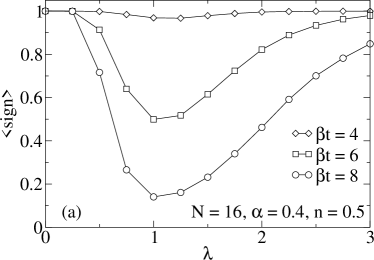
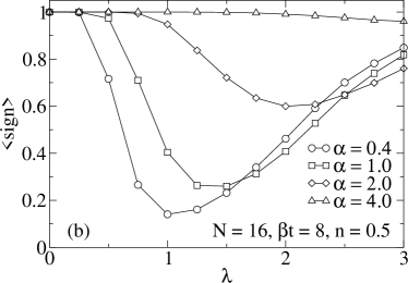
Figure 1: Average sign $\langle\text{sign}\rangle$ in the many-electron case as a function of el-ph coupling $\lambda$ in $\text{D}=1$ (a) for different inverse temperatures $\beta$, and (b) for different values of the adiabaticity ratio $\alpha$. Lines are guides to the eye, and errorbars are smaller than the symbols shown. The data presented in figures 1 and 2 are for $\Delta\tau=0.05$. [Taken from HoNevdLWeLoFe04 .]

Since $w_{\text{b}}$ is strictly positive, we define the average sign as

$$\langle\text{sign}\rangle=\langle w_{\text{f}}\rangle_{\text{b}}/\langle|w_{\text{f}}|\rangle_{\text{b}}\,.$$ (98)

For simplicity, we first show results for $n=0.5$, while the effect of band filling will be discussed later. The choice $n=0.5$ is convenient since we know the chemical potential, and we shall see below that the sign problem is most pronounced for a half-filled band. Moreover, most existing QMC results for the spinless Holstein model are for half filling (see references in HoEvvdL03 ).

Figure 1(a) shows the dependence of $\langle\text{sign}\rangle$ on the el-ph coupling strength. It takes on a minimum near $\lambda=1$ (for $\alpha<1$) that becomes more pronounced with decreasing temperature. At weak coupling (WC) and SC, $\langle\text{sign}\rangle\approx 1$, so that accurate simulations can be carried out. These results are quite similar to the cases of one or two electrons Hohenadler04 .

The dependence on phonon frequency [figure 1(b)] also bears a close resemblance to the polaron problem Hohenadler04 . Whereas $\langle\text{sign}\rangle$ becomes very small for $\alpha\ll 1$, it increases noticeably in the non-adiabatic regime $\alpha>1$, permitting efficient and accurate simulations.

As illustrated in figure 2(a), the average sign depends strongly on the band filling $n$. While it is close to one in the vicinity of $n=0$ or $n=1$ (equivalent to one or two electrons), a significant reduction is visible near half filling $n=0.5$. The minimum occurs at $n=0.5$, and the results display particle-hole symmetry as expected. Here we have chosen $\beta t=8$, $\alpha=0.4$ and $\lambda=1$, for which the sign problem is most noticeable according to figure 1.

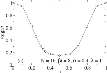
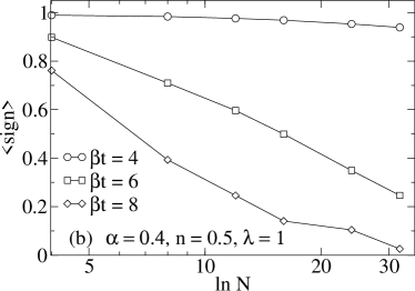
Figure 2: Average sign in the many-electron case as a function of (a) band filling $n$, and (b) system size $N$.

In figure 2(b), we report the average sign as a function of system size, again for $n=0.5$. The dependence is strikingly different from the one-electron case. While in the latter $\langle\text{sign}\rangle\rightarrow 1$ as $N\rightarrow\infty$ HoEvvdL03 ; Hohenadler04 , here the average sign decreases nearly exponentially with increasing system size, a behaviour well-known from QMC simulations of Hubbard models wvl1992 . Obviously, this limits the applicability of our method. However, we shall see below that we can nevertheless obtain accurate results at low temperatures, small phonon frequencies, and over a large range of the el-ph coupling strength. Moreover, we would like to point out that for such parameters, other methods suffer strongly from autocorrelations, rendering simulations extremely difficult.

The dependence of the sign problem on the dimension of the system is again similar to the single-electron case Hohenadler04 . The minimum at intermediate $\lambda$ becomes more pronounced for the same parameters $N$, $\alpha$, $\beta t$ and $\lambda$ as one increases the dimension of the cluster.

To conclude with, we would like to point out that, in principle, the sign problem can be compensated by performing sufficiently long QMC runs, but we have to keep in mind that the statistical errors increase proportional to $\langle\text{sign}\rangle^{-2}$ wvl1992 , setting a practical limit to the accuracy.

5.6 Comparison with other approaches

The QMC method presented above seems to be most advantageous—as compared to other approaches—in the case of the spinless Holstein model with many electrons. For the latter, other methods are severely restricted by autocorrelations, rendering accurate simulations in the physically important adiabatic, IC regime virtually impossible even at moderately low temperatures. In contrast, the present method enables us to study the single-particle spectrum on rather large clusters and for a wide range of model parameters and band filling (see section 6.3). Unfortunately, the generalization to the spinful Hubbard-Holstein model suffers severely from the sign problem.

For the polaron and the bipolaron problem, our method requires more computer time than other QMC algorithms dRLa82 ; deRaLa86 ; Ko98 ; Mac04 . However, we are able to consider practically all parameter regimes on reasonably large clusters in one (polaron and bipolaron problem) and two dimensions (polaron problem).

Finally, a discussion of the scaling of computer time with the system parameters can be found in HoEvvdL03 ; HoEvvdL05 ; HovdL05 .

6 Selected results

We now come to a selection of results obtained with the methods discussed so far, most of which have been published before HoEvvdL03 ; HoEvvdL05 ; HovdL05 ; HoNevdLWeLoFe04 . Note that errorbars will be suppressed in the figures if smaller than the symbolsize. Moreover, lines connecting data points are guides to the eye only.

6.1 Small-polaron cross-over

The Holstein model with a single electron (for a review see FeAlHoWe06 ) exhibits a cross-over from a large polaron ($\text{D}=1$) or a quasi-free electron ($\text{D}>1$) to a small polaron with increasing el-ph coupling strength.

Quantum Monte Carlo

To investigate the small-polaron cross-over, following previous work dRLa82 ; dRLa83 ; Ko97 ; WeRoFe96 ; JeWh98 ; dMeRa97 ; RoBrLi99 ; RoBrLi99III ; KuTrBo02 , we calculate the electronic kinetic energy $E_{\text{kin}}$ given by equation (75). As we shall compare results for different dimensions, we define the normalized quantity

$$\overline{E}_{\text{kin}}=E_{\text{kin}}/(-2t\mathrm{D})$$ (99)

with $\overline{E}_{\text{kin}}=1$ for $T=0$ and $\lambda=0$.

The inverse temperature will be fixed to $\beta t=10$, low enough to identify the cross-over. Calculations at even lower temperatures can easily be done for $\alpha>1$, but $\alpha<1$ requires very large numbers of measurements to ensure satisfactorily small statistical errors. System sizes were 32 sites in 1D, a $12\times 12$ cluster in 2D, and a $6\times 6\times 6$ lattice in 3D. In contrast to $\text{D}=1$, 2, where results are well converged with respect to system size, non-negligible finite-size effects (maximal relative changes of up to 20 % between $N=5$ and $N=6$ for $\alpha\ll 1$; much smaller changes otherwise) are observed in three dimensions. Moreover, for small $N$, effects due to thermal population of states with non-zero momentum $\boldsymbol{k}$—absent in ground-state calculations—are visible, as discussed below. Nevertheless, the main characteristics are well visible already for $N=6$. For a detailed study of finite-size and finite-temperature effects see Hohenadler04 .

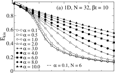
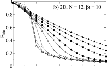
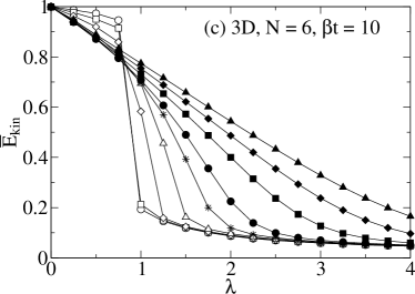
Figure 3: Normalized kinetic energy $\overline{E}_{\text{kin}}$ [equation (99)] of the Holstein model with one electron from QMC as a function of el-ph coupling $\lambda$ for different adiabaticity ratios $\alpha$ and different dimensions D of the lattice ($N$ denotes the linear cluster size). Here and in subsequent figures, QMC data have been extrapolated to $\Delta\tau=0$ (see section 5.2). [Taken from HoEvvdL05 .]

Figure 3 shows $\overline{E}_{\text{kin}}$ as a function of the el-ph coupling $\lambda$ for different phonon frequencies varying over two orders of magnitude, in one to three dimensions. Generally, the kinetic energy is large at WC, where the ground state consists of a weakly dressed electron ($\text{D}>1$) or a large polaron ($\text{D}=1$). It reduces more or less strongly—depending on $\alpha$—in the SC regime, where a small, heavy polaron exists, defined as an electron surrounded by a lattice distortion essentially localized at the same site. The finite values of $\overline{E}_{\text{kin}}$ even for large $\lambda$ are a result of undirected motion of the electron inside the surrounding phonon cloud. In contrast, the quasiparticle weight is exponentially reduced in the SC regime (see, e.g., KuTrBo02 ), whereas the effective mass becomes exponentially large.

In all dimensions, the phonon frequency has a crucial influence on the behaviour of the kinetic energy. While in the adiabatic regime $\alpha<1$ the small-polaron cross-over is determined by the condition $\lambda=E_{\text{P}}/2t\text{D}>1$, the corresponding criterion for $\alpha>1$ is $g^{2}=E_{\text{P}}/\omega_{0}>1$. The former condition reflects the fact that the loss in kinetic energy of the electron has to be outweighed by a gain in potential energy in order to make small-polaron formation favourable. The latter condition expresses the increasing importance of the lattice energy for $\alpha>1$, since the formation of a “localized” state requires a sizable lattice distortion. As a consequence, for large phonon frequencies, the critical coupling shifts to $\lambda_{\mathrm{c}}>1$, whereas for $\alpha<1$ we have $\lambda_{\mathrm{c}}=1$. Additionally, the decrease of $\overline{E}_{\text{kin}}$ at $\lambda_{\mathrm{c}}$ becomes significantly sharper with decreasing phonon frequency.

Concerning the effect of dimensionality, figure 3 reveals that, for fixed $\alpha$, the small-polaron cross-over becomes more abrupt in higher dimensions, with a very sharp decrease in 3D. Nevertheless, there is no real phase transition Loe88 . Figure 3 also contains results for $N=6$ in one and two dimensions, i.e., for the same linear cluster size as in 3D (dashed lines). Clearly, for such small clusters, the spacing between the discrete allowed momenta $\boldsymbol{k}$ is too large to permit substantial thermal population, so that results are closer to the ground state [e.g., $\overline{E}_{\text{kin}}(\lambda=0)\approx 1$], and exhibit a slightly more pronounced decrease near the critical coupling. However, the sharpening of the latter with increasing dimensionality is still well visible.

Variational approach

To test the validity of the variational approach of section 4 we have calculated the total energy [equation (24)] and the quasiparticle weight [equation (29)] on a cluster with $N=4$ for various values of $\alpha$. A comparison with exact diagonalization results Mars95 is depicted in figure 4. We only consider the regime $\alpha\geq 1$ where the zero-phonon approximation is expected to be justified. The overall agreement is strikingly good. Minor deviations from the exact results increase with decreasing $\alpha$. For the smallest frequency shown, $\alpha=1$, the result of the HLF approximation is also reported. Clearly, the variational method represents a significant improvement over the HLF approximation, underlining the importance of taking into account non-local distortions. Similar conclusions can be drawn for larger system sizes (see figure 3 in HoEvvdL03 ).

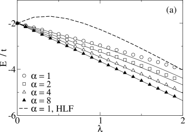
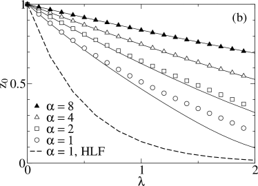
Figure 4: Total energy $E$ (a) and quasiparticle weight $z_{0}$ (b) for $N=4$ as functions of the el-ph coupling $\lambda$ for different values of the adiabaticity ratio $\alpha$. Symbols correspond to variational results and full lines represent exact $T=0$ data obtained with the Lanczos method Mars95 . Dashed lines are results of the HLF approximation. [Taken from HoEvvdL03 .]

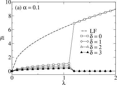
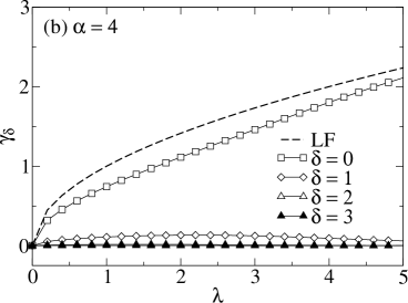
Figure 5: Polaron-size parameter $\gamma_{\delta}$ for $N=16$ as a function of the el-ph coupling $\lambda$ for various distances $\delta$ in the (a) adiabatic and (b) anti-adiabatic regime. Also shown is the LF parameter $\gamma$ [equation (10)]. [Taken from HoEvvdL03 .]

In figure 5 we present results for the variational displacement fields $\gamma_{\delta}$, which provide a measure for the polaron size. For $\alpha=0.1$ we see an abrupt cross-over from a large to a small polaron at $\lambda\approx 1.2$. For smaller $\lambda$, the electron induces lattice distortions at neighboring sites even at a distance of more than three lattice constants. Above $\lambda\approx 1.2$ we have a mobile small polaron extending over a single site only. In contrast, for the anti-adiabatic case $\alpha=4$, the cross-over is much more gradual, and $\gamma_{1}>0$ even for $\lambda\gg 1$. The same behaviour has been found by Marsiglio Marsiglio95 who determined the correlation function $\langle\widehat{n}_{i}\widehat{x}_{i+\delta}\rangle$ by exact diagonalization; within the variational approach $\langle\widehat{n}_{i}\widehat{x}_{i+\delta}\rangle=\gamma_{\delta}$. Although in Marsiglio’s results the cross-over to a small polaron for $\alpha=0.1$ occurs at a smaller value of the coupling $\lambda\approx 1$, the simple variational approach reproduces the main characteristics.

6.2 Bipolaron formation in the extended Holstein-Hubbard model

In contrast to Cooper pairing of electrons with opposite momentum, two electrons may also form a bound state by travelling sufficiently close in real space. Bipolaron formation may be studied in the framework of the 1D extended Holstein-Hubbard model, and a brief review of previous work has been given in HoAivdL04 ; HovdL05 . Here we merely note that depending on the choice of parameters, the ground state of the model may either consist of two polarons, a large bipolaron, an inter-site bipolaron or a small bipolaron (in the singlet case). A summary of the conditions on the model parameters is given in table 1. Whereas existing work is almost exclusively concerned with the singlet case, here we shall also consider two electrons of the same spin. Triplet bipolarons are expected to play a role, e.g., in the ferromagnetic state of the manganites AlBr99 ; AlBr99_2 ; David_AiP . Furthermore, we are not aware of any previous work for $V>0$.

Table 1: Conditions for the existence of different singlet bipolaron states in the one-dimensional Holstein-Hubbard model HovdL05 .

$U=0$				$U>0$
Large bipolaron			Small bipolaron	Two	Inter-site	Small
				polarons	bipolaron	bipolaron
$\lambda<0.5$			$\lambda>0.5$	$U>2E_{\text{P}}$ (WC)	$U<2E_{\text{P}}$ (WC)
or			and			$U\ll 2E_{\text{P}}$
$g<0.5$			$g>0.5$	$U>4E_{\text{P}}$ (SC)	$U<4E_{\text{P}}$ (SC)

Quantum Monte Carlo

Owing to the increased numerical effort compared to the one-electron case, we shall only present results for $N\leq 12$ in one dimension. However, finite-size effects are small even for the most critical parameters HovdL05 .

We define the effective kinetic energy of the two electrons as

$$\overline{E}_{\text{kin}}=E_{\text{kin}}/(-4t)\,.$$ (100)

In figure 6(a) we depict $\overline{E}_{\text{kin}}$ as a function of the el-ph coupling for different values of $\alpha$ and $U/t$, at $\beta t=10$, i.e., much closer to the ground state than in some previous work deRaLa86 .

Figure 6(a) reveals a strong decrease of $\overline{E}_{\text{kin}}$ near $\lambda=0.5$ for $\alpha=0.4$ and $U/t=0$. With increasing $\alpha$, the cross-over becomes less pronounced, and shifts to larger values of $\lambda$. For the same value of $\alpha$, the cross-over to a small bipolaron is sharper than the small-polaron cross-over [cf figure 3(a)]. For finite on-site repulsion $U/t=4$, $\overline{E}_{\text{kin}}$ remains fairly large up to $\lambda\approx 1$ (for $\alpha=0.4$), in agreement with the SC result $\lambda_{\text{c}}=1$ for $U/t=4$ (see discussion in HoAivdL04 ). At even stronger coupling, the Hubbard repulsion is overcome, and a small bipolaron is formed. Again, the critical coupling increases with phonon frequency. Finally, the kinetic energy in the triplet case (corresponding to $U/t=\infty$) is comparable to the results for $U/t=4$ up to $\lambda\approx 1$, but significantly larger in the SC regime since on-site bipolaron formation is not possible.

The influence of nearest-neighour repulsion $V$ is revealed in figure 6(b), again for $U/t=4$. For all values of $\alpha$ shown, the cross-over sharpens noticeably for $V>0$. The reason is that $V>0$ suppresses the (more mobile) inter-site bipolaron state, leading to a direct cross-over from a large to a small bipolaron.

The nature of the bipolaron state is revealed by the correlation function $\rho(\delta)$ [equation (81)], which gives the probability for the two electrons to be separated by a distance $\delta\geq 0$, and provides a measure of the bipolaron size. The phonon frequency determines the degree of retardation of the el-ph interaction, and thereby limits the distance between the two electrons in a bound state. In the sequel, we shall focus on the most interesting case of small phonon frequencies, which has often been avoided in previous work for reasons outlined in section 5.

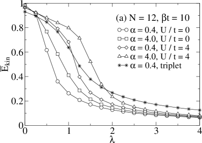
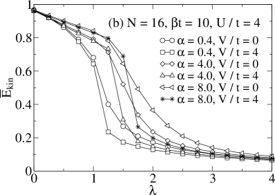
Figure 6: Normalized kinetic energy $\overline{E}_{\text{kin}}$ [equation (100)] from QMC as a function of the el-ph coupling $\lambda$ for different values of the adiabaticity ratio $\alpha$, the on-site repulsion $U$ and the nearest-neighbour repulsion $V$. [(a) taken from HovdL05 .]

Starting with $U\ll E_{\text{P}}$, a cross-over from a small to an inter-site bipolaron to two weakly bound polarons takes place upon increasing the Hubbard interaction BoKaTr00 . Since the latter competes with the retarded el-ph interaction, the phonon frequency is expected to be an important parameter. In figure 7, we show the kinetic energy and the correlation function $\rho(\delta)$ as a function of $U/t$ for IC $\lambda=1$. Starting from a small bipolaron for $U/t=0$, the kinetic energy increases with increasing Hubbard repulsion, equivalent to a reduction of the effective bipolaron mass BoKaTr00 ; ElShBoKuTr03 . Although the cross-over is slightly washed out by the finite temperature in our simulations, there is a well-conceivable increase in $\overline{E}_{\text{kin}}$ up to $U/t\approx 4$, above which the kinetic energy begins to decrease slowly. The increase of $\overline{E}_{\text{kin}}$ originates from the breakup of the small bipolaron, as indicated by the decrease of $\rho(0)$ in figure 7(b). Close to $U/t=4$, the curves for $\rho(0)$ and $\rho(1)$ cross, and it becomes more favourable for the two electrons to reside on neighboring sites. The inter-site bipolaron only exists below a critical Hubbard repulsion $U_{\text{c}}$. The latter is given by $U_{\text{c}}=2E_{\text{P}}$ (i.e., here $U_{\text{c}}/t=4$) at weak el-ph coupling, and by $U_{\text{c}}=4E_{\text{P}}$ at SC. For an intermediate value $\lambda=1$ as in figure 7, the cross-over from the inter-site state to two weakly bound polarons is expected to occur somewhere in between, but is difficult to locate exactly from the QMC results.

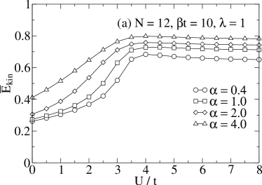
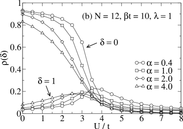
Figure 7: (a) Normalized kinetic energy $\overline{E}_{\text{kin}}$ and (b) correlation functions $\rho(0)$, $\rho(1)$ from QMC as a function of the Hubbard repulsion $U/t$ for different values of the adiabaticity ratio $\alpha$. [Taken from HovdL05 .]

Figure 7 further illustrates that the cross-over becomes steeper with decreasing phonon frequency. In the adiabatic limit $\alpha=0$, it has been shown to be a first-order phase transition PrAu99 , whereas for $\alpha>0$ retardation effects suppress any non-analytic behaviour. At the same $U/t$, $\overline{E}_{\text{kin}}$ increases with $\alpha$ since for a fixed $\lambda$, the bipolaron becomes more weakly bound. For the same reason, the cross-over to an inter-site bipolaron—showing up in figure 7 as a crossing of $\rho(0)$ and $\rho(1)$—shifts to smaller values of $U/t$.

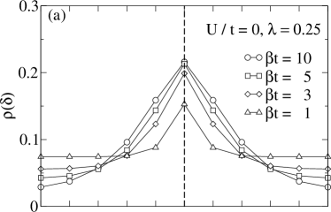
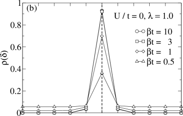
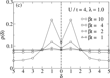
Figure 8: Correlation function $\rho(\delta)$ from QMC as a function of $\delta$ for different inverse temperatures $\beta$, $N=12$ and $\alpha=0.4$. [Taken from HovdL05 .]

Let us now consider the effect of temperature on $\rho(\delta)$. To this end, we plot in figures 8(a) – (c) $\rho(\delta)$ at different temperatures, for parameters corresponding to the three regimes of a large, small and inter-site bipolaron, respectively.

For the parameters in figure 8(a) ($U/t=0$, $\lambda=0.25$), the two electrons are most likely to occupy the same site, but the bipolaron extends over a distance of several lattice constants. Clearly, in this regime, the cluster size $N=12$ used here is not completely satisfactory, but still provides a fairly accurate description as can be deduced from calculations for $N=14$ (not shown). Nevertheless, on such a small cluster, no clear distinction between an extended bipolaron and two weakly bound polarons can be made. As the temperature increases from $\beta t=10$ to $\beta t=1$, the probability distribution broadens noticeably, i.e., it becomes more likely for the two electrons to be further apart. In particular, for the highest temperature shown, $\rho(0)$ has reduced by about 30 % compared to $\beta t=10$.

A different behaviour is observed for the small bipolaron, which exist at stronger el-ph coupling $\lambda=1$. Figure 8(b) reveals that $\rho(\delta)$ peaks strongly at $\delta=0$, but is very small for $\delta>0$ at low temperatures. Increasing temperature, $\rho(\delta)$ remains virtually unchanged up to $\beta t=3$. Only at very high temperatures there occurs a noticeable transfer of probability from $\delta=0$ to $\delta>0$. At the highest temperature shown, $\beta t=0.5$, the two electrons have a non-negligible probability for traveling a finite distance $\delta>0$ apart, although most of the probability is still contained in the peak located at $\delta=0$.

Finally, we consider in figure 8(c) the inter-site bipolaron, taking $U/t=4$ and $\lambda=1$ (cf figure 2 in HovdL05 ). At low temperatures, $\rho(\delta)$ takes on a maximum for $\delta=1$. For smaller values of $\beta t$, the latter diminishes, until at $\beta t=1$, the distribution is completely flat, so that all $\delta$ are equally likely.

The different sensitivity of the bipolaron states to changes in temperature found above can be explained by their different binding energies. The latter is given by $\Delta E_{0}=E_{0}^{(2)}-2E_{0}^{(1)}$, where $E_{0}^{(1)}$ and $E_{0}^{(2)}$ denote the ground-state energy of the model with one and two electrons, respectively.

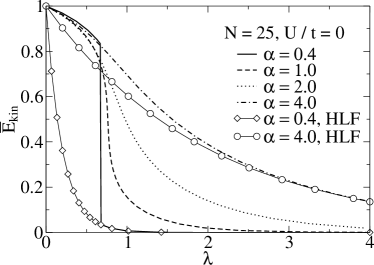
Figure 9: Variational results for the normalized kinetic energy $\overline{E}_{\text{kin}}$ as a function of the el-ph coupling $\lambda$, and for different adiabaticity ratios $\alpha$. Also shown are results of the HLF approximation. [Taken from HovdL05 .]

Generally, the thermal dissociation is expected to occur at a temperature such that the thermal energy $k_{\text{B}}T=(\beta T)^{-1}$ becomes comparable to $\Delta E_{0}$, in accordance with our numerical data. The large and the inter-site bipolaron are relatively weakly bound as a result of the rather small effective interaction $U_{\text{eff}}\approx U-2E_{\text{P}}$ HoAivdL04 . The binding energies are $\Delta E_{0}\approx-(0.32\pm 0.08)t$ and $-(0.28\pm 0.08)t$, respectively, so that we expect a critical inverse temperature $\beta t\approx 2.5$ – 5, in agreement with figures 8(a) and (c). In contrast, the small bipolaron in figure 8(b) has a significantly larger binding energy $\Delta E\approx-(3.43\pm 0.09)t$, and therefore remains stable up to $\beta t\approx 0.3$. Thermal dissociation of bipolarons occurs at even lower temperatures for $V>0$, especially in the triplet case, owing to the reduced binding energy.

Variational approach

Whereas the QMC approach is limited to finite temperatures and relatively small clusters, the variational method of section 4 yields ground-state results on much larger systems. To scrutinize the quality of the variational method, we compare the ground-state energy for $U/t=0$ to the most accurate approach currently available in one dimension, namely the variational diagonalization BoKaTr00 . We find a good agreement over the whole range of $\lambda$. As expected from the nature of the approximation, slight deviations occur for $\alpha\lesssim 1$, similar to the one-electron case.

Despite the success in calculating the total energy—being the quantity that is optimized—one has to be careful not to overestimate the validity of any variational method. To reveal the shortcomings of the current approach, we show in figure 9 the normalized kinetic energy $\overline{E}_{\text{kin}}=t_{\text{eff}}$ [see equations (31) and (100)] as a function of el-ph coupling, and for different $\alpha$. We have chosen $N=25$ to ensure negligible finite-size effects. In principle, figure 9 displays a behaviour similar to the QMC data in figure 6(a). There is a jump-like decrease of $\overline{E}_{\text{kin}}$ near $\lambda=0.5$ for $\alpha=0.4$, which becomes washed out and moves to larger $\lambda$ with increasing phonon frequency. For $\alpha=0.4$, the cross-over in the variational results is much too steep, regardless of the fact that the latter are for $T=0$, a common defect of variational methods. Moreover, for $\alpha=0.4$ – 2, the variational kinetic energy is too small above the bipolaron cross-over compared to the QMC data, whereas for $\alpha=4$, the decay of $\overline{E}_{\text{kin}}$ with increasing $\lambda$ is too slow.

The reason for the failure is the absence of retardation effects, which play a dominant role in the formation of bipolaron states. The increased importance of the phonon dynamics—not included in the variational method—for the two-electron problem leads to a less good agreement with exact results than in the one-electron case. In particular, our variational results overestimate the position of the cross-over (figure 9) compared to the value $\lambda_{\text{c}}=0.5$ expected in the adiabatic regime. Nevertheless, the method represents a significant improvement over the simple HLF approximation, due to the variational determination of the parameters $\gamma_{ij}$. This is illustrated in figure 9, where we also show the HLF result $\overline{E}_{\text{kin}}=\mathrm{e}^{-g^{2}}$ for $\alpha=0.4$ and 4.0. In contrast to the variational approach, the HLF approximation yields an exponentially decreasing kinetic energy for all values of the phonon frequency. Whereas such behaviour actually occurs in the anti-adiabatic limit $\alpha\to\infty$, the situation is different for small $\alpha$ [see figures 6(a) and 9]. The variational method presented here accounts qualitatively for the influence of the phonon frequency on bipolaron formation.

Figure 10: One-electron spectral function $A(k,\omega-\mu)$ from QMC for different band fillings $n$, $N=32$, $\beta t=8$, $\alpha=0.4$, and $\lambda=0.1$. Here and in subsequent figures $\Delta\tau=0.1$. [Taken from HoNevdLWeLoFe04 .]

6.3 Many-polaron problem

We review recent results on the carrier-density dependence of photoemission spectra of many-polaron systems in the framework of the spinless Holstein model (63) in one dimension. We shall see that the sensitivity to changes in $n$ strongly depends on the phonon frequency and el-ph coupling strength, with the most interesting physics being observed in the adiabatic, IC regime often realized experimentally. This regime is characterized by the existence of large polarons at low carrier density. At larger densities, a substantial overlap of the single-particle wavefunctions occurs, leading to a dissociation of the individual polarons and finally to a restructuring of the whole many-particle ground state. Note that the many-polaron problem has since been studied also by means of other methods LoHoFe06 ; HoWeAlFe05 ; WeBiHoScFe05 , confirming the original findings of HoNevdLWeLoFe04 .

Weak coupling

For WC $\lambda=0.1$, the sign problem is not severe (section 5.5) so that simulations can easily be performed for large lattices with $N=32$, making the dispersion of quasiparticle features well visible.

Figure 10 shows the evolution of the one-electron spectral function $A(k,\omega-\mu)$ with increasing electron density $n$. At first sight, we see that the spectra bear a close resemblance to the free-electron case, i.e., there is a strongly dispersive band running from $-2t$ to $2t$ which can be attributed to weakly dressed electrons. As expected, the height (width) of the peaks increases (decreases) significantly in the vicinity of the Fermi momentum $k_{\text{F}}$, determined by the crossing of the band with the chemical potential. However, in contrast to the case of a rigid tight-binding band, we shall see below (figure 11) that a significant redistribution of spectral weight occurs with increasing $n$.

Figure 11: One-electron density of states $N(\omega-\mu)$ from QMC for different band fillings $n$, $N=32$, $\beta t=8$, $\alpha=0.4$ and $\lambda=0.1$. [Taken from HoNevdLWeLoFe04 .]

We would like to point out that the apparent absence of any phonon signatures in figure 10 is not a defect of the maximum entropy method, but results from the large scale of the $z$-axis chosen. As a consequence, the peaks running close to the bare band dominate the spectra and suppress any small phonon peaks present. At higher resolution, for all densities $n=0.1$ – 0.4, we observe the band flattening Stephan ; WeFe97 ; HoAivdL03 at large wavevectors which originates from the intersection of the approximately free-electron dispersion with the bare phonon energy at $\omega-\mu=\omega_{0}$.

To complete our discussion of the WC regime, we show in figure 11 the one-electron density of states (DOS) $N(\omega-\mu)$ given by equation (94). Clearly, for small $n$, there is a peak with large spectral weight at the Fermi level. In contrast, for large $n$, the tendency toward formation of a Peierls– (band–) insulating state at $n=0.5$ suppresses the DOS at the Fermi level, although we are well below the critical value of $\lambda$ at which the cross-over to the insulating state takes place at $T=0$ BuMKHa98 ; HoWeBiAlFe06 . The additional small features separated from $\mu$ by the bare phonon energy $\omega_{0}$ will be discussed below.

Strong coupling

Figure 12: One-electron spectral function $A(k,\omega-\mu)$ from QMC for different band fillings $n$, $N=32$, $\beta t=8$, $\alpha=0.4$, and $\lambda=2$. [Taken from HoNevdLWeLoFe04 .]

We now turn to the SC limit taking $\lambda=2$. At low density $n=0.1$ [figure 12(a)], we expect the well-known, almost flat polaron band having exponentially reduced spectral weight (given by $e^{-g^{2}}$ in the single-electron, SC limit) which, nevertheless, can give rise to coherent transport at $T=0$. As discussed in HoNevdLWeLoFe04 , such weak signatures are difficult to determine accurately using the maximum entropy method. Generally, it is known that the reliability of dynamic properties obtained by means of the maximum entropy method crucially depends on the size of statistical errors and the general structure of the spectra. A detailed discussion of this point has been given in HoNevdLWeLoFe04 .

Besides, the spectrum consists of two incoherent features located above and below the chemical potential, which reflect the phonon-mediated transitions to high-energy electron states. Here, the maximum of the photoemission spectra ($\omega-\mu>0$) follows a tight-binding cosine dispersion. The incoherent part of the spectra is broadened according to the phonon distribution.

For all band fillings, the chemical potential is expected to be located in a narrow polaron band with little spectral weight. There exists a finite gap to the photoemission (inverse photoemission) parts of the spectrum, so that the system typifies as a polaronic metal. We shall see below that a completely different behaviour is observed at IC. Notice that the incoherent inverse photoemission (photoemission) signatures are more pronounced at small (large) wavevectors.

Finally, for $n=0.4$ [figure 12(d)], the incoherent features lie rather close to the Fermi level, thus being accessible by low-energy excitations. Now, the photoemission spectrum for $k<\pi/2$ is almost symmetric to the inverse photoemission spectrum for $k>\pi/2$ and already reveals the gapped structure which occurs at $n=0.5$ due to charge-density-wave formation accompanied by a Peierls distortion HoWeBiAlFe06 .

As in the WC case discussed above, the properties of the system also manifest itself in the DOS, shown in figure 13. Owing to the strong el-ph interaction, the spectral weight at the chemical potential is exponentially small for all fillings $n$. At half filling, the DOS exhibits particle-hole symmetry, and the system can be described as a Peierls insulator, consisting of a polaronic superlattice. In contrast to the WC case, the ground state is characterized as a polaronic insulator rather than as a band insulator.

Figure 13: One-electron density of states $N(\omega-\mu)$ from QMC for different band fillings $n$ and cluster sizes $N$, $\beta t=8$, $\alpha=0.4$ and $\lambda=2$. [Taken from HoNevdLWeLoFe04 .]

Intermediate coupling

As discussed in the introduction, a cross-over from a polaronic state to a system with weakly dressed electrons can be expected in the IC regime. Here we choose $\lambda=1$, which corresponds to the critical value for the small-polaron cross-over in the one-electron problem [cf figure 3(a)]. Owing to the sign problem, which is particularly noticeable for $\lambda=1$ (see figure 1), we have to decrease the system size as we increase the electron density $n$.

Figure 14: One-electron spectral function $A(k,\omega-\mu)$ from QMC for different band fillings $n$ and cluster sizes $N$, $\beta t=8$, $\alpha=0.4$, and $\lambda=1$. [Taken from HoNevdLWeLoFe04 .]

We shall see that the cross-over is rather difficult to detect from the QMC results only. However, the data presented here are perfectly consistent with more recent studies employing other methods such as exact diagonalization HoNevdLWeLoFe04 , cluster perturbation theory HoWeAlFe05 or self-energy calculations LoHoFe06 .

Figure 14 shows the spectral function for $\lambda=1$ and increasing band filling. Owing to the overlap of large polarons in the IC regime, we start with a very low density $n=0.05$ [figure 14(a)]. Compared to the behaviour for $\lambda=2$ [figure 12(a)], we notice that the polaron band now lies much closer to the incoherent features, and that there is a mixing of these two parts of the spectrum at small values of $k$. Nevertheless, the almost flat polaron band is well visible for large $k$.

With increasing density, the polaron band merges with the incoherent peaks at higher energies, signaling the above-anticipated density-driven cross-over from a polaronic to a (diffusive) metallic state, with the broad main band crossing the Fermi level.

Further information about the density dependence can be obtained from the one-electron DOS. The latter is presented in figure 15 for different fillings $n=0.05$ – 0.5. As in figure 14, the cluster size is reduced with increasing $n$ in order to cope with the sign problem. To illustrate the rather small influence of finite-size effects, figure 15 also contains results for $N=10$.

For low density $n=0.05$, the DOS in figure 15 lies in between the results for WC and SC discussed above. Although the spectral weight at the chemical potential is strongly reduced compared to $\lambda=0.1$, $N(0)$ is still significantly larger than for $\lambda=2$.

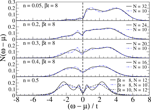
Figure 15: One-electron density of states $N(\omega-\mu)$ from QMC for different band fillings $n$, cluster sizes $N$ and inverse temperatures $\beta$. Here $\alpha=0.4$ and $\lambda=1$. [Taken from HoNevdLWeLoFe04 .]

When the density is increased to $n=0.2$, the DOS at the chemical potential increases, as a result of the dissociation of polarons. Increasing $n$ further, a pseudogap begins to form at $\mu$, which is a precursor of the charge-density-wave gap at half filling and zero temperature.

In the case of half filling $n=0.5$, the DOS has become symmetric with respect to $\mu$. There are broad features located either side of the chemical potential, which take on maxima close to $\omega-\mu=\pm E_{\text{P}}$. However, apart from the SC case, where the single-polaron binding energy is still a relevant energy scale, the position of these peaks is rather determined by the energy of the upper and lower bands, split by the formation of a Peierls state. The gap of size $\sim\lambda$ expected for the insulating charge-ordered state at $T=0$ is partially filled in due to the finite temperature considered here.

Furthermore, we find additional, much smaller features roughly separated from $\mu$ by the bare phonon frequency $\omega_{0}$, whose height decreases with decreasing temperature, as revealed by the results for $\beta t=10$ (figure 15). These peaks—not present at $T=0$ SyHuBeWeFe04 ; HoWeBiAlFe06 —arise from thermally activated transitions to states with additional phonons excited, and are also visible in figures 11 and 13. While for WC ($\lambda=0.1$, figure 11), the maximum of these features is almost exactly located at $|\omega-\mu|=\omega_{0}$, it moves to $|\omega-\mu|\approx 1.25\omega_{0}$ for IC ($\lambda=1$, figure 15), and finally to $|\omega-\mu|\approx 2.5\omega_{0}$ for SC ($\lambda=2$, figure 13). Although the exact positions of the peaks are subject to uncertainties due to the maximum entropy method, this evolution reflects the shift of the maximum in the phonon distribution function with increasing coupling. The maximum entropy method yields an envelope of the multiple peaks separated by $\omega_{0}$.

Anti-adiabatic regime

The comparison of the spectral functions for $n=0.1$ and $n=0.3$ in figure 10 of HoNevdLWeLoFe04 reveals that there is no density-driven cross-over of the system as observed in the adiabatic case even for the critical value $g^{2}=1$. In particular, owing to the large phonon energy, there are no low-energy excitations close to the polaron band, so that the latter remains well separated from the incoherent features even for $n=0.3$. Furthermore, the spectral weight of the polaron band also remains almost unchanged as we increase the density from $n=0.1$ to $n=0.3$. Consequently, almost independent small polarons are formed also at finite electron densities, in accordance with previous findings for small systems CaGrSt99 .

7 Summary

We have reviewed quantum Monte Carlo and variational approaches to Holstein models based on Lang-Firsov transformations of the Hamiltonian. The methods have been applied to investigate single polarons and bipolarons, respectively, as well as a many-polaron system.

The variational methods include displacements of the lattice at all lattice sites, which enables them to quite accurately describe large polaron or bipolaron states.

Using the transformed Hamiltonian, we have shown that quantum Monte Carlo simulation can be based on exact sampling without autocorrelations, which proves to be an enormous advantage for small phonon frequencies or low temperatures. Indeed, we have used a grand-canonical algorithm to obtain dynamical properties of many-polaron systems in all interesting parameter regimes. Such simulations are currently not possible with other Monte Carlo methods.

References

- (1) I. G. Lang and Y. A. Firsov, Zh. Eksp. Teor. Fiz. 43, 1843 (1962), [Sov. Phys. JETP 16, 1301 (1962)].
- (2) T. Holstein, Ann. Phys. (N.Y.) 8, 325; 8, 343 (1959).
- (3) G. D. Mahan, Many-Particle Physics, 2nd ed. (Plenum Press, New York, 1990).
- (4) E. V. L. de Mello and J. Ranninger, Phys. Rev. B 55, 14 872 (1997).
- (5) J. M. Robin, Phys. Rev. B 56, 13 634 (1997).
- (6) H. Fehske, J. Loos, and G. Wellein, Phys. Rev. B 61, 8016 (2000).
- (7) M. Hohenadler, H. G. Evertz, and W. von der Linden, Phys. Rev. B 69, 024301 (2004).
- (8) C. Zhang, E. Jeckelmann, and S. R. White, Phys. Rev. B 60, 14 092 (1999).
- (9) M. Hohenadler and W. von der Linden, Phys. Rev. B 71, 184309 (2005).
- (10) M. Hohenadler, H. G. Evertz, and W. von der Linden, phys. stat. sol. (b) 242, 1406 (2005).
- (11) M. Hohenadler et al., Phys. Rev. B 71, 245111 (2005).
- (12) W. von der Linden, Phys. Rep. 220, 53 (1992).
- (13) E. Y. Loh and J. E. Gubernatis, in Electronic Phase Transitions, edited by W. Hanke and Y. V. Kopaev (Elsevier Science Publishers, North-Holland, Amsterdam, 1992), Chap. 4.
- (14) R. Blankenbecler, D. J. Scalapino, and R. L. Sugar, Phys. Rev. D 24, 2278 (1981).
- (15) J. E. Hirsch, Phys. Rev. B 31, 4403 (1985).
- (16) G. Wellein, H. Röder, and H. Fehske, Phys. Rev. B 53, 9666 (1996).
- (17) M. Brunner, S. Capponi, F. F. Assaad, and A. Muramatsu, Phys. Rev. B 63, R180511 (2001).
- (18) E. Jeckelmann and S. R. White, Phys. Rev. B 57, 6376 (1998).
- (19) A. H. Romero, D. W. Brown, and K. Lindenberg, Phys. Rev. B 60, 14080 (1999).
- (20) L. C. Ku, S. A. Trugman, and J. Bonča, Phys. Rev. B 65, 174306 (2002).
- (21) M. Jarrell and J. E. Gubernatis, Phys. Rep. 269, 133 (1996).
- (22) A. C. Davison and D. V. Hinkley, Bootstrap Methods and their Application (Cambridge University Press, Cambridge, UK, 1997).
- (23) W. H. Press, Numerical Recipes in Fortran 77, http://www.numrec.com.
- (24) M. Hohenadler, Ph.D. thesis, TU Graz, 2004.
- (25) H. De Raedt and A. Lagendijk, Phys. Rev. Lett. 49, 1522 (1982).
- (26) H. De Raedt and A. Lagendijk, Z. Phys. B: Condens. Matter 65, 43 (1986).
- (27) P. E. Kornilovitch, Phys. Rev. Lett. 81, 5382 (1998).
- (28) A. Macridin, G. A. Sawatzky, and M. Jarrell, Phys. Rev. B 69, 245111 (2004).
- (29) H. Fehske, A. Alvermann, M. Hohenadler, and G. Wellein, in Polarons in Bulk Materials and Systems with Reduced Dimensionality, Proc. Int. School of Physics “Enrico Fermi”, Course CLXI, edited by G. Iadonisi, J. Ranninger, and G. De Filippis (IOS Press, Amsterdam, Oxford, Tokio, Washington DC, 2006), pp. 285–296.
- (30) H. De Raedt and A. Lagendijk, Phys. Rev. B 27, 6097 (1983).
- (31) P. E. Kornilovitch, J. Phys.: Condens. Matter 9, 10675 (1997).
- (32) A. H. Romero, D. W. Brown, and K. Lindenberg, Phys. Lett. A 254, 287 (1999).
- (33) H. Lowen, Phys. Rev. B 37, 8661 (1988).
- (34) F. Marsiglio, in Recent Progress in Many-Body Theories, edited by E. Schachinger, H. Mitter, and H. Sormann (Plenum Press, New York, 1995), Vol. 4.
- (35) F. Marsiglio, Physica C 244, 21 (1995).
- (36) M. Hohenadler, M. Aichhorn, and W. von der Linden, Phys. Rev. B 71, 014302 (2005).
- (37) A. S. Alexandrov and A. M. Bratkovsky, Phys. Rev. Lett. 82, 141 (1999).
- (38) A. S. Alexandrov and A. M. Bratkovsky, J. Phys.: Condens. Matter 11, L531 (1999).
- (39) D. M. Edwards, Adv. Phys. 51, 1259 (2002).
- (40) J. Bonča, T. Katrašnik, and S. A. Trugman, Phys. Rev. Lett. 84, 3153 (2000).
- (41) S. El Shawish, J. Bonča, L. C. Ku, and S. A. Trugman, Phys. Rev. B 67, 014301 (2003).
- (42) L. Proville and S. Aubry, Eur. Phys. J. B 11, 41 (1999).
- (43) J. Loos, M. Hohenadler, and H. Fehske, J. Phys.: Condens. Matter 18, 2453 (2006).
- (44) M. Hohenadler, G. Wellein, A. Alvermann, and H. Fehske, Physica B 378-380, 64 (2006).
- (45) G. Wellein et al., Physica B 378-380, 281 (2006).
- (46) W. Stephan, Phys. Rev. B 54, 8981 (1996).
- (47) G. Wellein and H. Fehske, Phys. Rev. B 56, 4513 (1997).
- (48) M. Hohenadler, M. Aichhorn, and W. von der Linden, Phys. Rev. B 68, 184304 (2003).
- (49) R. J. Bursill, R. H. McKenzie, and C. J. Hamer, Phys. Rev. Lett. 80, 5607 (1998).
- (50) M. Hohenadler et al., Phys. Rev. B 73, 245120 (2006).
- (51) S. Sykora et al., Phys. Rev. B 71, 045112 (2005).
- (52) M. Capone, M. Grilli, and W. Stephan, Eur. Phys. J. B 11, 551 (1999).