Density of states of a two dimensional XY model from Wang-Landau algorithm

Abstract

Using Wang-landau algorithm combined with analytic method, the density of states of two dimensional XY model on square lattices of sizes $16\times 16$, $24\times 24$ and $32\times 32$ is accurately calculated. Thermodynamic quantities, such as internal energy, free energy, entropy and specific heat are obtained from the resulted density of states by numerical integration. From the entropy curve symptoms of phase transition is observed. A general method of calculation of the density of states of continuous models by simulation combined with analytical method is proposed.

I INTRODUCTION

The XY model has been widely used in description of many physical systems and in the studies of phase transitions and other related problems. The two dimensional XY model is especially interested in the studies of the KT transition. The model has been extensively studied in the past decades with many different methods, while the density of states(DOS) is yet not determined because of the complexity of the model. R. Toral and his group computed the DOS of one dimensional XY model and got some scaling resultsRRA2002PA ; R2004JSP . However, the two dimensional XY model is more interesting and valuable. It is famous for its quasi-long range order, vortex pairs and KT phase transition JV1979PRB . It will be helpful for people to understand the nature of the model and study in more details of the KT phase transition if the DOS of the two dimensional XY model is calculated.

The model can be described by the Hamiltonian:

$$H=-J{\sum_{<ij>}}{\vec{S}_{i}}{\cdot}{\vec{S}_{j}}$$ (1)

where $J$ is the coupling constant, and ${\vec{S}}$ is a unit vector(the spin) in a plane. Here $i$ or $j$ is the lattice site on a plane, and the summation is over all nearest neighbor pairs. Different from the Ising model, the XY model is a continuous model in which the energy changes continuously. Thus the total number of states of the whole system is infinite, this property gives rise to the difficulties in determining the DOS near the highest and lowest energy level, as we will explain in detail later.

Recently many kinds of simulation algorithms used in the calculation of the DOS have been proposed, in this study we use Wang-Landau algorithm to calculate the DOS of a two dimensional XY modelWL2001PRL ; WL2001PRE . The fast convergence, stability and easy to implement of the method makes it the first choice in a DOS calculation, however, it has some shortcomings in the accuracy of calculation as pointed out by many researchersCR2001PRE . In the case of the two dimensional XY model and other continuous models alike, the algorithm usually fails to give good results of DOS close the the boundaries of the spectrum. Fortunately, on the spectrum boundaries, there are usually analytical results of the DOS available or may be obtained in less effort. By combining the analytical results close to spectrum boundaries with simulation, better results of the DOS can be obtained. In the following we show this process using the two dimensional XY model.

II CALCULATIONAL PROCEDURE

II.1 the density of states

In order to use the Wang-Landau algorithm to a continuous model, we divide the whole energy range to some sub-intervals and fine divide each sub-interval into many small intervals. Every small interval is regarded as an energy level and represented by its middle energy. Then the Wang-Landau algorithm can be used to calculate the relative DOS of each sub-intervals and then the DOS of the whole range can be obtained by smooth join the DOS on each sub-intervals. It should be noted that the DOS calculated this way is the relative DOS of the system, which contains an arbitrary scaling constant. In the case of a discrete model like the Ising model, both of the total number of states and the number of the states of the lowest energy level are known and the scaling factor can easily be determined by using either of the known conditions. In the case of a continuous model, one has no knowledge of the DOS at any point so that it is harder to get the scaling factor directly. In fact, the situation is even worse. In the XY model, the DOS in the middle range of the spectrum do not change much so that the discretization will not introduce much error to the calculation of DOS. On the other hand, the changes of the DOS close to the spectrum boundary are very large, so accuracy calculation of the DOS close to the spectrum boundary is impossible by simply divide the small intervals finer and finer. This difficulty is bypassed by the observation that in many cases of the continuous models the analytical expression of DOS close to the spectrum boundaries are known. In this case we can use the known expression for the DOS close to the the spectrum boundaries and join them smoothly to the simulated relative DOS on the middle to get the DOS of the system.

The Hamiltonian of a two dimensional square lattice XY model can be written as:

$$H=-{\sum_{<ij>}}{\cos}({\theta_{i}}-{\theta_{j}}).$$ (2)

Here we set $(J=1)$ for simplicity, and $\theta_{i}$ is the angel between $\vec{S}_{i}$ and a reference direction in the plane. The ground state of the model is the ferromagnetic ordered state where all $\vec{S}_{i}$ are parallel. Close to the ground state, each spin may deviate from the alignment direction by thermal agitation. The deviation is small at low temperature, so that it can be approximated as:

$$H=-2N+{\frac{1}{2}}{\sum_{<ij>}}({\theta_{i}}-{\theta_{j}})^{2}=-2N+{\frac{1}{2}}{\sum_{\vec{k}}}{|}{\theta(\vec{k})}{|}^{2}f(\vec{k})$$ (3)

Where $N$ is the total number of the square lattice sites $(N=L{\times}L)$, and $\vec{k}$ is the wave vector in the plane, $\theta(\vec{k})$ is the Fourier component of $\theta_{i}$ and

$$f(\vec{k})={\sum_{\vec{a}}}(1-{\cos}(\vec{k}{\cdot}\vec{a})).$$

Here $\vec{a}$ is the base vector of the squre lattice. The partition function of the system is

$$Z(\beta)={\int^{-2N}_{2N}}g(E)e^{{-\beta}E}dE={\int^{4N}_{0}}g(E-2N)e^{-\beta(E-2N)}dE{\approx}e^{2{\beta}N}{\int^{\infty}_{0}}g{\prime}(E)e^{-{\beta}E}dE$$ (4)

Where $g{\prime}(E)=g(E-2N)$. From equation (4) we see that $Z(\beta)e^{-2{\beta}N}$ is the Laplace transformation of $g{\prime}(E)$. Here $\beta=1/T$ is the inverse of temperature (we use a unit system where Boltzmann constant $k_{B}=1$). From equation (4) it is clear that the DOS $g^{\prime}(E)$ can be obtained if the partition function $Z(\beta)$ is known. In fact the partition function $Z(\beta)$ for the Hamiltonian (3) can be calculated directly:

$$Z(\beta)={\int^{+\infty}_{-\infty}}{\prod_{\vec{k}{\neq}0}}d{\theta(\vec{k})}e^{-{\beta}H}=e^{2{\beta}N}{\prod_{\vec{k}{\neq}0}}{\sqrt{\frac{\pi}{{\beta}f(\vec{k})}}}.$$ (5)

Then the DOS $g^{\prime}(E)$ is obtained from the inverse Laplace transformation of $Z(\beta)e^{-2{\beta}N}$:

$$g{\prime}(E) = \frac{1}{2{\pi}i}{\int^{\beta\prime+i\infty}_{\beta\prime-i\infty}}e^{{\beta}E}Z(\beta)e^{-2{\beta}N}d{\beta}$$

$$= \frac{1}{2{\pi}i}{\int^{\beta\prime+i\infty}_{\beta\prime-i\infty}}e^{{\beta}E}d(\beta){\prod_{\vec{k}{\neq}0}}{\sqrt{\frac{\pi}{{\beta}f(\vec{k})}}}$$

$$= \frac{{\pi}^{\frac{N-1}{2}}}{2{\pi}i}({\prod_{\vec{k}{\neq}0}}{\frac{1}{\sqrt{f(\vec{k})}}}){\int^{\beta\prime+i\infty}_{\beta\prime-i\infty}}{\frac{e^{{\beta}E}}{{\beta}^{\frac{N-1}{2}}}}d{\beta}$$

$$= CE^{\frac{N-3}{2}}$$

Finally we have:

$$g(E)=C(E+2N)^{\frac{N-3}{2}}$$ (6)

$$C={\frac{\pi^{\frac{N-1}{2}}}{\Gamma(\frac{N-1}{2})}}{\prod_{\vec{k}{\neq}0}}\frac{1}{\sqrt{f(\vec{k})}}.$$ (7)

This expression of DOS is the result from the low temperature approximation of partition function, which is valid only in the vicinity of the ground state.

The DOS of this model is symmetrical, so the DOS close to the higher boundary has similar expression. As was pointed out before, Wang-Landau algorithm only calculates the relative value of the density of states. The constant $C$ is of special use in normalization, which is quite valuable in calculating the free energy and the entropy. The Eq. (6) solves the problem of strong variations of DOS close to the boundary, and at the same time, Eq. (7) solves the problem of normalization. Both are intractable problems when dealing with continuous systems, and we solve them by the theoretical derivation. This is a very general method to obtain DOS of a continuous system close to the ground state.

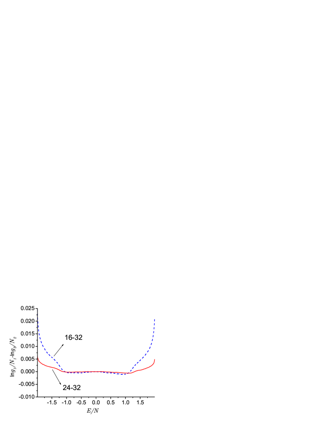
Figure 2: The difference of two dimensional XY model on square lattices of size $16\times 16$ and $32\times 32$, and $24\times 24$ and $32\times 32$ after scaling. The DOS of energy $E=0$ is adjusted so that they have the same value.

With the above mentioned method, we simulated the relative DOS for each enlarged sub-intervals of the middle part, and evaluated the DOS close to the spectrum boundaries by the analytic expressions. Since each sub-interval is enlarged a little bit so that there is a overlap region at each join part, this overlap can help to get a smooth connect with high accuracy. We also take consideration of the trick of Shulz et alBKMD2003PRE in the accurate calculation of the DOS on the interval boundaries. The final result of DOS is shown in Fig. 1. The calculation are performed with finite systems of $16\times 16$, $24\times 24$ and $32\times 32$, and periodical boundary condition were used in the simulation. The DOS shows the generic behavior: $g(E,N){\sim}e^{N{\phi}(E/N)}$ where ${\phi}(E/N)$ is an intensive function. This behavior is consistent with the scaling law in ref.RRA2002PA ; R2004JSP ; RR1999PRL . It should be noted that this scaling relation is strictly satisfied only in the thermodynamic limit where $N\to\infty$. In Fig. 2 we show the small deviations of $\ln g_{16\times 16}/N$ and $\ln g_{24\times 24}/N$ to $\ln g_{32\times 32}/N$ with respect to $E/N$. From the figure we see that the difference between the case of $24\times 24$ and $32\times 32$ is much smaller than the difference between the case of $16\times 16$ and $32\times 32$. Based on this result we expect that the case of $32\times 32$ is a very good approximation to the infinite system, and the DOS calculated with $32\times 32$ should be good enough in most applications. However, in the case a phase transition is occurred the finite size effect may be important and the $32\times 32$ lattice may be too small to obtain accurate results as in the case of KT transition.

II.2 thermodynamic quantities

With the accurate result of the DOS obtained, some thermodynamic quantities can be calculated from it by a simple integration. The internal energy, the specific heat, the free energy and entropy can be immediately calculated according to the equations as follows:

$$U(T) =\frac{{\sum_{E}}Eg(E)e^{-{\beta}E}}{{\sum_{E}}g(E)e^{-{\beta}E}}=\langle E\rangle_{T}$$ (8)

$$C(T) =\frac{{\partial}U}{{\partial}T}=\frac{\langle E^{2}\rangle_{T}-{\langle E\rangle^{2}}_{T}}{T^{2}}$$ (9)

$$Z ={\sum_{E}}g(E)^{-{\beta}E}$$ (10)

$$F(T) =-T\ln Z$$ (11)

$$S(T) =\frac{U(T)-F(T)}{T}$$ (12)

From the expression we see that the partition function can not be obtained without the knowledge of the normalization constant $C$, and neither of the free energy and the entropy. When the temperature $T\rightarrow 0$ we may use Eq. (6) to get the analytic expressions of thermodynamic quantities at low temperature:

$$Z ={\int^{-2N}_{2N}}C(E+2N)^{\frac{N-3}{2}}e^{-{\frac{E}{T}}}dE=C{\Gamma}\left(\frac{N}{2}\right)e^{\frac{2N}{T}}T^{\frac{N-1}{2}}$$ (13)

$$F =-T\ln Z=-T\ln\left[C{\Gamma}\left(\frac{N}{2}\right)\right]-2N-{\frac{N-1}{2}}T\ln T$$ (14)

$$S =-\frac{{\partial}F}{{\partial}T}=\ln\left[C{\Gamma}\left(\frac{N}{2}\right)\right]+{\frac{N-1}{2}}\left(\ln T+1\right)$$ (15)

$$C =T\frac{{\partial}S}{{\partial}T}=\frac{N-1}{2}$$ (16)

$$U =F+TS=-2N+\frac{N-1}{2}T$$ (17)

The low temperature result was obtained in the assumption that the total number of lattice sites is very large, that is, the thermodynamic limit $N\rightarrow\infty$ is assumed. By taking the the zero temperature limit we get the ground state behavior: $F\rightarrow-2N$, $S\rightarrow-\infty$, $C\rightarrow\frac{N}{2}$ and $U\rightarrow-2N$. The behavior of the entropy does not follow the third law of thermodynamics, which requires that the entropy is zero in the limit. The reason for this discrepancy is the ignorance of the quantum effect of our calculation, in fact, in real physical systems the zero temperature behavior of the system is always quantum. Mathematically the incorrect zero temperature limit of entropy comes from the finite and continuous density of states close to the ground state. The zero temperature entropy is given by $S(T=0)=\ln g_{0}$, where $g_{0}$ is the degeneracy of the ground state. For XY model, the density of states is continuous so that the number of states at any specific point of energy is zero, thus $g_{0}=0$ and $S\to-\infty$.

The results of the thermodynamical quantities in a large temperature range was evaluated by numerical integration and are shown in Fig. 3. The figures plot the quantities per site for different sizes of the system, and it is clear from the figures that the results of different sizes of the lattices basically follow the same curve, which indicates that the size effect is not quite important for system size larger than $16\times 16$, the smallest system we calculated.

As we only consider short range interaction, this result is consistent with ref.RRA2002PA ; R2004JSP ; RR1999PRL . The peak of the specific heat differs with the size of the system. In the temperature near $T=1$, the entropy shows a sudden rise, which indicates the rise of the number of microscopic configurations. We know in the temperature of KT transition the vortex pairs break up and the restrict is releasedJV1979PRB , which also gives a rise to the number of microscopic configurations. So the abnormal behavior of the entropy curve may probably show the KT transition. As KT transition is very weak, it can hardly be observed from the free energy curve. It is known that the effective vortex pair interaction is long ranged so that our current system size is too small to describe the KT transition properly. Thus the accurate transition temperature is yet not determined by this method.

III CONCLUSIONS

We calculated the DOS of two dimensional XY model on a square lattice by using the Wang-Landau algorithm combined with analytical expressions on the spectrum boundaries. And from the DOS we calculated the internal energy, the specific heat, the free energy and the entropy. From the curve of entropy we see some symptoms of phase transition. We find that simulation algorithms will meet difficulties in the calculation of DOS close to the spectrum boundaries with continuous models. We propose a general method to solve such difficulty by using the analytical expressions at the boundaries.

This work is supported by the National Nature Science Foundation of China under grant #10334020 and #90103035 and in part by the National Minister of Education Program for Changjiang Scholars and Innovative Research Team in University.

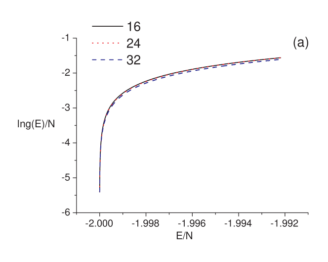
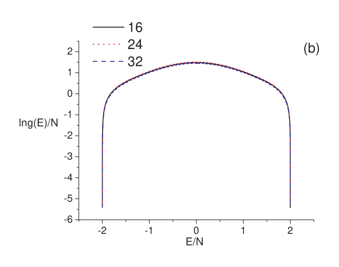
Figure 1: (a) the density of states near the lowest energy of two dimensional XY model on square lattices of size $16\times 16$, $24\times 24$, $32\times 32$. (b) the density of states in the whole energy range of two dimensional XY model on square lattices of size $16\times 16$, $24\times 24$, $32\times 32$.

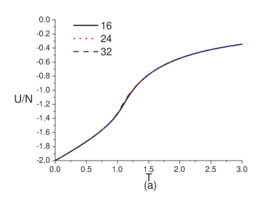
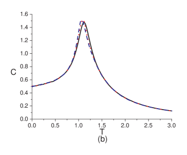
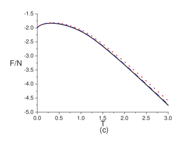
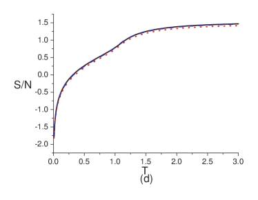
Figure 3: The internal energy, specific heat, free energy and entropy of the two dimensional XY model on square lattices. $16\times 16$ solid line, $24\times 24$ dot line and $32\times 32$ dash line.

References

- (1) R.Salazar,R.Toral and A.R.Plastino, Physica A 305, 144 2002
- (2) R.Toral, J. Stat. Phys. 114, 516 2004
- (3) Jan Tobochnik and G.V.chester, Phys. Rev. B. 20, 9 (1979)
- (4) Fugao Wang and D.P.Landau, Phys. Rev. Lett. 86, 10 (2001)
- (5) Fugao Wang and D.P.Landau, Phys. Rev. E. 64, 050101 (2001)
- (6) Chenggang Zhou and R.N.Bhatt, Phys. Rev. E. 72, 025701 (2005)
- (7) B.J.Shulz,K.Binder,M.Müller,and D.P.Landau, Phys. Rev. E. 67, 067102 (2003)
- (8) R.Salazar,R.Toral, Phys. Rev. Lett. 83, 4233 (1999)