Universal velocity distributions in an experimental granular fluid

Abstract

We present experimental results on the velocity statistics of a uniformly heated granular fluid, in a quasi-2D configuration. We find the base state, as measured by the single particle velocity distribution $P(c)$, to be universal over a wide range of filling fractions and only weakly dependent on all other system parameters. There is a consistent overpopulation in the distribution’s tails, which scale as $P\propto\exp(\mathrm{-A}\times c^{-3/2})$. More generally, $P(c)$ deviates from a Maxwell-Boltzmann by a second order Sonine polynomial with a single adjustable parameter, in agreement with recent theoretical analysis of inelastic hard spheres driven by a stochastic thermostat. To our knowledge, this is the first time that Sonine deviations have been measured in an experimental system.

I Introduction

The study of granular flows has received a recent upsurge of interest in physicsJaeger et al. (1996). This has been motivated by both the relevance of such flows to a wide range of industrial and geological processes, and by the realization that granular materials provide an excellent test bed for a number of fundamental question in the context of modern fluid dynamics and non-equilibrium statistical mechanics Kadanoff (1999). Granular media are ensembles of macroscopic particles, in which kinetic energy ($K_{E}$) can be preferentially injected in the $N\simeq 10-10^{10}$ translational and rotational degrees of freedom of the center of mass of the particles without effecting the $N_{A}\simeq 10^{23}$ internal degrees of freedom of each particle. Therefore the granular temperature $T=K_{E}/N$ is $10-20$ orders of magnitude larger than the molecular temperature $\tau=K_{E}/N_{A}$. In this sense the molecular temperature is irrelevent. Moreover, granular materials are intrinsically dissipative since energy from the $K_{E}$ of the particles is lost (converted) through inelastic collisions and frictional contacts to the molecular temperature. Hence, any dynamical study of a granular media requires an energy input, which typically takes the form of vibration or shearMelo et al. (1994); Miller et al. (1996). This interplay between energy injection and dissipation forces the system to be far from equilibrium and granular fluids are therefore not expected to behave similarly to the equilibrium counter-parts of classical fluidsKadanoff (1999).

However, we have recently shown that the structure of a uniformly heated quasi-2D granular fluid is identical to that found in simulations of equilibrium hard disksReis et al. (2006a). Further, we find that the mean-squared displacement of grains shows diffusive behavior at low density and caging behavior as density is increased until particles are completely confined above freezing point just as in ordinary molecular fluidsReis et al. (2006b). These surprising results provide a partial experimental justification for the theoretical treatment of granular flow by analogy with molecular fluids using standard statistical mechanics and kinetic theory. A large number of kinetic theories of granular flowsSavage and Jeffery (1981); Lun et al. (1983); Jenkins and Richman (1985a); Jenkins and Richman (1985b, 1988); Lun (1991); Goldshtein and Shapiro (1995a); Sela et al. (1996); Brey et al. (1996); Santos et al. (1998); van Noije et al. (1998a); Garzó and Dufty (1999); Dufty and Brey (2003); Brey and Ruiz-Montero (2004); Dufty et al. (2004); Kumaran (2005); Brey and Dufty (2005); Lutsko (2006) have been produced starting in 1980’s. The results of these theories are balance equation analogous to the Navier-Stokes equations for the density, $n$, the average velocity, $\mathbf{v}_{o}$, and the average kinetic energy per particle or temperature, $T$, as well as, equations of state and transport coefficients, which are functions of $n$,$\mathbf{v}_{0}$, and $T$. The heart of these formulations is the single particle distribution function $f^{(1)}\left(\mathbf{r},\mathbf{v},t\right)$, which measures the probability of a particle a position $\mathbf{r}$ having velocity $\mathbf{v}$. The field equations are derived from moments of $f^{(1)}\left(\mathbf{r},\mathbf{v},t\right)$. For example, the density, $n$, is the 0th moment, the average velocity, $\mathbf{v}_{o}$, is the 1st moment, and the temperature, $T$, is the 2nd moment. The transport coefficients are deterimined from non-equilibrium perturbations of $f^{(1)}\left(\mathbf{r},\mathbf{v},t\right)$. Generally the equilibrium or steady-state distribution is assumed to be indepent of space and to have Maxwell-Boltzmann form $f^{(1)}=f_{MB}=A\exp\left(-\frac{|\mathbf{v}-\mathbf{v}_{0}|^{2}}{2T}\right)$, although, recent work has explored the use of other base states or steady-state distributions Dufty et al. (2004); Brey and Dufty (2005); Lutsko (2006).

Two important questions one may ask are: 1) What is the base state $f^{(1)}$ for a driven granular fluid? and 2) Does it have a universal form?. If it is characterized by a small number of parameters such as the moments of the $f^{(1)}$ distribution as in the case for ideal fluids, one would be able to advance a great deal in developing predictive continuum models for granular flows since the theoretical machinery from kinetic theory could be readily applied. The careful experimental study and characterization of this base state is therefore important in order to develop a theory for granular media similar to that of regular molecular liquids.

There has been a substantial amount of experimental, numerical, and theoretical work to address these issues in configurations where the energy input perfectly balances the dissipation such that the system reaches a steady state, albeit far from equilibrium. These non-equilibrium steady states are simplified realizations of granular flows more amenable to analysis, but the insight gained from their study should be helpful in the tackling of other more complex scenarios. One feature that has been consistantly established in experiments is that single particle velocity distribution functions deviate from the Maxwell-Boltzmann distribution Losert et al. (1999); Olafsen and Urbach (1999); Rouyer and Menon (2000); Blair and Kudrolli (2001); Prevost et al. (2002); Aranson and Olafsen (2002); Blair and Kudrolli (2003). In particular, the tails (i.e. large velocities) of the experimental distributions exhibit a considerable overpopulation and have been shown to scale as $f^{(1)}(v_{i})\sim\exp[(v_{i}/\sqrt{T_{i}})^{3/2}]$ where $v_{i}$ is a velocity component and $T_{i}=\langle v_{i}^{2}\rangle$ is the granular temperature. This behavior is in good agreement with both numerical Moon et al. (2001) and theoretical van Noije and Ernst (1998) predictions. Even though the tails correspond to events with extremely low probabilities, they increase the variance of the distribution. The variance of the distribution is $T$, the average kinetic energy of the particles. Using a Gaussian to represent this type of distribution leads to major discrepancy in the region of high probability at the central part of the distribution (low velocities) Blair and Kudrolli (2003) which have, thus far, been greatly overlooked in experimental work. Note that requiring the variance of $f^{(1)}(v_{i})$ to be the granular temperature greatly constrains the functional form that the distribution can take.

A model system that has been introduced to study this question is the case of a homogeneous granular gas heated by a stochastic thermostat, i.e. an ensemble of inelastic particles randomly driven by a white noise energy source Williams and MacKintosh (1996). Recently, there have been many theoretical and numerical studies on this model system van Noije and Ernst (1998); van Noije et al. (1999); Montanero and Santos (2000); Moon et al. (2001); Brilliantov and Poschel (2006); Pöschel et al. (2006) where the steady state velocity distribution have been found to deviate from the Maxwell-Boltzmann distribution. van Noije and Ernst van Noije and Ernst (1998) studied these velocity distributions based on approximate solutions to the inelastic hard sphere Enskog-Boltzmann equation by an expansion in Sonine polynomials. The results of their theoretical analysis has been validated by numerical studies using both molecular dynamics Moon et al. (2001) simulations and direct simulation Monte Carlo Montanero and Santos (2000); Pöschel et al. (2006). The use Sonine corrections is particular attractive since it leaves the variance of the resulting velocity distribution unchanged but leads to a non-Gaussian fourth moment or kurtosis $K\neq 3$.

We have addressed the above issues in a well controlled experiment in which we are able to perform precision measurements of the velocity distributions of a uniformly heated granular fluid. A novel feature of our experimental technique is that we are able to generate macroscopic random walkers over a wide range of filling fractions and thermalize the granular particles in a way analogous to a stochastic thermostat. This is an ideal system to test the applicability of some of the kinetic theory ideas mentioned above. In our earlier study Reis et al. (2006a), we focused on the structural configurations of this granular fluid and revealed striking similarity to those adopted by a fluid of equilibrium hard disks. Here we concentrate on the dynamical aspects of this same experimental system, as measured by the single particle velocity distribution, $P(c)$, and observe a marked departure from the equilibrium behavior, i.e. from the Maxwell-Botlzmann distribution. We quantify these deviations from equilibrium and show that they closely follow the predictions, in the kinetic theory framework, of the theoretical and numerical work mentioned above. In particular, we find a consistent overpopulation in the distribution’s high energy tails, which scale as stretched exponentials with exponent $-3/2$. In addition, we experimentally determine the deviations from a Gaussian of the full distributions using a Sonine expansion method and find them to be well described by a second order Sonine polynomial correction. We establish that the entire experimental velocity distribution functions are universal and well described by

$$P(c)=f_{MB}\left(1+a_{2}(1/2c^{4}-3/2^{2}+3/8)\right)$$ (1)

where $a_{2}$ is the non-gaussianity parameter that can be related to the Kurtosis of the distribution and the forth-order polynomial is the Sonine polynomial of order 2. This functional form of $P(c)$ was found to be valid over a wide range of the system parameters. To our knowledge, this is the first time that the Sonine corrections of the velocity distributions are measured in an experimental system, in agreement with analytical predictions.

This paper is organized as follows. In Sec. II we briefly review the theoretical framework of kinetic theory along with the steady state solution to the Enskog-Boltzmann equation using the Sonine polynomial expansion method. In Sec. III we present our experimental apparatus and describe how the homogeneous granular gas with random heating is generated. In Sec. IV we study the thermalization mechanism by analyzing the trajectories of a single particle in the granular cell. In Sec., V, using the concept of granular temperature, we then quantify the dynamics of the experimentally obtained non-equilibrium steady states, for a number of parameters, namely: the filling fraction, the driving parameters (frequency and acceleration) and the vertical gap of the cell. In Sec. VI we turn to a detailed investigation of the Probability Distribution Functions of velocities as a function of the system parameters. In particular, we quantify the deviations from Maxwell-Boltzmann behavior at large velocities (tails of the distributions) – Sec. VI.1. In Sec. VI.2 we extend the deviation analysis to the full range of the distribution using an expansion method that highlights deviations at low velocities and allows us to make a connection with Sonine polynomials. We finish in Sec. VII with some concluding remarks.

II Brief Review of Theory

We briefly review the key features of the kinetic theory for granular media pertinent to our study. The number of particles in a volume element, dr, and velocity element, dv, centered at position r and velocity v is given by $f^{1}(\textbf{r},\textbf{v},t)\textsl{d}\textbf{r}\textsl{d}\textbf{v}$, where $f^{1}(\textbf{r},\textbf{v},t)$ is the single particle distribution function. Continuum fields are given as averages over $f^{1}(\textbf{r},\textbf{v},t)$. For instance, the number density, $n$, average velocity, $v_{o}$, and granular temperature, $T$, are given respectively by,

$$n(\textbf{r},t)\equiv\int f^{1}(\textbf{r},\textbf{v},t)\textsl{d}\textbf{v},$$ (2)

$$\textbf{v}_{o}(\textbf{r},t)\equiv\frac{1}{n}\int f^{1}(\textbf{r},\textbf{v},t)\textbf{v}\textsl{d}\textbf{v},$$ (3)

$$T(\textbf{r},t)\equiv\frac{1}{nd}\int f^{1}(\textbf{r},\textbf{v},t)(\textbf{v}-\textbf{v}_{o})^{2}\textsl{d}\textbf{v},$$ (4)

where $d$ is the number of dimensions. It is important to note that the granular temperature $T$ is not the thermodynamic temperature but, by analogy, the kinetic energy per macroscopic particles (explained in detail in Sec. V). For the spatially homogeneous and isotropic case, we refer to the single particle distribution function as $f^{1}(\textbf{v},t)$ and consider only a single component of the velocity, i.e. $f^{(1)}(v_{i},t)$. From now on we drop the index $i$. It is also convenient to introduce a scaled distribution function $f^{1}(c,t)$ where the velocity is scaled by a characteristic velocity such that, $c=v/\sqrt{2T(t)}$, where $T(t)$ is the granular temperature and equal to the variance of $f^{1}(c,t)$.

The stocastically heated single particle distribution function $f(c,t)$ satisfies the Enskog-Boltzmann equation,

$$\frac{\partial f}{\partial t}=\mathcal{Q}(f,f)+\mathcal{F}_{FP}f,$$ (5)

where, $\mathcal{Q}$, is the collision operator, which accounts for the inelastic particle interactions and the Fokker-Plank operator, $\mathcal{F}_{FP}$, accounts for the stochastic forcing van Noije and Ernst (1998); van Noije et al. (1998b). We are interested in a stationary solution of Eqn. (5) where the heating exactly balances the loss of energy due to collisions and the temperature becomes time independent. van Noije and Ernst van Noije and Ernst (1998) obtained steady state solutions to Eqn. (5) by taking the series expansion of $f(c)$ away from a Maxwell-Boltzmann, $f_{MB}$, i.e.

$$f(c)=f_{MB}(c)\left\{1+\sum_{p=1}^{\infty}a_{p}S_{p}(c^{2})\right\},$$ (6)

in terms of the Sonine polynomials $S_{p}(c^{2})$ where $a_{p}$ is a numerical coefficient for the $p^{th}$-order. The deviations from the MB distribution are thus expressed in terms of an expansion on Sonine polynomials. The Sonine polynomials, which are knows as associated Laguerre polynomials in different contexts, are defined as,

$$S_{p}(c^{2})=\sum_{n=0}^{p}\frac{(-1)^{n}(p+1/2)!}{(n+1/2)!(p-n)!n!}(c^{2})^{n}.$$ (7)

These are orthogonal accordingly to the relationship,

$$\int_{0}^{\infty}c^{2}e^{-c^{2}}S_{p}(c^{2})S_{m}(c^{2})\textit{dc}=\frac{1}{2}\delta_{pm}\frac{(\frac{1}{2}+n)!}{n!}.$$ (8)

To further simply the calculation, terms higher than $\mathcal{O}(2)$ are typically neglected, such that,

$$f(c)=f_{MB}(c)\left\{1+a_{2}S_{2}(c^{2})\right\},$$ (9)

where,

$$f_{MB}(c)=\frac{1}{\sqrt{\pi}}exp(-c^{2}),$$ (10)

is the Maxwell-Boltzmann distribution and

$$S_{2}(c^{2})=\frac{1}{2}c^{4}-\frac{3}{2}c^{2}+\frac{3}{8}$$ (11)

is the $\mathcal{O}(2)$ Sonine polynomial for 2D. The first Sonine coefficient, $a_{1}$, is zero according to the definition of temperature Goldshtein and Shapiro (1995b). The second Sonine coefficient, $a_{2}$ is the first non-trivial Sonine coefficient and hence the first non-vanishing correction to the MB distribution and can be related to the Kurtosis $K=3(a_{2}+1)$ of the distribution.

III Our experiments

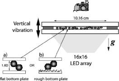
Figure 1: Schematic diagram of the experimental apparatus. The ensemble of stainless steel spheres was sandwiched in between two glass plates, separated by a $1.905mm$ thick annulus (dark grey). Top glass plate was always optically flat. Bottom glass plate could either be (a) optically flat or (b) rough by sand-blasting.

In Fig. 1 we present a schematic diagram of our experimental apparatus, which is adapted from a design introduced by Olafson and Urbach Olafsen and Urbach (1999); Prevost et al. (2002). An ensemble of stainless steel spheres (diameter $D=1.19mm$) were vertically vibrated in a shallow cylindrical cell, at constant volume conditions. The cell consisted of two parallel glass plates set horizontally and separated by a stainless steel annulus. This annulus had an inner diameter of $101.6mm$ and, unless otherwise stated, was $1.905mm$ thick, which set the height of the cell to be 1.6 particle diameters. This constrained the system to be quasi-two dimensional such that each sphere could not fully overlap. However the 2D projection of the particles have a minimum separation of $r_{min}=0.8D$ (rather than $r_{min}=D$ for a strictly two-dimensional system). Hence, the extreme situation of a maximum overlap between two particles ($\delta=D-r_{min}=0.2D$) occurred when one of the particles of the adjacent pair was in contact with the bottom plate and the other in contact with the top plate, as shown in Fig. 1(a). We have also performed experiments to explore the effect of changing the height of the cell.

The top disk of the cell was made out of an optically flat borofloat glass treated with a conducting coating of ITO to eliminate electrostatic effects. For the bottom disk of the cell, two variants were considered: a flat glass plate identical to the top disk – Fig. 1(a) – and a rough borosilicate glass plate – Fig. 1(b). In the second case, the plate was roughened by sand-blasting, generating random structures with lengthscales in the range of $50$–$500\mu m$. The use of a rough bottom glass plate improves on the setup of Olafsen and Urbach Olafsen and Urbach (1999), who used a flat plate. As it will be shown in Sec. IV and Appendix A, it had the considerable advantage of effectively randomizing the trajectories of single particles under vibration, allowing a considerably wider range of filling fractions to be explored.

The horizontal experimental cell was vertically vibrated, sinusoidally, via an electromagnetic shaker (VG100-6 Vibration Test System). The connection of the shaker to the cell was done via a robust rectangular linear air-bearing which constrained the motion to be unidirectional. The air-bearing ensured filtering of undesirable harmonics and non-vertical vibrations due to its high stiffness provided by high-pressure air flow in between the bearing surfaces. Moreover, the coupling between the air-bearing and the shaker consisted of a thin brass rod ($25.4mm$ long and $1.6mm$ diameter). This rod could slightly flex to correct any misalignment present in the shaker/bearing system, while being sufficiently rigid in the vertical direction to fully transmit the motion. This ensemble – shaker/brass rod/air-bearing – ensured a high precision vertical oscillatory driving.

The forcing parameters of the system were the frequency, $f$, and amplitude, $A$, of the sinusoidal oscillations. From these, it is common practice to construct a non-dimensional acceleration parameter,

$$\Gamma=\frac{A(2\pi f)^{2}}{g},$$ (12)

where $g$ is the gravitational acceleration. We worked within the experimental ranges $(10<f<100)Hz$ and $1<\Gamma<6$. The first control parameter was the filling fraction of the steel spheres in the cell defined as,

$$\phi=\frac{N\pi(D/2)^{2}}{\pi R^{2}},$$ (13)

where $N$ is the number of spheres (with diameter $D=1.19mm$) in the cell of radius $R=50.8mm$. The filling fraction $\phi$ is therefore defined in the projection of the cell onto the horizontal plane. The second control parameter was the height, $h$, of the experimental cell which we varied from $1.3D<h<2.3D$.

The granular cell was set horizontal in order to minimize compaction effects, inhomogeneities and density gradients which otherwise would be induced by gravity. This way, a wide range of filling fractions, $0<\phi\leq 0.8$, could be accurately explored by varying the number of spheres in the cell, $N$, down to a resolution of single particle increments. Moreover, as we shall show in Sec. IV–V, we were able to attain spatially uniform driving of the spheres in the cell due to the use of the rough glass bottom plate.

The dynamics of the system was imaged from above by digital photography using a grayscale DALSA CA-D6 fast camera, at 840 frames per second. The granular layer was illuminated from below, in a transmission configuration, by a $16\times 16$ array of high intensity LEDs. In this arrangement the particles obstruct the light source and appear as dark circles in a bright background.

We have developed particle tracking software based on a two-dimensional least squares minimization of the individual particle positions, which is able to resolve position to sub-pixel accuracy. By focusing on a $(15\times 15)mm^{2}$ imaging window located in the central region of the full cell we were typically able to achieve resolutions of 1/20–1/10 of a pixel (which corresponds to $2.5$–$5\mu m$). From the trajectories of the particles we could easily calculate an approximately instantaneous discretized velocity as,

$$|v^{i}(t_{j}+\Delta t)|=\sqrt{(v_{x}(t_{j}+\Delta t))^{2}+v_{y}((t_{j}+\Delta t))^{2}}$$ (14)

with

$$v_{x}=\frac{x^{i}(t_{j}+\Delta t)-x^{i}(t)}{\Delta t}\quad\mathrm{and}\quad v_{y}=\frac{y^{i}(t_{j}+\Delta t)-y^{i}(t)}{\Delta t}$$ (15)

for the $i^{th}$ particle in an experimental frame at time $t_{j}$ where $\Delta t=1.19\mu s$ is the time interval between two frames and $(x,y)$ are the cartesian coordinates on the horizontal plane. For the remainder of this paper we shall be interested in the nature of the probability distribution function of velocities, $P(v)$, of the driven particles. Statistics for calculating the $P(v)$ distributions were constructed by analyzing 2048 frames at an acquisition rate of 840 frames per second which corresponded to an acquisition real time of $2.4381s$.

IV Single particle driving

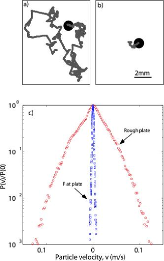
Figure 2: Typical trajectories for single particle driven using a (a) rough or (b) flat bottom glass plate. Each of the trajectories is $2.438s$ long. (c) Probability distribution function of velocities for a single particles using rough ($\circ$) and flat ($\square$) bottom glass plate. Driving parameters: $f=50Hz$, $\Gamma=4.0$.

We first concentrate on the case of the driving of a single particle in the vibrating experimental cell. For each experimental run, a single sphere was positioned in the field of view of the camera with the aid of a strong magnet temporarily placed beneath the imaging window. The magnet was then removed and the trajectory of the sphere immediately recorded. This was repeated 100 times to obtain statistics. Typical trajectories for two runs with a flat and rough bottom glass plates are shown in Fig. 2(a) and (b), respectively. In both cases, the cell was vibrated at a frequency of $f=50Hz$ and dimensionless acceleration of $\Gamma=4.0$. During each cycle of the driving, the motion of the single particle was thermalized due to collisions with both top and bottom glass plates.

By comparing Fig. 2(a) with Fig. 2(b), it is clear that the particle excursions obtained by using a rough bottom plate are considerable larger than those for a flat plate. This can be readily quantified by calculating the Probability Density Functions of the velocities of single particles, $P(v)$, which we plot in Fig. 2(c), for both cases. We now define the average kinetic energy, also known as granular temperature, of a single particle as the variance of its velocity distribution,

$$T=T_{x}+T_{y}=\frac{1}{2}\left(\langle v_{x}^{2}\rangle+\langle v_{y}^{2}\rangle\right),$$ (16)

where $v_{x}$ and $v_{y}$ are the two orthogonal components of the velocity in the 2D horizontal plane and the brackets $\langle.\rangle$ denote time averages for the timeseries of the velocity components for 100 particle trajectories. Note that since we are dealing with monodisperse spheres, in this definition of kinetic temperature, the mass of the particle is taken to be unity. We have measured $T^{s}_{rough}=9.53\times 10^{-4}m^{2}s^{-2}$ if a rough bottom glass plate is used and $T^{s}_{flat}=2.51\times 10^{-6}m^{2}s^{-2}$ for the case of the flat bottom glass plate. This yields a temperature ratio between the two cases of $T^{s}_{rough}/T^{s}_{flat}=380$.

Indeed, this is a signature that the structures in the rough plate were considerably more effective than the flat plate in transferring and randomizing the momentum of the steel spheres in the vertical direction (due to the sinusoidal vertical oscillation of the cell) into the horizontal plane. The velocity of the steel sphere was randomized each time it collided with the peaks and valleys randomly distributed across the the sand-blasted rough glass surface. We can therefore regard this system as a spatially uniform heater of the granular particles, thereby generating macroscopic random walkers. For this reason, and as it will become more clear in the next Sec., where we will further comment on the issue of isotropy, we shall focus our experimental study in using the rough bottom glass plate.

V Driven monolayers: granular temperature

a)	b)	c)

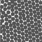
Figure 3: Snapshots of typical configurations of the granular layer at various values of the filling fraction: (a) dilute gas, $\phi=0.34$, (b) dense liquid, $\phi=0.67$ and (c) thermalized crystal, $\phi=0.80$. Driving parameters: $f=50Hz$, $\Gamma=4.0$.

Having investigated the dynamics of single particles in the granular cell, we now turn to the study of granular monolayers at higher filling fractions. In Fig. 3 we present typical configurations, at three values of $\phi$, for a granular layer driven at $f=50Hz$ and $\Gamma=4$ with a rough bottom plate. The snap-shot in Fig. 3(a), for $\phi=0.34$, corresponds to a dilute state in which the particles perform large excursions in between collisions as they randomly diffuse across the cell. If the filling fraction is increased, as in the example of the frame shown in Fig. 3(b) for $\phi=0.67$, one observes a higher collision rate characteristic of a dense gaseous regime. For even higher values of filling fraction the spheres ordered into an hexagonally packed arrangement and became locked into the cage formed by its six neighbors. The system is then said to be crystalized as shown in the typical frame presented in Fig. 3(c) for $\phi=0.80$. The structural configurations associated with the crystallization transition, as a function of filling fraction, were studied in detail in Reis et al. (2006a) and the caging dynamics, as crystallization is approached in Reis et al. (2006b).

As defined in the previous section the granular temperature is the average kinetic energy per particle. For this the brackets $\langle.\rangle$ in Eqn. (16) now denote both time and ensemble averages for all the spheres found within the imaging window. Moreover, one can define $T_{x}=1/2\langle v_{x}^{2}\rangle$ and $T_{y}=1/2\langle v_{y}^{2}\rangle$, with $T=T_{x}+T_{y}$, as the temperature projections onto the $x$ and $y$ directions of the horizontal plane.

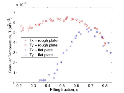
Figure 4: Filling fraction dependence of the granular temperature ($T_{x}$ and $T_{y}$ are the $x$ and $y$ components, respectively), for both cases of using a flat and rough bottom glass plates. Driving parameters: $f=50Hz$ and $\Gamma=4.0$.

In Fig. 4 the temperature components, $T_{x}$ and $T_{y}$, are plotted as a function of filling fraction. For both cases of using a rough and a flat bottom plate, the respective $T_{x}$ and $T_{y}$ are identical. This shows that the forcing of the granular particles was isotropic. In agreement with the case of a single particle, the dynamics of the granular layer using a flat or a rough bottom plate is remarkably different. If the rough bottom plate is used, the granular temperature depends almost monotonically on the filling fraction. At low $\phi$, $T$ is approximately constant as the layer simply feels the thermal bath and shows little increase in $T$ until $\phi\sim 0.5$ is reached. As the filling fraction is increased past $\phi\sim 0.5$, the granular temperature rapidly decreases due to energy loss in the increasing number of collisions and due to a decreasing available volume.

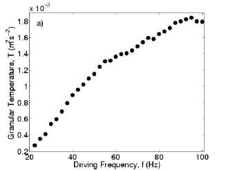
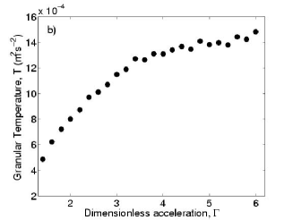
Figure 5: Dependence of the granular temperature, $T$, on driving parameters: (a) frequency, $f$ and (b) dimensionless acceleration $\Gamma$. The filling fraction is kept constant at $\phi=0.59$.

For the case of using a flat bottom plate, the non-monotonic dependence of $T$ on $\phi$ is more dramatic and it is difficult to attain homogeneous states below $\phi<0.4$. This is due to the fact that at those filling fractions (the limiting case being the single particle investigated in the previous section) the particles perform small excursions and interact with their neighbors only sporadically. Hence, little momentum is transferred onto the horizontal plane. For $\phi>0.5$, there is an increase of temperature with increasing filling fraction as interaction between neighbors becomes increasingly more common up to $\phi\sim 0.7$ at which the curve for the flat bottom plate coincides with the curve for the rough bottom plate. It is interesting to note that the value at which this matching occurs is close to the point of crystallization of disks in 2D, $\phi_{c}=0.716$ Alder and Wainwright (1962); Mitus et al. (1997); Reis et al. (2006a). At this point, the large number of collisions between neighboring particles thermalizes the particles, independently of the details of the heating, i.e. of whether a flat or rough plate is used.

The behavior of the layer was therefore more robust by using a rough bottom plate. Moreover, this allowed for a wider range of filling fractions to be explored, in particular in the low $\phi$ limit. Further detailed evidence for the advantage of using the rough bottom plate over a flat one is given in Appendix A. Hence, all results presented in the remainder of this paper correspond to experiments for which a rough glass plate was used for the bottom plate of the experimental cell.

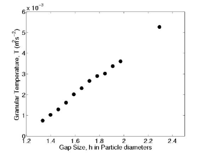
Figure 6: Dependence of the granular temperature, $T$, on cell gap, $h$, which was varied by changing the thickness of the inter-plate annulus. Filling fraction was kept constant at $\phi$=0.59 and the dimensionless acceleration $\Gamma$ was fixed to 4.

In Fig. 5 we present the dependence of the granular temperature of the layer on the forcing parameters for a fixed value of filling fraction, $\phi=0.59$. There is a monotonic increase of $T$ with both $f$ and $\Gamma$.

The final control parameter that we investigated was the height of the experimental cell which we varied by changing the thickness of the inter-plate annulus by using precision spacers. The range explored was $1.3D<h<2.3D$. Note that for $h=D$ there would be no clearance between the spheres and the glass plates and one would therefore expect for no energy to be injected into the system. On the other hand for $h>2D$, spheres could overlap over leach other and the system ceases to be quasi-2D. The dependence of the granular temperature on cell gap is plotted in Fig. 6. It is interesting to note that $T$ appears to depend linearly on the gap height.

One can therefore regard changing $h$, $f$ and $\Gamma$ as a way of varying the temperature of the granular fluid, which can this way be tuned up to a factor of eight.

VI Probability density functions of velocities

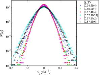
Figure 7: (a) Probability distribution function of velocities (PDF), $P(v)$, for specific values of filling fraction ($\phi$), frequency ($f$) and dimensionless acceleration ($\Gamma$). See legend for specific values.

We now turn to the distribution functions of particle velocities under various conditions of filling fraction, frequency, dimensionless acceleration and gap height. In Fig. 7 we plot the probability density function of a velocity component, $P(v_{i})$, where the index $i$ represents the component $x$ or $y$, for specific values of $\phi$, $f$ and $\Gamma$. From now on we drop the index in $v_{i}$ since we showed in the previous section that the dynamics of the system is isotropic in $x$ and $y$. Moreover, when we refer to velocity we shall mean velocity component, $i$. The width of the observed $P(v)$ differs for various values of the parameters. This is analogous to the fact that the temperature (i.e. the variance of the distribution) is different for various states set by $\phi$, $f$ and $\Gamma$, as discussed in the previous Sec.. It is remarkable, however, that all the $P(v)$ distributions can be collapsed if the velocities are normalized by the characteristic velocity,

$$v_{o}=\sqrt{2\langle v^{2}\rangle}=\sqrt{2T}$$ (17)

where the brackets $\langle.\rangle$ represent time and ensemble averaging over all the particles in the field of view of the imaging window. This collapse is shown in Figs. 8(a) and (b) and was accomplished not only for various filling fractions but also for a range of frequencies and dimensionless accelerations.

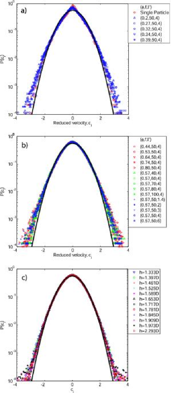
Figure 8: (a)-(b)PDF of velocities, $P(c)$, in which all velocities for each distribution were normalized by its standard deviation. Data for a range of $\phi$, $f$ and $\Gamma$. (c) PDF of velocities for range of values of cell gap, $h$. Other parameters set to $\phi=0.59$, $f=50Hz$ and $\Gamma=4.0$. (a-c) See legend for specific values of the experimental parameters. The solid lines are Gaussian with unit standard deviation.

To highlight the quality of the collapse we have separately plotted $P(c)$ for the four lowest values of filling fraction ($\phi={0.27,0.32,0.34,0.39}$) along with the $P(c)$ for a single particle in Fig. 8(a) and all other data in the ranges $0.44<\phi<0.8$, $40Hz<f<100Hz$ and $1.4<\Gamma<6$ in Fig. 8(b). At low values of the filling fraction ($\phi<0.44$) the collapse is satisfactory but deviations are seen at low $c$. In particular, near $c=0$ the distributions exhibit a sharp peak with a clearly discontinuous first derivative which reflects the fact that for these value of low $\phi$ the resulting gases are not collisionally driven but are dominated instead by the underlying thermostat (c.f. distribution for single particle). However, this sharp peak becomes increasingly smoother as the filling fraction is increased, presumably due to the increasing number of particle collisions, and by $\phi\sim 0.44$, it has practically disappeared. On the other hand, for $\phi>0.44$ the collapse onto a universal curve is remarkable for such a wide range of $\phi$, $f$ and $\Gamma$. The choice of the lower bounds for frequency and acceleration, $f=40Hz$ and $\Gamma=1.4$, in the data plotted will be addressed in Sec. VI.2. Moreover, this collapse of $P(v)$ is also attained for various values of the gap height ($1.3D<h<2.3D$), as shown in Fig. 8(c). From now onwards, we shall perform our analysis in terms of the reduced velocity, $c=v/v_{o}$.

We stress the universal collapse of the experimental velocity distribution functions for a wide range of parameters and the clear deviation from the Maxwell-Boltzmann (Gaussian) distributions of Eqn. (10) – solid curve in Fig. 8(b) and (c). This is particularly visible at high velocities where there is a significant overpopulation of the distribution tails in agreement with previous theoretical van Noije and Ernst (1998), numerical Moon et al. (2001) and other experimental work Rouyer and Menon (2000); Aranson and Olafsen (2002); van Zon et al. (2004). To quantify these deviations from Gaussian behavior, our analysis will be twofold. First we shall analyze the non-Gaussian tails of the velocity distributions (Sec. VI.1). Even though the tails correspond to events associated with large velocity the probability of them happening is extremely low. However, this overpopulation at the tails implies that, if the distribution is to remain normalized with a standard deviation given by the average kinetic energy per particle, clear deviations from Gaussian at the central regions of low $c$ (high probability) of the distribution must necessarily also be observed. In Sec. VI.2 we study this deviations in the context of Sonine corrections introduced in Sec. II.

In Appendix A we provide the data corresponding to Fig. 7 and Figs. 8(a,b) of the velocity distributions obtained using the optically flat bottom plate, instead of the rough plate used here. We shall show that the $P(v)$s for the flat bottom plate exhibit much stronger non-universal deviations from Gaussian behavior and that the collapse of $P(c)$ is highly unsatisfactory. This highlights, as mentioned in Sec. V, the considerable advantage in our experimental technique of using the rough plate to generate the granular fluid.

VI.1 Deviation at large velocities – The tails

Recently, van Noije and Ernst van Noije and Ernst (1998) have made the theoretical prediction that the high energy tails of the velocity distributions of a granular gas heated by a stochastic thermostat should scale as stretched exponentials of the form,

$$P(c)~{}\sim\exp\left(-Ac^{3/2}\right),$$ (18)

where $A$ is a fitting parameter. Note that the theoretical argument of van Noije and Ernst involves a high $c$ limit and hence one does not expect this stretched exponential form to be valid across the whole range of the distribution.

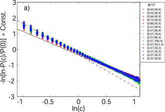
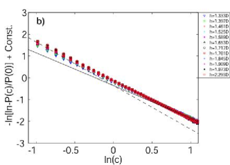
Figure 9: (a) Tails of $P(c)$ for specific values of filling fraction ($\phi$), frequency ($f$) and dimensionless acceleration ($\Gamma$) and (b) gap height ($h$).The solid lines correspond to stretched exponentials of the form $\sim\exp(-Ac^{{3/2}})$ whereas the dashed lines correspond to the Gaussian behavior of the form $\sim\exp(-Ac^{{2}})$.

To check the applicability of Eqn. (18) to describe our data, we have calculated the quantity $q(c)=-\ln\left(-\ln(P(c))\right)$, which we plot in Fig. 9(a) for a variety of filling fractions, frequencies and dimensionless accelerations. Indeed, within the ranges considered and, in the limit of large $c$, $q(c)$ tends to a straight line with slope -3/2 for all values of the control parameters, in excellent agreement with the scaling of Eqn. (18). In Fig. 9(a) we have excluded filling fractions $\phi<0.44$, since as discussed in the previous Sec., the gases obtained in this range are dominated by the thermostat rather than collisions and the main ingredient for the prediction of Eqn. (18) is the role of inelastic collisions. This behavior of the tails of the velocity distribution is also observed for various values of the gap height, $h$, of the experimental cell, as shows in Fig. 9(b). Note the crossover from Gaussian-like (dashed line with slope -2) to the stretched exponential (solid line with slope -3/2) at $c\sim 1$, which is particularly clear at the larger values of $\phi$. For low $\phi$ the tails of the distribution tend to be closer to the stretched exponential throughout the range $-1.1<\log(c)<1.1$. We stress that Eqn. (18) has been derived in the limit of large $c$ and is therefore only expected to be valid at the large $c$ end of the tails. A. Barrat el. al. Barrat and Trizac (2003); Barrat et al. (2005) have investigated the range of validity in a numerical model with a stochastic forcing and found that the stretched exponential scaling of the tails should only be valid for very high velocities corresponding to probabilities lower than $10^{-6}P(0)$. The fact that we find this scaling at considerable lower velocities, i.e. in regions of higher probability, (in agreement with other experimental work Rouyer and Menon (2000)) raises some questions regarding the detailed comparison between theory and experiments.

VI.2 Sonine corrections to the distribution

Having looked at the tails of the distributions, i.e. at large $c$, we now extend our deviation analysis based on an expansion method to the full $c$ range of the distributions. This highlights in particular deviations from Gaussian behavior in the central high probability regions of $P(c)$ near $c=0$. In Sec. II we discussed that in the solution of the Enskog-Boltzmann equation for inelastic particles in a stochastic thermostat, a Sonine expansion is usually performed such that the deviations from Gaussian are described by a Sonine Polynomial (i.e. a 4th order polynomial with well defined coefficients) multiplied by a numerical coefficient $a_{2}$.

Figure 10: Experimental deviation function from Gaussian behavior, $\Delta(c)$ for (a) $\phi=0.34$, (b) $\phi=0.53$, (c) $\phi=0.64$ and (d) $\phi=0.80$. The solid line is the order-two Sonine polynomial of the form $a_{2}(1/2c^{4}-3/2c^{2}+3/8)$ where $a_{2}$, the second Sonine coefficient, is the only adjustable parmeter .

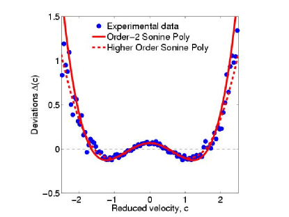
Figure 11: Experimental deviation function from Gaussian behavior, $\Delta(c)$ for $\phi=0.66$. The solid line is the Sonine polynomial $a_{2}(1/2c^{4}-3/2c^{2}+3/8)$ with one single fitting parameter: $a_{2}=0.171$. The dashed line is the higher order Sonine polynomial description of the form $\sum_{p=2}^{6}a_{p}S_{p}(c^{2})$ with the following (five fitting parameters) Sonine coefficients; $a_{2}=0.1578$, $a_{3}=-0.0656$, $a_{4}=0.1934$, $a_{5}=-0.1637$ and $a_{6}=0.0832$.

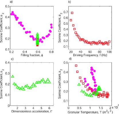
Figure 12: Experimentally determined order-two Sonine coefficient $a_{2}$ as a function of (a) filling fraction ($\bullet$), (b) driving frequency ($\square$), (c) dimensionless acceleration ($\triangle$) and (d) granular temperature. The filling fraction is kept constant at $\phi=0.59$ while exploring the dependence of $a_{2}$ on $f$ and $\Gamma$.

To check the validity of this assumption of the Kinetic Theory, we shall follow a procedure analogous to that employed in the numerical study of Ref. Moon et al. (2001). We calculate the deviation, $\Delta(c)$, of the experimental velocity distributions, $P(c)$, from the equilibrium Maxwell-Boltzmann, $f_{MB}$, such that,

$$P(c)=f_{MB}\left(1+\Delta(c)\right),$$ (19)

where $f_{MB}$ is given by Eqn. (10). By comparing Eqn. (19) to Eqn. (9) for the theoretical case of inelastic particles under a stochastic thermostat, we expect that

$$P(c)=f_{MB}(1+a_{2}S_{2}(c^{2})),$$ (20)

such that the experimental deviations from equilibrium take the form of the Sonine polynomial of order-two, $S_{2}(c^{2})$, i.e.

$$\Delta(c)=a_{2}\left(1/2c^{4}-3/2c^{2}+3/8\right),$$ (21)

where the parameter $a_{2}$ can be directly related to the kurtosis $K$ of the distribution as $a_{2}=K/3-1$. However, because of sampling noise at high $c$, we have taken $a_{2}$ as a fitting parameter rather than determining it directly from $K$, although in most cases there is little difference. Note that the fitting of the experimental data to Eqn. (20) was done over the whole range of the distribution with a relative weighting given by the corresponding probability. In Fig. 10(a–d) we plot these experimental deviation from equilibrium, $\Delta(c)$, for four representative values of filling fraction, along with the order-2 Sonine polynomial (solid curve) as given by Eqn. (21) and fitting for $a_{2}$. At low filling fractions, for example $\phi=0.34$ – Fig. 10(a) – the second order Sonine fit is approximate but unsatisfactory for small $c$ where a sharp cusped peak is present. This cusp is reminiscent of the underlying dynamics of the rough plate thermal bath as evidenced by the cusp at $c=0$ for the single particle distribution presented in Fig. 2(c) and discussed previously. On the other hand, for larger values of the filling fraction (in particular for $\phi>0.44$) the experimental data is accurately described by the second order Sonine polynomial.

To further evaluate the relevance of the Sonine polynomials to describe the experimental deviation from Maxwell-Boltzmann, in Fig. 11 we plot the experimental $\Delta(c)$ along with both the order-two ($p=2$) Sonine polynomial and the higher order Sonine expansion of the form $\sum_{p=2}^{6}a_{p}S_{p}(c^{2})$. The second order Sonine polynomial alone is responsible for the largest gain in accuracy of the corrections from MB (horizontal dashed line). The higher order Sonine expansion indeed provide a better fit but the overall improvement is only marginal (see Fig. 14.)

In Fig. 12(a) we present the dependence of the second Sonine coefficient $a_{2}$, the single fitting parameter in Eqn. (21), as a function of filling fraction. The coefficient $a_{2}$ initially decreases with increasing filling fraction up to $\phi=0.65$, after which it shows a rapid rise. We also study the dependence of $a_{2}$ on the driving frequency ($f$) and dimensionless acceleration ($\Gamma$) for a single value of the filling fraction $\phi=0.59$, which we present in Figs. 12(b) and (c), respectively. For lower values of frequency (20-40Hz) we get a monotonic drop in $a_{2}$ with increasing frequency. For $f>40Hz$, the coefficient $a_{2}$ then levels off and remains approximately constant at $a_{2}=0.171\pm 0.023$. For $\Gamma>2.0$, the coefficient $a_{2}$ remains approximately constant at $a_{2}=0.193\pm 0.029$. We have plotted these two datasets at fixed $\phi$ and varying $f$ and $\Gamma$ back in Fig. 12(a) and the behavior of $a_{2}$ is found to be consistent with the previous dataset with varying $\phi$ at fixed $(f,\Gamma)=(50Hz,4.0)$. It is interesting to note that a scatter of points is obtained if $a_{2}$ for the three previous datasets is plotted as a function of the corresponding granular temperatures. Moreover, for the data-set for varying $\phi$ the dependence is clearly not single valued, i.e. one can find two distinct values of $a_{2}$ for a single value of temperature. All this suggests that the temperature does not set $a_{2}$. Instead, $a_{2}$ is a strong function of $\phi$ and is only weakly dependent on $f$ and $\Gamma$, provided that $f>40Hz$ and $\Gamma>2$. This is in agreement with inelastic hard-sphere behavior where the only two relevant parameters are thought to be the filling fraction and the coefficient of restitution (not investigated in the present study).

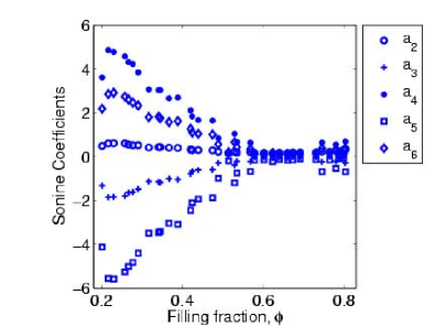
Figure 13: Dependence of higher order coefficients of the Sonine expansion ($a_{2}$ to $a_{6}$) on filling fraction.

Next, in Fig. 13 we present the dependence on filling fraction of the experimentally determined five non-zero Sonine coefficients in the sixth order expansion of $\Delta(c)\sim\sum_{p=2}^{6}a_{p}S_{p}(c^{2})$. In the theoretical analysis, the higher order terms (order 3 and above) in the Sonine polynomial expansion are typically neglected to simplify the calculations, the claim being that this results in no significant loss of accuracy. In our experimentally generated fluids the higher order Sonine coefficients assume values less than 1 for filling fractions above $\phi=0.5$. From this it is clear that it is unnecessary to consider orders higher than two for intermediate and high filling fractions. For $\phi<0.5$, however, they are significant and the finite values of $a_{3}$,…, $a_{6}$ are required to fit the increasingly larger regions of stretching exponential tails which become progressively more wider and propagate towards smaller velocities. As we mentioned in the discussion of Fig. 9(a) in the previous Sec., when the filling fraction decreases, the dynamics of the layer starts resembling that of the underlying thermal bath set by the rough plate. There the distribution, at low $c$ becomes increasingly more like a stretched exponential throughout the full $c$ range, rather than only in its tails as is the case at larger values of $\phi$. This finding is analogous to a result from Brilliantov and Pöschel Brilliantov and Poschel (2006) who found both theoretically and numerically that the magnitude of the higher-order Sonine coefficients can grow due to the an increasing impact of the overpopulated high-energy tails of the distribution function, just like in our system at low $\phi$. Their analysis was however performed as a function of the coefficient of restitution, $\epsilon$, rather than filling fraction. In their study a single second order Sonine polynomial becomes insufficient to represent the deviation from Gaussian at low values of $\epsilon$. Moreover, they worked on the Homogeneous Cooling State (HCS), but they suggest that their results should also apply to granular gases with a thermostat, like in our case. A more direct comparison with this theoretical analysis is open to further investigation.

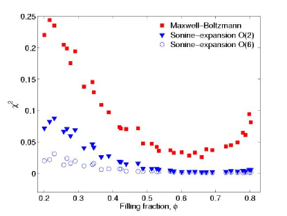
Figure 14: Deviations (quantified by $\chi^{2}$), as a function of filling fraction, of the experimental velocity distributions from Maxwell-Boltzmann distribution ($\square$), from the velocity distribution function with a order-two Sonine polynomial correction ($\triangledown$) and from the velocity distribution function with a order-six Sonine polynomial expansion correction ($\circ$) .

We stress that a finite value of the higher order coefficients does not necessarily imply a large correction to the deviations $\Delta(c)$. To explore further this point we now quantify the deviations of our experimental velocity distribution from all the three models we have considered: 1) the equilibrium Maxwell-Boltzmann distribution, 2) the velocity distribution function with order-2 Sonine polynomial expansion and, 3) the velocity distribution function with higher order Sonine polynomial terms. In Fig. 14 we plot these deviation of experiments from the models as quantified by $\chi^{2}=\sum_{i=1}^{N}(P(c_{i})_{exp}-P(c_{i})_{model})^{2}$, for the full range of filling fractions. We clearly see significant deviation of the experimental data from Maxwell-Boltzmann distribution for all $\phi$, whereas the velocity distributions with the order-2 Sonine polynomial term shows a considerably better agreement with the experimental data across the whole range of $\phi$. Even though the higher order Sonine polynomial expansion characterizes the experimental data more closely, these higher order contributions are modest compared with the large gain in accuracy from the order-2 Sonine polynomial alone, and in the range of $\phi>0.44$ provide no significant improvement. Thus the order-2 description obtained by neglecting the higher order Sonine terms is a reasonably good approximation to describe the experimental data.

VII Conclusion

In conclusion, we have developed an experimental model system for a quasi-2D granular layer, under homogeneous stochastic driving. Our experimental technique has allowed us to randomly thermalize a granular fluid over a wide range of filling fractions. Our study was centered on the dynamics of the system, in particular the statistics of velocities. The temperature of the experimental granular fluid could be adjusted by varying the system’s control parameters, namely the filling fraction, the frequency and acceleration of the driving and the gap height, with no significant change in the nature of the velocity probability distribution functions. We have found an excellent collapse of the distribution functions if the particle velocities are scaled by a characteristic velocity $v_{o}$ (the standard deviation of the distributions).

However, the obtained distribution are non-Gaussian. We have analyzed the deviations from Gaussian behavior in two distinct regimes. Firstly, we looked at the shape of the distribution tails which scaled as stretched exponentials with exponent $-3/2$. Secondly, we have performed an expansion method that highlights the deviations from a Gaussian at low velocities (near $c=0$) and found them to be Sonine-like, i.e. polynomial of order four with fixed coefficients. This way we have determined the validity of some important assumptions in the Kinetic Theory of randomly driven fluids. It is surprising that this formalism seems applicable at filling fractions as high as $\phi=0.80$, whereas Kinetic Theory is usually thought to breakdown at much lower values of $\phi$. Finally, we have looked at Sonine polynomial expansion with higher order terms and concluded that it is sufficient to retain only the leading order (first non-vanishing) term to maintain reasonable accuracy of the polynomial expansion. Therefore, we can accurately characterize the single particle velocity distribution function by introducing a single extra coefficient $a_{2}$, in addition to the 0th, 1st and 2nd moments used for fluids at equilibrium. The coefficient $a_{2}$ has universal character in the sense that it is a strong function of filling fraction and only depends weakly on the other experimental parameters such as the driving frequency and acceleration.

Having determined the base state of our randomly driven granular fluid, we hope that an experimental system such as ours can be used further as a laboratory test bed of some basic assumptions of Kinetic Theory. In future work, it would also be of interest to investigate whether particle-particle velocity correlations Prevost et al. (2002) are present in our system but this is beyond the scope of the current investigation.

To our knowledge, this is the first time that the Sonine corrections of the central high probability regions of the velocity distributions have been measured in an experimental system, in agreement with analytical predictions. This should open way to further theoretical developments, crucial if we are to develop much desired predictive models for granular flows with practical relevance.

Appendix A Probability density functions of velocities using the bottom flat plate

In this Appendix we discuss the nature of the velocity distributions obtained using a flat bottom plate as in the system of Olafsen and Urbach Olafsen and Urbach (1999). The distributions $P(v)$ are presented in Figs. 15(a) for a wide range of filling fractions. Unlike the case of using a rough plate, here there is an enormous variation in the shape of $P(v)$. At low $\phi$ the distributions are sharply peaked near $c=0$. The value of $P(v=0)$ can differ by over a factor of 20 between low and high $\phi$. In Fig. 15(b) the distributions $P(c)$ – obtained after rescaling all velocities by the characteristic velocity $v_{o}$ given by Eqn. (17) – do not collapse onto a single curve and show considerably larger deviations from a Maxwell-Boltzmann (solid line). This distributions only attain the general form found for the rough case at filling fractions larger than $\phi>0.6$ and this is in agreement with the point at which the granular temperature of both cases coincide – Fig. 4. For this high values of $\phi$, both in the rough and flat cases, the contribution to the thermalization is more important from the large number inter-particle collisions rather than the underlying thermostat. Hence we expect the analysis we have performed throughout this paper to be applicable to the flat case, for $\phi>0.6$, but not below this point.

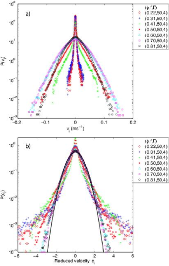
Figure 15: PDF of velocities for an experimental cell where both top and bottom plates were optically flat. (a) $P(v)$ (b) $P(c)$, in which all velocities for each distribution were normalized by its standard deviation. The solid line is a Maxwell-Boltzmann distribution with unit standard deviation. Data for a range of parameters: $\phi$, $f$ and $\Gamma$ (see legends for specific values).

In addition to the discussion on the granular temperature of Sec. V, these results present further evidence for the significant advantage of using a rough bottom plate to generate the thermostat to heat the granular fluid in a way that may be directly compared to theoretical work on inelastic hard-spheres driven by a stochastic thermostat.

This work is funded by The National Science Foundation, Math, Physical Sciences Department of Materials Research under the Faculty Early Career Development (CAREER) Program (DMR-0134837). PMR was partially funded by the Portuguese Ministry of Science and Technology under the POCTI program and the MECHPLANT NEST-Adventure program of the European Union.

References

- Jaeger et al. (1996) H. Jaeger, S. R. Nagel, and R. P. Behringer, Rev. Mod. Phys. 68, 1259 (1996).
- Kadanoff (1999) L. Kadanoff, Rev. Mod. Phys. 71, 435 (1999).
- Melo et al. (1994) F. Melo, P. Umbanhowar, and H. L. Swinney, Phys. Rev. Lett. 72, 172 (1994).
- Miller et al. (1996) B. Miller, C. O’Hern, and R. P. Behringer, Phys. Rev. Lett. 77, 3110 (1996).
- Reis et al. (2006a) P. M. Reis, R. A. Ingale, and M. D. Shattuck, Phys. Rev. Lett. 96, 258001 (2006a).
- Reis et al. (2006b) P. Reis, R. Ingale, and M. Shattuck (2006b), submitted to Phys. Rev. Lett. , preprint: cond-mat/0610489.
- Savage and Jeffery (1981) S. Savage and D. Jeffery, J. Fluid Mech 110, 255 (1981).
- Lun et al. (1983) C. Lun, S. Savage, D. Jeffery, and N. Chepurniy, J. Fluid. Mech. 140, 223 (1983).
- Jenkins and Richman (1985a) J. Jenkins and M. Richman, Arch. Ration. Mech. Anal. 87, 355 (1985a).
- Jenkins and Richman (1985b) J. Jenkins and M. Richman, Phys. Fluids 28, 3485 (1985b).
- Jenkins and Richman (1988) J. T. Jenkins and M. W. Richman, J. Fluid Mech. 192, 313 (1988).
- Lun (1991) C. K. K. Lun, J. Fluid Mech. 233, 539 (1991).
- Goldshtein and Shapiro (1995a) A. Goldshtein and M. Shapiro, J. Fluid Mech. 282, 75 (1995a).
- Sela et al. (1996) N. Sela, I. Goldhirsch, and S. H. Noskowicz, Phys. Fluids 8, 2337 (1996).
- Brey et al. (1996) J. J. Brey, F. Moreno, and J. W. Dufty, Phys. Rev. E 54, 445 (1996).
- Santos et al. (1998) A. Santos, J. M. Montanero, J. W. Dufty, and J. J. Brey, Phys. Rev. E 57, 1644 (1998).
- van Noije et al. (1998a) T. P. C. van Noije, M. H. Ernst, and R. Brito, Physica A 251, 266 (1998a).
- Garzó and Dufty (1999) V. Garzó and J. Dufty, Phys. Rev. E 60, 5706 (1999).
- Dufty and Brey (2003) J. W. Dufty and J. J. Brey, Phys. Rev. E 68, 030302(R) (2003).
- Brey and Ruiz-Montero (2004) J. J. Brey and M. J. Ruiz-Montero, Phys. Rev. E 70, 051301 (2004).
- Dufty et al. (2004) J. W. Dufty, A. Baskaran, and L. Zogaib, Phys. Rev. E 69, 051301 (2004).
- Kumaran (2005) V. Kumaran, Phys. Rev. Lett. 95, 108001 (2005).
- Brey and Dufty (2005) J. J. Brey and J. W. Dufty, Phys. Rev. E 72, 011303 (2005).
- Lutsko (2006) J. F. Lutsko, Phys. Rev. E 73, 021302 (2006).
- Losert et al. (1999) W. Losert, D. G. W. Cooper, , J. Delour, A. Kudrolli, and J. P. Gollub, Chaos 9, 682 (1999).
- Olafsen and Urbach (1999) J. S. Olafsen and J. S. Urbach, Phys. Rev. E 60, R2468 (1999).
- Rouyer and Menon (2000) F. Rouyer and N. Menon, Phys. Rev. Lett. 85, 3676 (2000).
- Blair and Kudrolli (2001) D. L. Blair and A. Kudrolli, Phys. Rev. E 64, 050301(R) (2001).
- Prevost et al. (2002) A. Prevost, D. A. Egolf, and J. S. Urbach, Phys. Rev. Lett. 89, 084301 (2002).
- Aranson and Olafsen (2002) I. S. Aranson and J. S. Olafsen, Phys. Rev. E 66, 061302 (2002).
- Blair and Kudrolli (2003) D. L. Blair and A. Kudrolli, Phys. Rev. E 67, 041301 (2003).
- Moon et al. (2001) S. J. Moon, M. D. Shattuck, and J. B. Swift, Phys. Rev. E 64, 031303 (2001).
- van Noije and Ernst (1998) T. van Noije and M. Ernst, Granular Matter 1, 57 (1998).
- Williams and MacKintosh (1996) D. R. M. Williams and F. C. MacKintosh, Phys. Rev. E 54, R9 (1996).
- van Noije et al. (1999) T. P. C. van Noije, M. H. Ernst, E. Trizac, and I. Pagonabarraga, Phys. Rev. E 59, 4326 (1999).
- Montanero and Santos (2000) J. Montanero and A. Santos, Granular Matter 2, 53 (2000).
- Brilliantov and Poschel (2006) N. V. Brilliantov and T. Poschel, Europhys. Lett. 74, 424 (2006).
- Pöschel et al. (2006) T. Pöschel, N. V. Brilliantov, and A. Formella, Phys. Rev. E 74, 041302 (2006).
- van Noije et al. (1998b) T. van Noije, M. Ernst, and R. Brito, Physica A 251, 266 (1998b).
- Goldshtein and Shapiro (1995b) I. Goldshtein and M. Shapiro, J. Fluid Mech 282, 75 (1995b).
- Alder and Wainwright (1962) B. Alder and T. Wainwright, Phys. Rev. E 127, 359 (1962).
- Mitus et al. (1997) A. C. Mitus, H. Weber, and D. Marx, Phys. Rev. E 55, 6855 (1997).
- van Zon et al. (2004) J. S. van Zon, J. Kreft, D. I. Goldman, D. Miracle, J. B. Swift, and H. L. Swinney, Phys. Rev. E 70, 040301(R) (2004).
- Barrat and Trizac (2003) A. Barrat and E. Trizac, Euro. Phys. J. E 11, 99 (2003).
- Barrat et al. (2005) A. Barrat, E. Trizac, and M. H. Ernst, J. of Phys: Condens. Matt. 17, 2005 (2005).