Resonantly-paired fermionic superfluids

Abstract

We present a theory of a degenerate atomic Fermi gas, interacting through a narrow Feshbach resonance, whose position and therefore strength can be tuned experimentally, as demonstrated recently in ultracold trapped atomic gases. The distinguishing feature of the theory is that its accuracy is controlled by a dimensionless parameter proportional to the ratio of the width of the resonance to Fermi energy. The theory is therefore quantitatively accurate for a narrow Feshbach resonance. In the case of a narrow $s$-wave resonance, our analysis leads to a quantitative description of the crossover between a weakly-paired BCS superconductor of overlapping Cooper pairs and a strongly-paired molecular Bose-Einstein condensate of diatomic molecules. In the case of pairing via a $p$-wave resonance, that we show is always narrow for a sufficiently low density, we predict a detuning-temperature phase diagram, that in the course of a BCS-BEC crossover can exhibit a host of thermodynamically-distinct phases separated by quantum and classical phase transitions. For an intermediate strength of the dipolar anisotropy, the system exhibits a $p_{x}+ip_{y}$ paired superfluidity that undergoes a topological phase transition between a weakly-coupled gapless ground state at large positive detuning and a strongly-paired fully-gapped molecular superfluid for a negative detuning. In two dimensions the former state is characterized by a Pfaffian ground state exhibiting topological order and non-Abelian vortex excitations familiar from fractional quantum Hall systems.

I Introduction

I.1 Weakly- and strongly-paired fermionic superfluids

Paired superfluidity in Fermi systems is a rich subject with a long history dating back to the discovery of superconductivity (charged superfluidity) in mercury by Kamerlingh Onnes in 1911. Despite considerable progress on the phenomenological level and many experimental realizations in other metals that followed, a detailed microscopic explanation of superconductivity had to await seminal breakthrough by Bardeen, Cooper and Schrieffer (BCS) (for the history of the subject see, for example, Ref. Schrieffer (1989) and references therein). They discovered that in a degenerate, finite density system, an arbitrarily weak fermion attraction destabilizes the Fermi sea (primarily in a narrow shell around the Fermi energy) to a coherent state of strongly overlaping “Cooper pairs” composed of weakly correlated time-reversed pairs of fermions.

In contrast, superfluidity in systems (e.g., liquid ⁴He), where constituent fermions (neutrons, protons, electrons) are strongly bound into a nearly point-like bosonic atom, was readily qualitatively identified with the strongly interacting liquid limit of the Bose-Einstein condensation of composite bosonic ⁴He atoms (for a review, see for example Ref. Khalatnikov (2000)).

While such weakly- and strongly-paired fermionic $s$-wave superfluids were well understood by early 1960’s, the relation between them and a quantitative treatment of the latter remained unclear until Eagles’s Eagles (1969) and later Leggett’s Leggett (1980), and Nozières and Schmitt-Rink’s Nozières and Schmitt-Rink (1985) seminal works. Working with the mean-field BCS model, that is quantitatively valid only for a weak attraction and high density (a superconducting gap much smaller than the Fermi energy), they boldly applied the model outside its quantitative range of validity Levinsen and Gurarie (2006) to fermions with an arbitrarily strong attraction. Effectively treating the BCS state as a variational ground state, such approach connected in a concrete mean-field model the two types of $s$-wave paired superfluids, explicitly demonstrating that they are two extreme regimes of the same phenomenon, connected by a smooth (analytic) crossover as the strength of attractive interaction is varied from weak to strong. This lack of qualitative distinction between a “metallic” (BCS) and “molecular” (BEC) $s$-wave superfluids, both of which are characterized by a complex scalar (bosonic) order parameter $\Psi$, was also anticipated much earlier based on symmetry grounds by the Ginzburg-Landau theory Schrieffer (1989).

Nevertheless, the two types of superfluids regimes exhibit drastically (quantitatively com (a)) distinct phenomenologies Nozières and Schmitt-Rink (1985); Sá de Melo et al. (1993). While in a weakly-paired BCS superconductor the transition temperature $T_{c}$ nearly coincides with the Cooper-pair binding (dissociation) energy, that is exponentially small in the pairing potential, in the strongly-paired BEC superfluid $T_{c}$ is determined by the density, set by the Fermi temperature, and is nearly independent of the attractive interaction between fermions. In such strongly coupled systems the binding energy, setting the temperature scale $T_{*}$ above which the composite boson dissociates into its constituent fermions (e.g., of order eV in ⁴He) can therefore be orders of magnitude larger than the actually condensation temperature $T_{c}\ll T_{*}$. This large separation between $T_{c}$ and $T_{*}$ is reminiscent of the phenomenology observed in the high-temperature superconductors (with the range $T_{c}<T<T_{*}$ referred to as the “pseudo-gap” regime), rekindling interest in the BCS-BEC crossover in the mid-90’s Sá de Melo et al. (1993) and more recently Chen et al. (2005).

With a discovery of novel superconducting materials (e.g., high-T_c’s, heavy fermion compounds), and superfluids (³He), that are believed to exhibit finite angular momentum pairing, the nature of strongly- and weakly-paired superfluids has received even more attention. It was soon appreciated Volovik (1992); Read and Green (2000); Volovik (2003) that, in contrast to the $s$-wave case, strongly and weakly paired states at a finite angular momentum are qualitatively distinct. This is most vividly illustrated in three dimensions, where for weak attraction a two-particle bound state is absent, the pairing is stabilized by a Fermi surface and therefore necessarily exhibits nodes and gapless excitations in the finite angular momentum paired state. In contrast, for strong attraction a two-particle bound state appears, thereby exhibiting a fully-gapped superfluidity with concomitant drastically distinct low temperature thermodynamics. Other, more subtle topological distinctions, akin to quantum Hall states, between the two types of paired grounds states also exist and have been investigated Read and Green (2000); Volovik (1992). Consequently, these qualitative distinctions require a genuine quantum phase transition (rather than an analytic crossover, as in the case of $s$-wave superfluid) to separate the weakly and strongly-paired states. This transition should be accessible if the pairing strength were experimentally tunable.

I.2 Paired superfluidity via a Feshbach resonance

The interest in paired superfluidity was recently revived by the experimental success in producing degenerate (temperature well below Fermi energy) trapped atomic Fermi gases of ⁶Li and ⁴⁰K  DeMarco and Jin (1999); Strecker et al. (2003); Regal et al. (2004); Zwierlein et al. (2004). A remarkable new experimental ingredient is that the atomic two-body interactions in these systems can be tuned by an external magnetic field to be dominated by the so-called Feshbach resonant (FR) Feshbach (1958); Tiesinga et al. (1993) scattering through an intermediate molecular (virtual or real bound) state.

As depicted in Fig. 1, such tunable Feshbach resonance Timmermans et al. (1999) arises in a system where the interaction potential between two atoms depends on their total electron spin state, admitting a bound state in one spin channel (usually referred to as the “closed channel”, typically an approximate electron spin-singlet). The interaction in the second sim “open” channel (usually electron spin triplet, that is too shallow to admit a bound state) is then dominated by a scattering through this closed channel resonance com (b). Since the two channels, coupled by the hyperfine interaction, generically have distinct magnetic moments, their relative energies (the position of the Feshbach resonance) and therefore the open-channel atomic interaction can be tuned via an external magnetic field through the Zeeman splitting, as depicted in Fig. 1.

Figure 1: Interactions between the atoms generically depends on their mutual spin state. This figure depicts two potentials corresponding to two spin states of the pairs of atoms. One of them (usually referred to as an “open channel”) is too weak to support a bound state, while the other (a “closed channel”) supports a bound state, but is energetically unfavorable at large distances. The closed channel potential can be moved vertically with respect to the open channel potential via the Zeeman effect, by changing an external magnetic field.

In the dilute, two-body limit the low-energy $s$-wave Feshbach resonant scattering is characterized by an $s$-wave scattering length, that, as illustrated in Fig.2, is observed to behave according to Inouye et al. (1998); Moerdijk et al. (1995)

$$a(H)=a_{bg}\left(1-\frac{H_{w}}{H-H_{0}}\right),$$ (1)

diverging as the magnetic field passes through a (system-dependent) field $H_{0}$, corresponding to a tuning of the resonance through zero energy. (Analogously, a $p$-wave resonance is characterized by a scattering volume $v(H)$, as discussed in detail in Sec. II.2). In above, the experimentally measurable parameters $a_{bg}$ and $H_{w}$ are, respectively, the background (far off-resonance) scattering length and the so-called (somewhat colloquially; see  com (c)) magnetic “resonance width”.

An $s$-wave Feshbach resonance is also characterized by an additional length scale, the so-called effective range $r_{0}$, and a corresponding energy scale

$$\Gamma_{0}=\frac{4\hbar^{2}}{mr_{0}^{2}},$$ (2)

that only weakly depend on $H$. This important scale measures the intrinsic energy width of the two-body resonance and is related to the measured magnetic-field width $H_{w}$ via

$$\Gamma_{0}\approx 4m\mu_{B}^{2}a_{bg}^{2}H_{w}^{2}/\hbar^{2},$$ (3)

with $\mu_{B}$ the Bohr magneton. $\Gamma_{0}$ sets an energy crossover scale between two regimes of (low- and intermediate-energy) behavior of two-atom $s$-wave scattering amplitude.

A key observation is that, independent of the nature of the complicated atomic interaction leading to a Feshbach resonance, its resonant physics outside of the short microscopic (molecular size of the closed-channel) scale can be correctly captured by a pseudo-potential with an identical low-energy two-body scattering amplitude, that, for example, can be modeled by a far simpler potential exhibiting a minimum separated by a large barrier, as illustrated in Fig. 5. The large barrier suppresses the decay rate of the molecular quasi-bound state inside the well, guaranteeing its long lifetime even when its energy is tuned above the bottom of the continuum of states.

Although such potential scattering, Fig. 5 is microscopically quite distinct from the Feshbach resonance, Fig. 1, this distinction only appears at high energies. As we will see, the low energy physics of a shallow resonance is controlled by a nearly universal scattering amplitude, that depends only weakly on the microscopic origin of the resonance. Loosely speaking, for a large barrier of a potential scattering depicted on Fig. 5 one can associate (quasi-) bound state inside the well with the closed molecular channel, the outside scattering states with the open channel, and the barrier height with the hyperfine interactions-driven hybridization of the open and closed channels of the Feshbach resonant system. The appropriate theoretical model was first suggested in Ref. Timmermans et al. (1999), and in turn exhibits two-body physics identical to that of the famous Fano-Anderson model Fano (1961) of a single level inside a continuum (see Appendix B).

A proximity to a Feshbach resonance allows a high tunability (possible even in “real” time) of attractive atomic interactions in these Feshbach-resonant systems, through a resonant control of the $s$-wave scattering length $a(H)$, Eq. (1) via a magnetic field. As we will discuss in Sec. VII, a $p$-wave Feshbach resonance similarly permits studies of $p$-wave interacting systems with the interaction tunable via a resonant behavior of the scattering volume $v(H)$. This thus enables studies of paired superfluids across the full crossover between the BCS regime of weakly-paired, strongly overlapping Cooper pairs, and the BEC regime of tightly bound (closed-channel), weakly interacting diatomic molecules. More broadly, it allows access to interacting atomic many-body systems in previously unavailable highly coherent and even nonequilibrium regimes Donley et al. (2001); Barankov and Levitov (2004); Andreev et al. (2004), unimaginable in more traditional solid state systems.

Figure 2: A schematic of a typical, experimentally observed behavior of an $s$-wave scattering length $a(H)$ as a function of magnetic field $H$ in a vicinity of a Feshbach resonance.

I.3 Narrow vs wide resonances and model’s validity

An atomic gas at a finite density $n$ (of interest to us here) provides an additional length, $n^{-1/3}\sim k_{F}^{-1}$ and corresponding energy, $\epsilon_{F}=\hbar^{2}k_{F}^{2}/2m$ scales. For the $s$-wave resonance, these scales, when combined with the length $r_{0}$ or the resonance width $\Gamma_{0}$, respectively, allow us to define an $s$-wave dimensionless parameter (with numerical factor chosen for later convenience)

$$\gamma_{s}=\frac{\sqrt{8}}{\pi}\sqrt{\Gamma_{0}\over\epsilon_{F}}=\frac{8}{\pi}{\hbar\over k_{F}|r_{0}|},$$ (4)

that measures the width of the resonance or equivalently the strength of the Feshbach resonance coupling (hybridization of an atom-pair with a molecule) relative to Fermi energy. For a $p$-wave (and higher angular momentum) resonance a similar dimensionless parameter can be defined (see below). The key resonance-width parameter $\gamma$ com (c) naturally allows a distinction between two types of finite density Feshbach-resonant behaviors, a narrow ($\gamma\ll 1$) and broad ($\gamma\gg 1$). Physically, these are distinguished by how the width $\Gamma_{0}$ compares with a typical atomic kinetic energy $\epsilon_{F}$. Equivalently, they are contrasted by whether upon growth near the resonance, the scattering length $a(H)$ first reaches the effective range $|r_{0}|$ (broad resonance) or the atom spacing $\ell$ (narrow resonance).

Systems exhibiting a narrow resonant pairing are extremely attractive from the theoretical point of view. As was first emphasized in Ref. Andreev et al., 2004 and detailed in this paper, such systems can be accurately modeled by a simple two-channel Hamiltonian characterized by the small dimensionless parameter $\gamma$, that remains small (corresponding to long-lived molecules) throughout the BCS-BEC crossover. Hence, while nontrivial and strongly interacting, narrow Feshbach resonant systems allow a quantitative analytical description, detailed below, that can be made arbitrarily accurate (exact in the zero resonance width limit), with corrections controlled by powers of the small dimensionless parameter $\gamma$, computable through a systematic perturbation theory in $\gamma$. The ability to treat narrowly resonant systems perturbatively physically stems from the fact that such an interaction, although arbitrarily strong at a particular energy, is confined only to a narrow energy window around a resonant energy.

As we will show in this paper Andreev et al. (2004), such narrow resonant systems exhibit a following simple picture of a pairing superfluid across the BCS-BEC crossover, illustrated in Fig. 3. For a Feshbach resonance tuned to a positive (detuning) energy the closed-channel state is a resonance Res , that generically leads to a negative scattering length and an effective attraction between two atoms in the open-channel. For detuning larger than twice the Fermi energy, most of the atoms are in the open-channel, forming a weakly BCS-paired Fermi sea, with exponentially small molecular density, induced by a weak Feshbach resonant (2-)atom-molecule coupling (hybridization). The BCS-BEC crossover initiates as the detuning is lowered below $2\epsilon_{F}$, where a finite density of atoms binds into Bose-condensed (at $T=0$) closed-channel quasi-molecules, stabilized by the Pauli principle. The formed molecular (closed-channel) superfluid coexists with the strongly-coupled BCS superfluid of (open-channel) Cooper pairs, that, while symmetry-identical and hybridized with it by the Feshbach resonant coupling is physically distinct from it. This is made particularly vivid in highly anisotropic, one dimensional traps, where the two distinct (molecular and Cooper-pair) superfluids can actually decouple due to quantum fluctuations suppressing the Feshbach coupling at low energies Sheehy and Radzihovsky (2006a). The crossover to BEC superfluid terminates around zero detuning, where conversion of open-channel atoms (forming Cooper pairs) into closed-channel molecules is nearly complete. In the asymptotic regime of a negative detuning a true bound state appears in the closed-channel, leading to a positive scattering length and a two-body repulsion in the open-channel. In between, as the position of the Feshbach resonance is tuned through zero energy, the system is taken through (what would at zero density be) a strong unitary scattering limit, corresponding to a divergent scattering length, that is nevertheless quantitatively accessible in a narrow resonance limit, where $\gamma_{s}\sim 1/(k_{F}r_{0})$ plays the role of a small parameter.

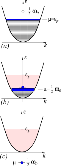
Figure 3: An illustration of the BCS-BEC crossover in the limit of a narrow Feshbach resonance width, $\gamma_{s}\ll 1$. The evolution with detuning $\omega_{0}$ is illustrated, with (a) the BCS regime of $\omega_{0}>2\epsilon_{F}$, where particles are predominantly open-channel atoms forming a Cooper-paired Fermi sea, (b) the crossover regime of $0<\omega_{0}<2\epsilon_{F}$, where a fraction of atoms between $\omega_{0}$ and $\epsilon_{F}$ have converted into a BEC of bosonic (closed-channel) molecules, with the rest forming a Cooper-paired Fermi sea at a chemical potential $\mu$, and (c) the BEC regime of $\omega_{0}<0$, where (to order $\gamma_{s}\ll 1$) only Bose-condensed molecules are present.

This contrasts strongly with systems interacting via a featureless attractive (e.g., short-range two-body) potential, where due to a lack of a large potential barrier (see Fig. 12) no well-defined (long-lived) resonant state exists at positive energy and a parameter $\gamma_{s}$ (proportional to the inverse of effective range $r_{0}$) is effectively infinite. For such broad-resonance systems, a gas parameter $n^{1/3}\left|a(H)\right|$ is the only dimensionless parameter. Although for a dilute gas ($n^{1/3}a_{bg}\ll 1$) a controlled, perturbative analysis (in a gas parameter) of such systems is possible away from the resonance, where $n^{1/3}\left|a(H)\right|\ll 1$, a description of the gas (no matter how dilute), sufficiently close to the resonance, such that $n^{1/3}|a(H)|>1$ is quantitatively intractable in broad-resonance systems Eps . This important distinction between the narrow and broad Feshbach resonances and corresponding perturbatively-(in)accessible regions in the $k_{F}$  -  $a^{-1}$ plane around a Feshbach resonance are illustrated in Fig. 4.

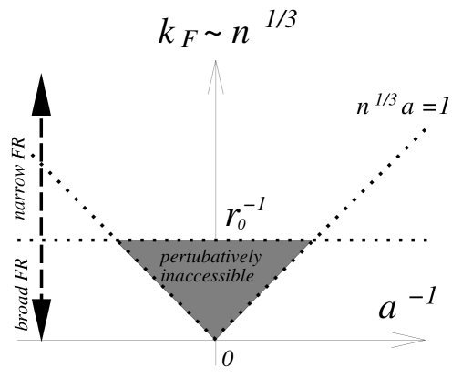
Figure 4: An illustration of perturbatively accessible and inaccessible (grey) regions in the inverse particle spacing vs inverse scattering length, $n^{1/3}$–$a^{-1}$ plane around a Feshbach resonace, where $a$ diverges. Note that outside the grey region, even for a broad Feshbach resonance there is a small parameter that is either the gas parameter or Feshbach resonance coupling, or both, and hence the system can be analyzed perturbative.

.

Nevertheless, because of their deceiving simplicity and experimental motivation (most current experimental systems are broad), these broad-resonance systems (exhibiting no long-lived positive energy resonance Res ) were a focus of the aforementioned earlier studies Eagles (1969); Leggett (1980); Nozières and Schmitt-Rink (1985); Sá de Melo et al. (1993) that provided a valuable qualitative elucidation of the BCS-BEC crossover into the strongly-paired BEC superfluids. However, (recent refinements, employing enlightening but uncontrolled approximations notwithstanding Timmermans et al. (1999); Holland et al. (2001); Ohashi and Griffin (2002); Chen et al. (2005)) these embellished mean-field descriptions are quantitatively untrustworthy outside of the BCS regime, where weak interaction (relative to the Fermi energy) provides a small parameter justifying a mean-field treatment – and outside of the BEC regime where, although mean-field techniques break down, a treatment perturbative in $n^{1/3}|a|\ll 1$ is still possible Levinsen and Gurarie (2006). The inability to quantitatively treat the crossover regime for generic (non-resonant) interactions is not an uncommon situation in physics, where quantitative analysis of the intermediate coupling regime requires an exact or numerical solution Bulgac et al. (2006). By integrating out the virtual molecular state, systems interacting through a broad (large $\gamma$) resonance can be reduced to a nonresonant two-body interaction of effectively infinite $\gamma$, and are therefore, not surprisingly, also do not allow a quantitatively accurate perturbative analysis outside of the BCS weak-coupling regime Eps .

The study of a fermionic gas interacting via a broad resonance reveals the following results. If $a<0$ (the interactions are attractive but too weak to support a bound state) and $n^{1/3}|a|\ll 1$, such a superfluid is the standard BCS superconductor described accurately by the mean-field BCS theory. If $a>0$ (the interactions are attractive and strong enough to support a bound state) and $n^{1/3}a\ll 1$, the fermions pair up to form molecular bosons which then Bose condense. The resulting molecular Bose condensate can be studied using $n^{1/3}a$ as a small parameter. In particular, in a very interesting regime where $a\gg|r_{0}|$ (even though $a\ll n^{-1/3}$) the scattering length of the bosons becomes approximately $a_{b}\approx 0.6a$ Petrov et al. (2005), and the Bose condensate behaves as a weakly interacting Bose gas with that scattering length Lifshitz and Pitaevskii (1980), as shown in Ref. Levinsen and Gurarie (2006). Finally, when $|a|n^{1/3}\gg 1$, the mean-field theory breaks down, the superfluid is said to be in the BCS-BEC crossover regime, and its properties so far could for the most part be only studied numerically, although with some encouraging recent analytical progress in this direction Eps . Much effort is especially concentrated on understanding the $|a|n^{1/3}\rightarrow\infty$ unitary regime Bulgac et al. (2006) (so called because the fermion scattering proceeds in the unitary limit and the behavior of the superfluid becomes universal, independent of anything but its density).

In this paper we concentrate solely on resonantly-paired superfluids with narrow resonances, amenable to an accurate treatment by mean-field theory regardless of the scattering length $a$. The identification of a small parameter Andreev et al. (2004); Eps , allowing a quantitative treatment of the BCS-BEC crossover in resonantly-paired superfluids in itself constitutes a considerable theoretical progress. In practice most $s$-wave Feshbach resonances studied up to now correspond to $\gamma_{s}\simeq 10$, which is consistent with the general consensus in the literature that they are wide. Yet one notable exception is the very narrow resonance discussed in Ref. Strecker et al. (2003) where we estimate $\gamma_{s}\simeq 0.1$; for a more detailed discussion of this, see Sec. IX.

Even more importantly is the observation that the perturbative parameter $\gamma$ is density- (Fermi energy, $\epsilon_{F}$) dependent, scaling as $\gamma_{s}\sim 1/\sqrt{\epsilon_{F}}$, $\gamma_{p}\sim\sqrt{\epsilon_{F}}$ for an $s$-wave and $p$-wave Feshbach resonant pairing respectively. Hence, even resonances that are classified as broad for currently achievable densities can in principle be made narrow by working at higher atomic densities.

Figure 5: A potential with a low-energy bound state whose energy is shown by a dashed line. If the potential is modified to make it more shallow, the bound state disappears altogether, replaced by a virtual bound state. If the potential is made even more shallow, a resonance - a state with positive energy and finite lifetime - appears.

I.4 Finite angular momentum resonant pairing: $p$-wave superfluidity

We also study a $p$-wave paired superfluidity driven by a $p$-wave Feshbach resonance, where the molecular (closed-channel) level is in the angular momentum $\ell=1$ state. While in degenerate atomic gases a $p$-wave superfluidity has not yet been experimentally demonstrated, the existence of a $p$-wave Feshbach resonance at a two-body level has been studied in exquisite experiments in ⁴⁰K and ⁶Li  Ticknor et al. (2004); Schunck et al. (2005). Recently, these have duly attracted considerable theoretical attention Ho and Diener (2005); Ohashi (2005); Botelho and Sá de Melo (2005); Gurarie et al. (2005); Cheng and Yip (2005).

One might worry that at low energies, because of the centrifugal barrier, $s$-wave scattering will always dominate over a finite angular momentum pairing. However, this is easily avoided by working with a single fermion species, in which the Pauli exclusion principle prevents identical fermionic atoms from scattering via an $s$-wave channel, with a $p$-wave scattering therefore dominating com (d). Being the lowest angular momentum channel in a single-species fermionic gas not forbidden by the Pauli exclusion principle, a $p$-wave interaction is furthermore special in that, at low energies it strongly dominates over the higher (than $\ell=1$) angular momentum channels.

There is a large number of features special to $p$-wave resonant superfluids that make them extremely interesting, far more so than their $s$-wave cousins. Firstly, as we will show in Sec. II.2 and V.2.2, $p$-wave (and higher angular-momentum) resonances are naturally narrow, since at finite density a dimensionless measure of their width scales as $\gamma_{p}\equiv\gamma_{1}\sim\epsilon_{F}^{1/2}$ ($\gamma_{\ell}\sim\epsilon_{F}^{\ell-1/2}$ in the $\ell$ angular momentum channel), that in contrast to the $s$-wave case can be made arbitrarily narrow by simply working at sufficiently low densities (small $\epsilon_{F}$). Consequently, a narrow $p$-wave Feshbach-resonant superfluid, that can be described arbitrarily accurately c2l at sufficiently low densities for any value of detuning, is, in principle, experimentally realizable.

Secondly, superfluids paired at a finite angular-momentum are characterized by richer order parameters (as exemplified by a $p$-wave paired ³He, heavy-fermion compounds, and $d$-wave high-T_c superconductors) corresponding to different projections of a finite angular momentum and distinct symmetries, and therefore admit sharp quantum (and classical) phase transitions between qualitatively distinct $\ell$-wave paired superfluid ground states. In fact, as we will show, even purely topological (non-symmetry changing) quantum phase transitions at a critical value of detuning are possible Klinkhamer and Volovik (2004); Read and Green (2000); Gurarie et al. (2005); Botelho and Sá de Melo (2005). This contrasts qualitatively with a smooth (analytic) BCS-BEC crossover (barring an “accidental” first-order transition), guaranteed by the aforementioned absence of a qualitative difference between BCS and BEC paired superfluidity.

Thirdly, some of the $p$-wave (and higher angular momentum) paired states are isomorphic to the highly nontrivial fractional quantum Hall effect ground states (e.g., the Pfaffian Moore-Read state) that have been demonstrated to display a topological order and excitations (vortices) that exhibit non-Abelian statistics Read and Green (2000). Since these features are necessary ingredients for topological quantum computing Kitaev (2003), a resonant $p$-wave paired atomic superfluid is an exciting new candidate Gurarie et al. (2005) for this approach to fault-tolerant quantum computation.

Finally, a strong connection to unconventional finite angular momentum superconductors in solid-state context, most notably the high-temperature superconductors provides an additional motivation for our studies.

I.5 Outline

This paper, while quite didactic, presents considerable elaboration and details on our results reported in two recent Letters Andreev et al. (2004); Gurarie et al. (2005). The rest of it is organized as follows. We conclude this Introduction section with a summary of our main experimentally relevant results. In Sec. II we present general, model-independent features of a low and intermediate energy $s$-wave and $p$-wave scattering, with and without low energy resonances present. In Sec. III we discuss general features of the microscopic models of scattering, tying various forms of scattering amplitudes discussed in Sec. II to concrete scattering potentials. We introduce one- and two-channel models of $s$-wave and $p$-wave Feshbach resonances Timmermans et al. (1999); Holland et al. (2001) in Sec. IV and Sec. V, compute exactly the corresponding two-body scattering amplitudes measured in experiments, and use them to fix the parameters of the two corresponding model Hamiltonians. These models then by construction reproduce exactly the experimentally-measured two-body physics. In the Sec. VI we use the resulting $s$-wave Hamiltonian to study the $T=0$ narrow resonance BCS-BEC crossover in an $s$-wave resonantly-paired superfluid, and compute as a function of detuning the molecular condensate fraction, the atomic (single-particle) spectrum, the 0th-sound velocity, and the condensate depletion. In the Sec. VI.2.4 contained within the Sec. VI, we extend these results to a finite temperature. In Sec. VII we use the $p$-wave two-channel model Hamiltonian to analytically determine the $p$-wave paired ground state, the spectrum and other properties of the corresponding atomic gas interacting through an idealized isotropic $p$-wave resonance. We extend this analysis to a physically realistic anisotropic $p$-wave resonance, split into a doublet by dipolar interactions. We demonstrate that such a system undergoes quantum phase transitions between different types of $p$-wave superfluids, details of which depend on the magnitude of the FR dipolar splitting. We work out the ground-state energy and the resulting phase diagram as a function of detuning and dipolar splitting. In Sec. VIII we discuss the topological phases and phase transitions occurring in the $p$-wave condensate and review recent suggestions to use them as a tool to observe non-Abelian statistics of the quasiparticles and build a decoherence-free quantum computer. In Sec. IX we discuss the connection between experimentally measured resonance width $H_{w}$ and a dimenionless parameter $\gamma_{s}$ and compute the value of $\gamma_{s}$ for a couple of prominent experimentally realized Feshbach resonances. Finally, we conclude in Sec. X with a summary of our results.

Our primarily interest is in a many-body physics of degenerate atomic gases, rather than in (a possibly interesting) phenomena associated with the trap. Consequently, throughout the manuscript we will focus on a homogeneous system, confined to a “box”, rather than an inhomogeneous (e.g., harmonic) trapping potential common to realistic atomic physics experience. An extension of our analysis to a trap are highly desirable for a more direct, quantitative comparison with experiments, but is left for a future research.

We recognize that this paper covers quite a lot of material. We spend considerable amount of time studying various models, not all of which are subsequently used to understand the actual behavior of resonantly paired superfluids. This analysis is important, as it allows us to choose and justify the correct model to properly describe resonantly interacting Fermi gas under the conditions of interest to us. Yet, these extended models development and the scattering theory analysis can be safely omitted at a first reading, with the main outcome of the analysis being that the “pure” two-channel model (without any additional contact interactions) is sufficient for our purposes. Thus, we would like to suggest that for basic understanding of the $s$-wave BCS-BEC crossover one should read Sections II.1, V.1, VI.1, and VI.2.1.

I.6 Summary of results

Our results naturally fall into two classes of the $s$-wave and $p$-wave Feshbach resonant pairing for two and one species of fermionic atoms, respectively. For the first case of an $s$-wave resonance many results (see Chen et al. (2005) and references therein) have appeared in the literature, particularly while this lengthy manuscript was under preparation. However, as described in the Introduction, most of these have relied on a mean-field approximation that is not justified by any small parameter and is therefore not quantitatively trustworthy in the strong-coupling regime outside of the weakly-coupled BCS regime. One of our conceptual contribution is the demonstration that the two-channel model of a narrow resonance is characterized by a small dimensionless parameter $\gamma$, that controls the validity of a convergent expansion about an exactly-solvable mean-field $\gamma=0$ limit. For a small $\gamma$, the perturbative expansion in $\gamma$ gives results that are quantitatively trustworthy throughout the BCS-BEC crossover. For $s$-wave and $p$-wave resonances these key dimensionless parameters are respectively given by:

$$\gamma_{s} = {m^{2}g_{s}^{2}\over n^{1/3}}\frac{1}{(3\pi^{8})^{1/3}},$$ (5)

$$\gamma_{p} = m^{2}g_{p}^{2}n^{1/3}\frac{2^{1/3}}{(3\pi^{2})^{2/3}},$$ (6)

where $n$ is the atomic density, $g_{s}$ and $g_{p}$ are the closed-open channels coupling in $s$-wave and $p$-wave resonances, controlling the width of the resonance and $m$ an atom’s mass. The numerical factors in Eqs. (5), (6) are chosen for purely for later convenience.

The many-body study of the corresponding finite density systems is expressible in terms of physical parameters that are experimentally determined by the two-body scattering measurements. Hence to define the model we work out the exact two-body scattering amplitude for the $s$-wave Timmermans et al. (1999); Holland and Kokkelmans (2002) and $p$-wave two-channel models, demonstrating that they correctly capture the low-energy resonant phenomenology of the corresponding Feshbach resonances. We find that the scattering amplitude in the $s$-wave case is

$$f_{s}(k) = -\frac{1}{-a^{-1}+\frac{1}{2}r_{0}k^{2}-ik}$$ (7)

$$= -\frac{1}{\sqrt{m}}\frac{\sqrt{\Gamma_{0}}}{E-\omega_{0}+i\sqrt{\Gamma_{0}E}},$$ (8)

where $\omega_{0}\approx 2\mu_{B}\left(H-H_{0}\right)$ is the magnetic field-controlled detuning (in energy units), $E=k^{2}/m$, and $\Gamma_{0}$, introduced in Eq. (3), is the width of the resonance. $a$ and $r_{0}$, which can be expressed in terms of $\Gamma_{0}$ and $\omega_{0}$, represent standard notations in the scattering theory Landau and Lifshitz (1981) and are the scattering length and the effective range. We note that $r_{0}<0$ which reflects that the scattering represented by Eq. (7) is resonant. Our analysis gives $a$ and $r_{0}$ in terms of the channel coupling $g_{s}$ and detuning $\omega_{0}$

$$a=-\frac{mg_{s}^{2}}{4\pi\omega_{0}},\ r_{0}=-\frac{8\pi}{m^{2}g_{s}^{2}}.$$ (9)

In the $p$-wave case, the scattering amplitude is found to be

$$f_{p}(k)=-\frac{k^{2}}{-v^{-1}+\frac{1}{2}k_{0}k^{2}-ik^{3}},$$ (10)

where $v$ is the magnetic field controlled scattering volume, and $k_{0}$ is a parameter with dimensions of inverse length which controls the width of the resonance appearing at negative scattering volume. $v$ and $k_{0}$ can in turn be further expressed in terms of interchannel coupling $g_{p}$ and detuning $\omega_{0}$

$$v = -\frac{mg_{p}^{2}}{6\pi\left(1+\frac{m^{2}g_{p}^{2}\Lambda}{3\pi^{2}}\right)\omega_{0}},$$ (11)

$$k_{0} = -\frac{12\pi}{m^{2}g_{p}^{2}}\left(1+\frac{m^{2}g_{p}^{2}\Lambda}{3\pi^{2}}\right).$$ (12)

In contrast to our many-body predictions (that are only quantitatively accurate in a narrow resonance limit), above two-body results are exact in the low-energy limit, with corrections vanishing as ${\cal O}(p/\Lambda)$, where $\Lambda\sim 1/d$ is the ultra-violet cutoff set by the inverse size $d$ of the closed-channel molecular bound state. We establish that at the two-body level this model is identical to the extensively studied Fano-Anderson Fano (1961) of a continuum of states interacting through (scattering on) a localized level (see Appendix B). For completeness and to put the two-channel model in perspective, we also calculate the two-body scattering amplitude for two other models that are often studied in the literature, one corresponding to a purely local, $\delta$-function two-body interaction and another in which both a local and resonant interactions are included. By computing the exact scattering amplitudes of these two models we show that the low-energy scattering of the former corresponds to $r_{0}\rightarrow 0$ limit of the two-channel model. More importantly, we demonstrate that including a local interaction in addition to a resonant one, as so often done in the literature Holland et al. (2001); Ohashi and Griffin (2002); Chen et al. (2005) is superfluous, as it can be cast into a purely resonant model Timmermans et al. (1999) with redefined parameters, that, after all are experimentally determined.

For the $s$-wave resonance we predict the zero-temperature molecular condensate density, $n_{b}=|B(\omega_{0})|^{2}$. In the BCS regime of $\omega_{0}\gg 2\epsilon_{F}+\gamma_{s}\epsilon_{F}$ we find

$$n_{b}(\omega_{0})\approx\frac{48n}{e^{4}\gamma_{s}}\exp\left(-2\frac{\omega_{0}-2\epsilon_{F}}{\gamma_{s}\epsilon_{F}}\right),$$ (13)

and in the BEC regime of $\omega_{0}\ll-\epsilon_{F}$

$$n_{b}(\omega_{0})=\frac{n}{2}\left(1-\frac{\pi\gamma_{s}}{4\sqrt{2}}\sqrt{\frac{\epsilon_{F}}{\left|\omega_{0}\right|}}\right),$$ (14)

where $n$ is the total density of the original fermions. The full form of $n_{b}$ is plotted in Fig. 6.

Figure 6: Normalized condensate order parameter $\hat{B}=\sqrt{2n_{b}/n}$ and normalized chemical potential $\hat{\mu}=\mu/\epsilon_{F}$ as a function of normalized detuning $\hat{\omega}_{0}=\omega_{0}/\epsilon_{F}$.

Figure 7: A sketch of the critical temperature $T_{c}(\omega_{0})$ as a function of detuning $\omega_{0}$, displaying a maximum at intermediate $\omega_{0}$. $T_{BEC}$ denotes the asymptotics of $T_{c}$ at large negative $\omega_{0}$.

Following Ref. Levitov and Barankov (2004) we also compute the zeroth sound velocity and find that it interpolates between the deep BCS value of

$$v_{s}^{BCS}=\frac{v_{F}}{\sqrt{3}},$$ (15)

where $v_{F}=\sqrt{2\epsilon_{F}/m}$ is the Fermi velocity, and the BEC value of

$$v_{s}^{BEC}=\frac{\gamma_{s}\epsilon_{F}^{5/4}\sqrt{\pi}}{2^{5/4}\sqrt{6m}}\frac{1}{|\omega_{0}|^{3/2}}.$$ (16)

The BEC speed of sound quoted here should not be confused with the BEC speed of sound of the $s$-wave condensate undergoing wide resonance crossover, which was computed in Ref. Levinsen and Gurarie (2006). The crossover in the speed of sound as function of detuning $\omega_{0}$ should in principle be observable through Bragg spectroscopy. Extending our analysis to finite $T$, we predict the detuning-dependent transition temperature $T_{c}(\omega_{0})$ to the $s$-wave resonant superfluid. In the BCS regime

$$T_{c}=\frac{8e^{C-2}}{\pi}\epsilon_{F}~{}\exp\left(-\frac{\omega_{0}-2\epsilon_{F}}{\gamma_{s}\epsilon_{F}}\right),\ \ \omega_{0}\gg 2\epsilon_{F},$$ (17)

where $C$ is the Euler constant, $\ln C\approx 0.577$. In the BEC regime $T_{c}(\omega_{0})$ quickly approaches the standard BEC transition temperature for a Bose gas of density $n/2$ and of particle mass $2m$

$$T_{c}={\pi\over m}\left({n\over 2\zeta\left({3\over 2}\right)}\right)^{2/3},\ \ \omega_{0}\ll-\epsilon_{F}.$$ (18)

Taking into account bosonic fluctuations reviewed for a Bose gas in Ref. Andersen (2004), we also observe that $T_{c}$ is approached from above, as $\omega_{0}$ is decreased. The full curve is plotted in Fig. 7. In the broad-resonance limit of $\gamma_{s}\rightarrow\infty$ this coincides with earlier predictions of Refs. Leggett (1980); Nozières and Schmitt-Rink (1985); Holland and Kokkelmans (2002); Ohashi and Griffin (2002); Chen et al. (2005).

For a single-species $p$-wave resonance we determine the nature of the $p$-wave superfluid ground state. Since the $p$-wave resonance is observed in a system of effectively spinless fermions (all atoms are in the same hyperfine state), two distinct phases of a condensate are available: $p_{x}+ip_{y}$ phase which is characterized by the molecular angular momentum $m=\pm 1$ and a $p_{x}$ whose molecular angular momentum is equal to $m=0$.

We show that in the idealized case of isotropic resonance, the ground state is always a $p_{x}+ip_{y}$ superfluid regardless of whether the condensate is in BCS or BEC regime. In the BCS limit of large positive detuning this reproduces the seminal result of Anderson and Morel Anderson and Morel (1961) for pairing in a spin-polarized (by strong magnetic field) triplet pairing in ³He, the so-called $A_{1}$ phase. Deep in the BCS regime we predict that the ratio of the condensation energy $E_{p_{x}+ip_{y}}$ of this $m=1$ state to the $E_{p_{x}}$ of the competitive $m=0$ $p_{z}$ state is given by $R=E_{p_{x}+ip_{y}}/E_{p_{x}}=e/2$, exactly.

A much more interesting, new and experimentally relevant are our predictions for a Feshbach resonance split into a doublet of $m=\pm 1$ and $m=0$ resonances by dipolar anisotropy $\delta$  Ticknor et al. (2004). Our predictions in this case strongly depend on the strength of the dipolar splitting, $\delta$ and the resonance detuning, $\omega_{0}$. The three regimes of small, intermediate and large value of splitting (to be defined more precisely below) are summarized respectively by phase diagrams in Figs. 9, 10, and 11.

Figure 8: Temperature vs detuning phase diagram of a $p$-wave resonant Fermi gas, for the case of no resonance splitting, $\delta=0$, i.e., isotropic system. This phase diagram is also expected to describe a resonance with a splitting much larger than the Fermi energy for $\omega_{0}$ tuned to the $m=\pm 1$ resonance doublet.

Figure 9: Temperature vs detuning phase diagram of a $p$-wave resonant Fermi gas, for the case of a small resonance splitting, $0<\delta<\delta_{c}^{BEC}$.

Figure 10: Temperature vs detuning phase diagram of a $p$-wave resonant Fermi gas, for the case of an intermediate resonance splitting, $\delta_{c}^{BEC}<\delta<\delta_{c}^{BCS}$. The critical temperature $T_{c1}(\omega_{0})$ vanishes in a universal way at the quantum critical point $\omega_{0c}$, according to Eq. (20).

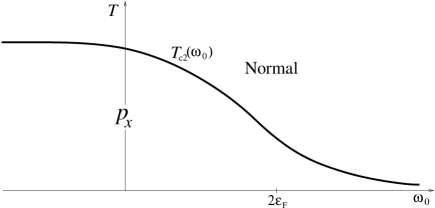
Figure 11: Temperature vs detuning phase diagram of the $p$-wave resonant Fermi gas for the case of a high resonance splitting, $\delta>\delta_{c}^{BCS}$. This phase diagram is also expected to describe a resonance with a splitting much larger than the Fermi energy for $\omega_{0}$ tuned to the $m=0$ resonance.

Consistent with above result of vanishing splitting, for weak dipolar splitting, $0<\delta<\delta_{c}^{BEC}$ we find that the $p$-wave $m=1$ superfluid ground state is stable, but slightly deformed to $p_{x}+i\alpha p_{y}$, with function $\alpha(\delta,\omega_{0})$ that we compute. For an intermediate dipolar splitting, $\delta_{c}^{BEC}<\delta<\delta_{c}^{BCS}$ the ground is a $p_{x}+ip_{y}$-superfluid ($m=1$) in the BCS regime and is a $p_{x}$-superfluid ($m=0$) in the BEC regime. We therefore predict a quantum phase transition at $\omega_{0c}$ between these two $p$-wave superfluids for intermediate range of dipolar splitting Gurarie et al. (2005); com (e). For a large Feshbach-resonance splitting, $\delta>\delta_{c}^{BSC}$ the ground state is a stable $p_{x}$-superfluid for all detuning. We show that in all these anisotropic cases the $p_{x}$-axis of the $p$-wave condensate order parameter is aligned along the external magnetic field. Finally, we expect that for an extremely large dipolar splitting, much bigger than $\epsilon_{F}\gamma_{p}$ (which could quite well be the current experimental situation), the system can be independently tuned into $m=0$ and $m=\pm 1$ resonances, and may therefore display the $p_{x}+ip_{y}$ and $p_{x}$ states separately, depending on to which of the $m=0$ or $m=\pm 1$ resonances the system is tuned. Thus even in the case of an extremely large dipolar splitting, phase diagrams in Fig. 8 and in Fig. 11 will be separately observed for tuning near the $m=1$ and $m=0$ resonances, respectively.

As illustrated in the phase diagrams above, we have also extended these results to a finite temperature, using a combination of detailed microscopic calculation of the free energy with more general Landau-like symmetry arguments. We show quite generally that for a dipolar-split (anisotropic) resonant gas, the normal to a $p$-wave superfluid transition at $T_{c2}(\omega_{0},\delta)$ is always into a $p_{x}$-superfluid, that, for an intermediate dipolar splitting is followed by a $p_{x}$-superfluid to $p_{x}+ip_{y}$ superfluid transition at $T_{c1}(\omega_{0},\delta)$. The ratio of these critical temperatures is set by

$${T_{c2}\over T_{c1}}\sim e^{\delta/a_{1}},$$ (19)

where $a_{1}$, given in Eq. (303), is an energy scale that we derive. As seen from the corresponding phase diagram, Fig. 10, we predict that $T_{c1}(\omega_{0})$ vanishes in a universal way according to

$$T_{c1}(\omega_{0})\sim|\omega_{0}-\omega_{0c}|^{1/2},$$ (20)

at a quantum critical point $\omega_{0c}$, that denotes a $T=0$ quantum phase transition between $p_{x}$ and $p_{x}+ip_{y}$ superfluids.

In addition to these conventional quantum and classical phase transitions, we predict that a $p$-wave resonant superfluid can exhibit as a function of detuning, $\omega_{0}$ quite unconventional (non-Landau type) phase transitions between a weakly-paired (BCS regime of $\mu>0$) and a strongly-paired (BEC regime of $\mu<0$) versions of the $p_{x}$ and $p_{x}+ip_{y}$ superfluids Volovik (1992, 2003); Klinkhamer and Volovik (2004); Volovik (2006). In three dimensions these are clearly distinguished by a gapless (for $\mu>0$) and a gapped (for $\mu<0$) quasiparticle spectra, and also, in the case of a $p_{x}+ip_{y}$ superfluid via a topological invariant that we explicitly calculate.

While the existence of such transitions at $\mu=0$ have been previously noted in the literature  Volovik (1992, 2003); Klinkhamer and Volovik (2004); Volovik (2006) our analysis demonstrates that these (previously purely theoretical models) can be straightforwardly realized by a $p$-wave resonant Fermi gas by varying the Feshbach resonance detuning, $\omega_{0}$.

Moreover, if the condensate is confined to two dimensions, at a positive chemical potential this state is a Pfaffian, isomorphic to the Moore-Read ground state of a fraction quantum Hall ground state believed to describe the ground state of the plateau at the filling fraction $\nu=5/2$. This state has been shown to exhibit topological orderRead and Green (2000); Volovik (2003), guaranteeing a $4$-fold ground state degeneracy on the torus and vortex excitations that exhibit non-Abelian statistics.

As was shown by Read and Green  Read and Green (2000), despite the fact that both weakly- and strongly-paired $p$-wave superfluid states are gapped in the case of a $p_{x}+ip_{y}$- (but not $p_{x}$-) superfluid the topological order classification and the associated phase transition at $\mu=0$ remains. Consistent with the existence of such order, we also show Gurarie and Radzihovsky (via an explicit construction) that for $\mu>0$, an odd vorticity vortex in a $p_{x}+ip_{y}$-superfluid will generically exhibit a single zero mode localized on it. In an even vorticity vortex such zero-energy solutions are absent.

In the presence of far separated vortices, these zero-modes will persist (up to exponential accuracy), leading to a degenerate many-particle ground state, and are responsible for the non-Abelian statistics of associated vortices Read and Green (2000); Volovik (2003, 2006); Gurarie and Radzihovsky . This new concrete realization of a topological ground state with non-Abelian excitations, may be important (beyond the basic physics interest) in light of a recent observation that non-Abelian excitations can form the building blocks of a “topological quantum computer”, free of decoherence Kitaev (2003). We thus propose a Feshbach resonant Fermi gas, tuned to a $p_{x}+ip_{y}$-superfluid ground state as a potential system to realize a topological quantum computer Gurarie et al. (2005); Tewari et al. (2006a).

II Resonant Scattering Theory: Phenomenology

A discussion of a two-body scattering physics, that defines our system in a dilute limit, is a prerequisite to a formulation of a proper model and a study of its many-body phenomenology. We therefore first focus on a two-particle quantum mechanics, that, for short-range interaction is fully characterized by a scattering amplitude $f({\bf k},{\bf k}^{\prime})$, where $\pm{\bf k}$ and $\pm{\bf k}^{\prime}$ are scattering momenta before and after the collision, respectively, measured in the center of mass frame. In the case of a centrally symmetric interaction potential $U(r)$, the scattering amplitude $f(k,\theta)$ only depends on the magnitude of the relative momentum, namely energy

$$E=\frac{k^{2}}{2m_{r}}$$

(with $m_{r}=m_{1}m_{2}/(m_{1}+m_{2})$ the reduced mass) and the scattering angle $\theta$ (through ${\bf k}\cdot{\bf k}^{\prime}=k^{2}\cos\theta$), and therefore can be expanded in Legendre polynomials, $P_{\ell}(\cos\theta)$

$$f(k,\theta)=\sum_{\ell=0}^{\infty}(2\ell+1)f_{\ell}(k)P_{\ell}(\cos\theta).$$ (21)

The scattering amplitude is related to the differential scattering cross section, the probability density of scattering into a solid angle $\Omega$, by a standard relation $d\sigma/d\Omega=|f|^{2}$. The $\ell$-th partial-wave scattering amplitude $f_{\ell}(k)$ measures the scattering in the angular momentum channel $\ell$, conserved by the spherically symmetric potential $U(r)$. For later convenience, when we focus on $s$- and $p$-wave channels, we denote $\ell=0$ and $\ell=1$ quantities with subscripts $s$ and $p$, respectively, as in

$$f_{s} \equiv f_{\ell=0}$$ (22)

$$f_{p} \equiv f_{\ell=1}.$$ (23)

In terms of the scattering matrix $S_{\ell}=e^{i2\delta_{\ell}}$ in channel $\ell$, defined by a phase shift $\delta_{\ell}$, the scattering amplitude is given by $f_{\ell}=(e^{i2\delta_{\ell}}-1)/(2ik)$.

Analyticity and unitarity of the scattering matrix, $|S_{\ell}|=1$, then restrict the scattering amplitude to a generic form

$$f_{\ell}(k)={1\over k^{-2\ell}F_{\ell}(k^{2})-ik},$$ (24)

where $F_{\ell}(k^{2})$ is a real function Taylor expandable in powers of its argument Landau and Lifshitz (1981). It is directly related to the scattering phase shifts $\delta_{\ell}(k)$ through the scattering matrix $S_{\ell}=e^{i2\delta_{\ell}}$ via $k^{2\ell+1}\cot\delta_{\ell}(k)=F_{\ell}(k^{2})$. Notice that at small $k$,

$$f_{\ell}(k)\sim k^{2\ell}.$$ (25)

Important information is contained in the poles $E_{\rm pole}$ of scattering amplitude (defined by $f_{\ell}^{-1}(E_{\rm pole})=0$), when it is studied as a function of complex energy $E$. Poles in $f_{\ell}(E)$ correspond to discrete eigenstates with different boundary conditions that can be obtained without explicitly solving the corresponding Schrodinger equation. However, because $k=\sqrt{2m_{r}E}$, the scattering amplitude, while a single-valued function of the momentum is a multi-valued function of the energy, and one must be careful to specify the branch on which a pole is located in identifying it with a particular eigenstate of a Schrodinger equation. Starting with a branch where $E>0$ and $k>0$, negative energy $E<0$ can be approached from the positive real axis either via the upper or lower half complex plane. A pole which lies on the negative real axis, approached via the upper half plane is equivalent to $k=+i\sqrt{2m_{r}|E|}$, i.e., ${\rm Im}(k)>0$, and therefore corresponds to a true bound state of the potential $U(r)$, with a wavefunction $\psi(r)\sim e^{-|k|r}$ that properly decays at long distances. On the other hand, a pole on the negative real axis, approached via the lower half plane is not associated with a bound state, since it corresponds to $k=-i\sqrt{2m_{r}|E|}$, i.e., ${\rm Im}(k)<0$ and therefore to an unphysical wavefunction that grows at large distances as $\psi(r)\sim e^{|k|r}$. Although it reflects a real low-energy feature of a scattering amplitude $f_{\ell}(E)$, the so-called virtual bound state Landau and Lifshitz (1981) does not correspond to any physical bound state solution of a Schrodinger equation as it does not satisfy decaying boundary conditions demanded of a physical bound state.

On the other hand a pole

$$E_{\rm pole}=E_{r}-i\Gamma/2,$$ (26)

of $f_{\ell}(E)$, with ${\rm Re}~{}E_{\rm pole}\equiv E_{r}>0$, ${\rm Im}~{}E_{\rm pole}\equiv-\Gamma/2<0$ is a resonance, that corresponds to a long-lived state with a positive energy $E_{r}={\rm Re}~{}E_{\rm pole}$ and width $\Gamma=-2~{}{\rm Im}~{}E_{\rm pole}$, latter characterizing the lifetime $\tau=1/\Gamma$ for this state to decay into a continuum. A complex conjugate pole that always appears along with this resonance pole, corresponds to an eigenstate that is time reversal of the resonance solution Landau and Lifshitz (1981); Res .

Coming back to the scattering amplitude Eq. (24), a low-energy scattering (small $k$) is characterized by a first few low-order Taylor expansion coefficients of $F_{\ell}(k^{2})$, and therefore only weakly depends on details of the interaction potential $U(r)$. This observation is at the heart of our ability to capture with a simple model Hamiltonian (see Sec V, below) the experimentally determined two-body phenomenology, governed by a complicated atomic interaction potential $U(r)$ or even multi-channel model as in the case of a Feshbach resonant systems. To do this we next specialize our discussion to a particular angular momentum channel.

II.1 Low energy $s$-wave scattering

We first concentrate on $s$-wave ($\ell=0$) scattering that, by virtue of Eq. (25), is the channel, that, for two fermion species dominates at low energies.

II.1.1 Scattering in the asymptotically low energy limit

Scattering at low energies can be analyzed by expanding the amplitude $F_{s}(k^{2})$ in powers of its argument, that to lowest order leads to a simple form

$$f_{s}(k)=-{1\over a^{-1}+ik},$$ (27)

with $a=-1/F_{s}(0)$, where $a$ is called the $s$-wave scattering length. The latter can be identified with particle effective interaction (in Born approximation proportional to a Fourier transform of the potential), with $a>0$ ($a<0$) generally (but not always) corresponding to a repulsive (attractive) potential. We observe that at zero momentum the scattering amplitude is simply equal to the scattering length, $f(0)=-a$, leading to $\sigma=4\pi a^{2}$ scattering cross section.

We can now give a physical interpretation to the only pole of Eq. (27) located at

$$k_{\rm pole} = ia^{-1},$$ (28)

$$E_{\rm pole} = -{1\over 2m_{r}a^{2}}.$$ (29)

The key observation at this stage is that by virtue of Eq. (28) and the fact that to be a physical bound state $\psi\sim e^{ik_{\rm pole}r}$ must decay at large $r$, the pole Eq. (28) corresponds to the true bound state with energy, $E_{\rm pole}$ only if $a>0$. In contrast, for $a<0$ the scattering amplitude pole corresponds to a wavefunction that grows exponential with $r$ and therefore, despite having a negative $E_{\rm pole}$, is not a physical bound state or a resonance solution of a Schrodinger equation, but is what is called a virtual bound state.Landau and Lifshitz (1981) Hence, a physical bound state characterized by a binding energy $1/(2m_{r}a^{2})$, that vanishes with $a^{-1}\rightarrow 0$, only exists for a positive scattering length $a$ and disappears for a negative $a$.

Thus, lacking any other poles at this lowest order of approximation, the scattering amplitude (27), while capturing the asymptotic low-energy bound states of the potential $U(r)$, does not exhibit any resonances Res , i.e., states with a positive energy and a finite lifetime. $f_{s}(k)$ in Eq. (27) corresponds to a scattering from a relatively featureless potential of the form illustrated in Fig. 12, where for a sufficiently deep well, there is a bound state and $a>0$, but only a continuum of states with $a<0$ and no resonance for well more shallow than a critical depth. This is despite the existence of an (unphysical) virtual bound state for $a<0$, with a negative energy $E=-1/(2m_{r}a^{2})$ identical to that of a true bound state (only present for $a>0$). This point is, unfortunately often missed in the discussions of Eq. (27) that have appeared in the literature. As we discuss in detail below, this scattering phenomenology is captured by a featureless short-ranged attractive $2$-body interaction (pseudo-potential) such as the commonly used delta-function four-Fermi many-body interaction.

Figure 12: A weakly attractive potential is progressively made more and more attractive, until a bound state appears, indicated in the figure by a dashed line. Although such potential leads to strong resonant scattering, when a bound state is close to or has just appeared, in contrast to a potential in Fig.5 it does not exhibit a resonance in a sense of a long-lived state with a positive energy and finite width Res .

We notice that in order to be able to trust Eqs. (28) and (29), all higher order terms in the expansion of $F_{s}(k^{2})$ calculated at this value of energy have to be negligible when compared with $|k|_{\rm pole}=a^{-1}$. In other words, $a$ has to be sufficiently large, and $|E|_{\rm pole}$ sufficiently small, with precise criteria determined by the details of the scattering potential and the corresponding coefficients of higher order terms in the Taylor expansion of $F_{s}(k^{2})$.

II.1.2 Intermediate energy resonant scattering

In order to capture the resonant states (absent in the approximation Eq. (27)), which could be present in the potential $U(r)$, $F_{s}(k^{2})$ in $f_{s}(k)$ must be expanded to the next order in $k^{2}$,

$$F_{s}(k^{2})=-a^{-1}+\frac{1}{2}r_{0}k^{2},$$ (30)

with parameter $r_{0}$ usually called the effective range of the interaction potential. For a generic, everywhere attractive potential, $U(r)<0$, $r_{0}$ can be shown to be positive Landau and Lifshitz (1981), and moreover, to roughly coincide with the spatial extent of $U(r)$, hence the name “effective range”. However, as is clear from physical considerations and an analysis of pole structure of $f_{s}(k^{2})$, a potential which is attractive everywhere cannot support a resonance. In order to be able to capture a positive energy quantum particle for a significant amount of time, the potential must be attractive at short scales and exhibit a positive energy barrier at intermediate scales, of a generic form illustrated in Fig. 5. It can be shown that for such a potential, $r_{0}$ is in fact negative, with its magnitude having nothing to do with the range of $U(r)$. Instead for such resonant $U(r)$ as shown on Fig. 5, $|r_{0}|^{-1}$ reflects the barrier transmission coefficient, with the higher barrier corresponding to a longer resonance lifetime and larger $|r_{0}|$. Therefore, focusing on resonant potentials, we will take $r_{0}<0$, keeping in mind that $|r_{0}|$ can be much longer than the actual microscopic range of the scattering potential, $d\equiv 2\pi/\Lambda$. In short, to leave open the possibility for the scattering to go in the presence of low-energy resonances, in addition to bound states and virtual bound states, $r_{0}$ must be negative and “anomalously” large, a condition that will be assumed throughout the rest of this paper.

At this higher level of approximation, the scattering amplitude is given by

$$f_{s}(k)=-{1\over-\frac{1}{2}r_{0}k^{2}+a^{-1}+ik},$$ (31)

Equivalently, in terms of energy $E=k^{2}/2m_{r}$ (in a slight abuse of notation) $f_{s}$ takes the form

$$f_{s}(E)=-{1\over\sqrt{2m_{r}}}{\Gamma_{0}^{1/2}\over E-\omega_{0}+i\Gamma_{0}^{1/2}E^{1/2}},$$ (32)

in which

$$\omega_{0}\equiv{1\over m_{r}r_{0}a}=\frac{1}{2}\Gamma_{0}\frac{r_{0}}{a},$$ (33)

and, as discussed in the Introduction, Sec. I.2, a characteristic energy scale

$$\Gamma_{0}\equiv{2\over m_{r}r_{0}^{2}}$$ (34)

is made explicit, with $r_{0}=-\sqrt{2/m_{r}\Gamma_{0}}$. It marks a crossover energy scale between a low- and intermediate-energy behaviors of $f_{s}(E)$. Also, as we will see below, $\Gamma_{0}$ defines an energy scale for the low-energy pole above (below) which, $1/m_{r}a^{2}\gtrsim\Gamma_{0}$ ($1/m_{r}a^{2}\lesssim\Gamma_{0}$) a resonant state appears (disappears).

The poles of the scattering amplitude are given by

$$k_{\rm pole}^{\pm} = {i\over r_{0}}\pm{\sqrt{2ar_{0}-a^{2}}\over ar_{0}},$$ (35)

$$E_{\rm pole} = {1\over m_{r}r_{0}^{2}}\left({r_{0}\over a}-1+\sqrt{1-2{r_{0}\over a}}\right),$$ (36)

$$= \omega_{0}-\frac{1}{2}\Gamma_{0}\left(1-\sqrt{1-4\omega_{0}/\Gamma_{0}}\right),$$

where in $E_{\rm pole}$, Eq.(36) we only kept the “minus” pole (with the minus sign in front of the square-root of) $k_{\rm pole}^{-}$, as the other pole $k_{\rm pole}^{+}$ (with a plus sign) corresponds to an unphysical virtual bound state (regardless of the sign of the scattering length $a$), and therefore will be ignored in all further discussions.

The real part of the energy $E_{\rm pole}$, Eq. (36), as a function of $-a^{-1}$ (with $r_{0}<0$) is illustrated in Fig. 13. As $-a^{-1}$ is changed from $-\infty$ to $+\infty$, the pole first represents a bound state, then a virtual bound state (plotted as dotted curve), and finally a resonance. This is further illustrated in Fig. 14, where the position of the pole $E_{\rm pole}$ is shown in a complex plane of energy $E$, with arrows on the figure indicating its motion with increasing $-a^{-1}$. The bound state and virtual bound state correspond to Im $E_{\rm pole}=0^{\pm}$, respectively, with the former (latter) approaching negative real axis from above (below) the branch cut. The resonance, on the other hand, corresponds to Im $E_{\rm pole}<0$ and a positive real part of the energy, Re $E_{\rm pole}>0$.

Figure 13: The pole of the scattering amplitude $f_{s}(E)$, Eq. (36) as a function of $-1/a$ for $r_{0}<0$. As discussed in the text, only a bound state and a resonance correspond to physical solutions of the Schrodinger’s equation with proper boundary conditions. The thin dotted line indicates asymptotic linear behavior of the bound state for small positive $a$.

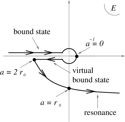
Figure 14: The pole of the scattering amplitude $f_{s}(k)$, Eq. (36), shown in a complex plane of $E$. The arrows indicate pole’s motion as $-1/a$ is increased.

We note that for $1/|a|\ll 1/|r_{0}|$, the Eq. (36), lying close to zero, approximately coincides with Eq. (29), as expected, since the higher order term $\frac{1}{2}r_{0}k_{\rm pole}^{2}$ in $f_{s}(k)$ is subdominant to $ik_{\rm pole}$. In other words, at a sufficiently large scattering length, the scattering is well-approximated by the asymptotic low-energy (scattering-length) approximation of the previous section. For such large positive $a\gg|r_{0}|$ it gives bound state energy, Eq. (29), that grows quadratically with $1/a$. Further away from the resonance, on the positive $a$ side, where the scattering length drops significantly below the effective range, $a\ll|r_{0}|$, the bound state energy crosses over to a linear dependence on $1/a$, as illustrated in Fig.13 and summarized by

$$E_{\rm bound}(a) = \cases{-\frac{1}{2m_{r}a^{2}},&\text{for $|r_{0}|\ll a>0$}\cr-\frac{1}{m_{r}|r_{0}|a},&\text{for $|r_{0}|\gg a>0$}.\cr}$$ (37)

More importantly, however, on the other side of the resonance, where the scattering length is negative, unlike Eq. (29), Eq. (36) also describes a resonant state, that appears for $a<0$ and shorter than the effective range $r_{0}$, i.e., for $-\frac{1}{a}>-\frac{1}{r_{0}}$, when the real part of the energy $E_{\rm pole}$ becomes positive. The resonant state is characterized by a peak at energy $E_{r}=E_{\rm resonance}$ and a width $\Gamma_{s}$ given by

$$E_{\rm resonance} = {1\over m_{r}r_{0}^{2}}\left({{r_{0}\over a}-1}\right),$$

$$= \omega_{0}-\frac{1}{2}\Gamma_{0},$$

$$\Gamma_{s} = {2\over m_{r}r_{0}^{2}}\sqrt{{2r_{0}\over a}-1}$$

$$= \Gamma_{0}\sqrt{{4\omega_{0}\over\Gamma_{0}}-1}.$$

Hence, we find that in the $s$-wave resonant case, generically, even potentials that exhibit a resonance for small $|a|$ (high energy), lose that resonance and therefore reduce to a nonresonant case for sufficiently large and negative $a$ (low energy).

The transition from a bound state to a resonance as a function of $a$ is exhibited by scattering via a generic resonant potential illustrated in Fig.5. A sufficiently deep well will exhibit a true bound state, whose energy will vanish with decreasing depth and correspondingly increasing $a$, according to $E_{\rm bound}=-1/(2m_{r}a^{2})$, Eq.(29). We note, however, that as the potential is made even more shallow, $1/a$ crosses $0$ and the true bound state disappears (turning into an unphysical virtual bound state), the resonant state (positive energy and finite lifetime) does not appear until a later point at which scattering length becomes shorter than the effective range, i.e., until $|a|<|r_{0}|$.

This somewhat counterintuitive observation can be understood by noting that the lifetime of an $s$-wave resonant state is finite, given by the inverse probability of tunneling through a finite barrier, which only weakly depends on the energy of the state as long as the potential in Fig. 5 is not too long-ranged. Thus, even when the energy of the resonance goes to zero, its width remains finite. Hence, since the bound state’s width is exactly zero, small deepening of the potential cannot immediately change a resonance into a bound state, simply by reasons of continuity. There has to be some further deepening of the potential $U(r)$ (range of $a$), over which the resonance has already disappeared, but the bound state has not yet appeared. During this intermediate range of potential depth corresponding to $0<1/|a|<1/|r_{0}|$, when the potential is not deep enough to support a true bound state but not yet shallow enough to exhibit a resonance, the scattering is dominated by a virtual bound state pole, as illustrated in Figs. 13, 14.

II.2 $P$-wave scattering

As remarked earlier, in a low-energy scattering of a particle off a potential $U(r)$, the $s$-wave ($\ell=0$) channel dominates over higher angular momentum $\ell\neq 0$ contributions, that by virtue of the generic form of the scattering amplitude, Eq. (24) vanish as $k^{2\ell}$, Eq. (25). This suppression for $\ell\neq 0$ arises due to a long-ranged centrifugal barrier, that at low energies prevents a particle from approaching the origin where the short range scattering potential $U(r)$ resides.

Hence, in the case of a Feshbach resonance of two hyperfine species Fermi gas, where the scattered particles are distinguishable (by their hyperfine state), at low energies, indeed, the interaction is dominated by the $s$-wave resonance, with higher angular momentum channels safely ignored. However, an exception to this is the scattering of identical fermions, corresponding to atoms in the same hyperfine state in the present context. Because Pauli exclusion principle forbids fermion scattering in the $s$-wave channel, the next higher angular momentum channel, namely $p$-wave ($\ell=1$) scattering dominates, with $s$-wave and $\ell>1$ channels vanishing at low energies com (d). Thus we see that $p$-wave Feshbach resonance is quite special, being the dominant interaction channel for a single species Fermi gas. With this motivation for our focus on a $p$-wave Feshbach resonant superfluidity and in preparation for its study, we next analyze a $p$-wave scattering amplitude.

Starting with Eq. (24) and expanding $F_{p}(k^{2})$ similarly to Eq. (30) we find

$$F_{p}(k^{2})=-v^{-1}+\frac{1}{2}k_{0}k^{2}.$$ (40)

Here $v$ is the so-called scattering volume analogous to the scattering length $a$ of the $s$-wave case, diverging and changing sign when the system is taken through a $p$-wave Feshbach resonance. A characteristic wavevector $k_{0}$ is everywhere negative and plays a role similar to that of the effective range $r_{0}$ in the $s$-wave channel, but has dimensions of an inverse length.

Hence at low energies the $p$-wave scattering amplitude takes the form

$$f_{p}(k)={k^{2}\over-v^{-1}+\frac{1}{2}k_{0}k^{2}-ik^{3}}.$$ (41)

Although the poles of the scattering amplitude Eq. (41) can be found by solving a qubic equation, their exact positions are not very illuminating and will not be pursued here. Instead, it will be sufficient for our purpose to only consider an important low-energy limit $|v^{-1}|\ll|k_{0}|^{3}$, in which the relevant pole of Eq. (41) is close to zero and its position can be found by neglecting (actually treating perturbatively in powers of $|vk_{0}^{3}|$) $ik^{3}$ term in the scattering amplitude. To lowest order the pole is then simply given by

$$E_{\rm pole}\approx{1\over m_{r}vk_{0}}.$$ (42)

This corresponds to a real bound state for $E_{\rm pole}<0$ (when $v>0$) and a resonance for $E_{\rm pole}>0$ (when $v<0$), with a width easily estimated to be

$$\Gamma_{p} \approx {2k_{\rm pole}^{3}\over m_{r}k_{0}}=E_{\rm pole}\sqrt{32/|vk_{0}^{3}|},$$ (43)

$$\ll E_{\rm pole},$$ (44)

near a resonance, where $|vk_{0}^{3}|\rightarrow\infty$. Thus, in contrast to the $s$-wave case, where at sufficiently low energies ($E<\Gamma_{0}=2/m_{r}r_{0}^{2}$) the width $\Gamma_{s}\approx\sqrt{\Gamma_{0}E}\gg E$, here, because $\Gamma_{p}\sim E^{3/2}$, a $p$-wave resonance becomes arbitrarily narrow at low energies. Consequently, as the inverse scattering volume $v^{-1}$ is tuned through zero and the relevant two-body energy $E_{\rm pole}=1/(2\ m_{r}vk_{0})$ vanishes, the real bound state immediately turns into a resonance without going through an intermediate virtual bound state (as it did in the $s$-wave case). This is illustrated on Fig. 15. This resonant pole behavior extends to all finite angular momentum ($\ell>0$) channels.

Figure 15: The pole of a $p$-wave scattering amplitude Eq. (41) as a function of $-1/v$ for $k_{0}<0$.

The physical reason behind such a drastic difference between $s$-wave and $p$-wave (and higher $\ell>0$ channels) resonances stems from the centrifugal barrier that adds a long-ranged $1/r^{2}$ tail to the effective scattering potential $U_{\rm eff}(r)=U(r)+{\hbar^{2}\ell(\ell+1)\over 2m_{r}r^{2}}$. The width of a low lying resonant state in such potential can be estimated by computing the decay rate through $U_{\rm eff}(r)$, dominated by the long-ranged centrifugal barrier $\sim 1/r^{2}$. Employing the WKB approximation, at low energy $E$ the decay rate is well approximated by

$$\Gamma \sim e^{-{2\over\hbar}\int_{d}^{r_{E}}dr\sqrt{2m_{r}U_{\rm eff}}},$$ (45)

$$\approx e^{-2{\sqrt{\ell(\ell+1)}\int_{d}^{r_{E}}dr/r}},$$ (46)

$$\approx \left({r_{E}\over d}\right)^{-2\sqrt{\ell(\ell+1)}},$$ (47)

In above $d$ and $r_{E}$ are the classical turning points of the $-U_{\rm eff}(r)$, where $d$ can be taken as the microscopic range of the potential (closed-channel molecular size), and more importantly $r_{E}$ is determined by

$$E={\hbar^{2}\ell(\ell+1)\over 2m_{r}r_{E}^{2}}.$$ (48)

Combining this with Eq. (47) gives

$$\Gamma_{\ell}\sim E^{\sqrt{\ell(\ell+1)}}.$$ (49)

Although WKB approximation does not recover the correct exponent of $\ell+1/2$, Eq. (24) (required by unitarity and analyticity) except for the expected large $\ell$ limit (consistent with the fact that for small $\ell$ the semiclassical criterion on which it is based fails), it does correctly predict a narrowing of the resonance at low energies and with increasing angular momentum $\ell$.

Of course, the expansion Eq. (40) is only a good approximation for small $k$. But in this regime it captures both low energy real bound state (for $1/v>0$) and narrow resonant state (for $1/v<0$). Experimentally this regime is guaranteed to be accessible by tuning the bound state and resonance energy $E_{\rm pole}=1/(m_{r}vk_{0})$ sufficiently close to zero so that $|vk_{0}^{3}|\ll 1$. In this range the scattering amplitude Eq. (41) correctly captures the physics of a resonant scattering potential and the related Feshbach resonance without the need for higher order terms in the expansion of $F_{p}(k^{2})$.

III Resonant Scattering Theory: Microscopics

III.1 Potential scattering

The next step in our program is to develop a model of a gas of fermions interacting via a resonant pairwise potential $U(r)$ of the type illustrated in Fig. 5, that exhibits a real bound state or a resonance, controlled by tuning its shape (e.g., well depth). It is of course possible to simply use a many-body theory with a pairwise interactions literally taken to be $U(r)$ of Fig. 5, with a (normal-ordered) Hamiltonian given by

$$\hat{H} = \int d^{3}r~{}\sum_{\sigma}\hat{\psi}^{\dagger}_{\sigma}\left(-{\nabla^{2}\over 2m}\right)\hat{\psi}_{\sigma}$$

$$+ \frac{1}{2}\sum_{\sigma,\sigma^{\prime}}\int d^{3}rd^{3}r^{\prime}U(|{\bf r}-{\bf r}^{\prime}|)~{}\hat{\psi}^{\dagger}_{\sigma}({\bf r})\hat{\psi}^{\dagger}_{\sigma^{\prime}}({\bf r}^{\prime})\hat{\psi}_{\sigma^{\prime}}({\bf r}^{\prime})\hat{\psi}_{\sigma}({\bf r}).$$

where $\hat{\psi}_{\sigma}({\bf r})$ ($\hat{\psi}^{\dagger}_{\sigma}({\bf r})$) is an annihilation (creation) field operator of a fermion of flavor $\sigma$ at a point ${\bf r}$. We would like first to discuss how a problem defined by the Hamiltonian, (III.1) leads directly to scattering amplitudes Eq. (24).

Motivated by experiments where studies are confined to gases of no more than two fermion flavors (corresponding to a mixture of two distinct hyperfine states) we will refer to $\sigma$ as simply spin, designating a projection ($\sigma$) of the corresponding two-flavor pseudo-spin along a quantization axis as a spin up, $\uparrow$, and down, $\downarrow$. In an equivalently and sometimes more convenient momentum basis above Hamiltonian becomes

$$\hat{H}=\sum_{\sigma}\sum_{\bf k}\frac{k^{2}}{2m}\hat{a}^{\dagger}_{{\bf k},\sigma}\hat{a}_{{\bf k},\sigma}+\frac{1}{2V}\sum_{\sigma,\sigma^{\prime}}\sum_{{\bf k},{\bf k}^{\prime},{\bf p}}\tilde{U}(|{\bf k}-{\bf k}^{\prime}|)\hat{a}^{\dagger}_{{\bf k}^{\prime}+\frac{{\bf p}}{2},\sigma}\hat{a}^{\dagger}_{-{\bf k}^{\prime}+\frac{{\bf p}}{2},\sigma^{\prime}}\hat{a}_{-{\bf k}+\frac{{\bf p}}{2},\sigma^{\prime}}\hat{a}_{{\bf k}+\frac{{\bf p}}{2},\sigma},$$ (51)

where $\hat{a}_{{\bf k},\sigma}$ ($\hat{a}^{\dagger}_{{\bf k},\sigma}$) is an annihilation (creation) operator of a fermionic atom of flavor $\sigma$ with momentum ${\bf k}$, satisfying canonical anticommutation relations and related to the field operator by $\hat{\psi}_{\sigma}({\bf r})=V^{-1/2}\sum_{\bf k}\hat{a}_{{\bf k},\sigma}e^{i{\bf k}\cdot{\bf r}}$. With our choice of momentum variables above the relative center of mass momenta before (after) the collision are $\pm{\bf k}$ ($\pm{\bf k}^{\prime}$) and ${\bf p}$ is the conserved momentum of the center of mass of the pair of scattering particles.

In the rest of this section, we would like to calculate the scattering amplitudes $f_{\ell}$ given in Eq. (21) in terms of the interaction potential $\tilde{U}(|{\bf k}-{\bf k}^{\prime}|)$. With this goal in mind, it is convenient to make the symmetry properties of the fermion interaction $\hat{H}_{int}$ explicit, by taking advantage of the rotational invariance of the two-body potential $U(|{\bf r}-{\bf r}^{\prime}|)$ and the anticommutation of the fermion operators. To this end we decompose the angular dependence (arising through $\hat{\bf k}\cdot\hat{\bf k}^{\prime}$, where $\hat{\bf k}$ is a unit vector parallel to ${\bf k}$) of the Fourier transform of the two-body potential, $\tilde{U}(|{\bf k}-{\bf k}^{\prime}|)$ into spherical harmonics via

$$\tilde{U}(|{\bf k}-{\bf k}^{\prime}|)\equiv U_{{\bf k},{\bf k}^{\prime}}=\sum_{\ell=0}^{\infty}(2\ell+1)u^{(\ell)}_{k,k^{\prime}}P_{\ell}(\hat{\bf k}\cdot\hat{\bf k}^{\prime}).$$ (52)

The $\ell$-th orbital angular momentum channel interaction amplitude $u^{(\ell)}_{k,k^{\prime}}$ can be straightforwardly shown to be given by

$$u^{(\ell)}_{k,k^{\prime}}=4\pi\int_{0}^{\infty}dr~{}r^{2}U(r)j_{\ell}(kr)j_{\ell}(k^{\prime}r),$$ (53)

where $j_{\ell}(x)$ is the $\ell$-th spherical Bessel function.

Using anticommutativity of the fermion operators, it is possible to decompose the interaction term in Eq. (51) into the singlet and triplet channels by introducing the two-body interaction vertex $\tilde{U}_{\sigma_{1}\sigma_{2}}^{\sigma^{\prime}_{1}\sigma^{\prime}_{2}}({\bf k},{\bf k}^{\prime})$ defined by

$$\hat{H}_{int}=\frac{1}{2V}\sum_{\sigma_{1},\sigma_{2},\sigma^{\prime}_{1},\sigma^{\prime}_{2}}\sum_{{\bf k},{\bf k}^{\prime},{\bf p}}\tilde{U}_{\sigma_{1}\sigma_{2}}^{\sigma^{\prime}_{1}\sigma^{\prime}_{2}}({\bf k},{\bf k}^{\prime})\hat{a}^{\dagger}_{{\bf k}^{\prime}+\frac{{\bf p}}{2},\sigma^{\prime}_{1}}\hat{a}^{\dagger}_{-{\bf k}^{\prime}+\frac{{\bf p}}{2},\sigma^{\prime}_{2}}\hat{a}_{-{\bf k}+\frac{{\bf p}}{2},\sigma_{2}}\hat{a}_{{\bf k}+\frac{{\bf p}}{2}\sigma_{1}},$$ (54)

with

$$\tilde{U}_{\sigma_{1}\sigma_{2}}^{\sigma^{\prime}_{1}\sigma^{\prime}_{2}}({\bf k},{\bf k}^{\prime})=\frac{1}{2}\tilde{U}(|{\bf k}-{\bf k}^{\prime}|)\delta_{\sigma^{\prime}_{1}\sigma_{1}}\delta_{\sigma^{\prime}_{2}\sigma_{2}}-\frac{1}{2}\tilde{U}(|{\bf k}+{\bf k}^{\prime}|)\delta_{\sigma^{\prime}_{1}\sigma_{2}}\delta_{\sigma^{\prime}_{2}\sigma_{1}}),$$ (55)

that automatically reflects the antisymmetric (under exchange) property of fermions, namely

$$\tilde{U}_{\sigma_{1}\sigma_{2}}^{\sigma^{\prime}_{1}\sigma^{\prime}_{2}}({\bf k},{\bf k}^{\prime}) = -\tilde{U}_{\sigma_{2}\sigma_{1}}^{\sigma^{\prime}_{1}\sigma^{\prime}_{2}}(-{\bf k},{\bf k}^{\prime}),$$ (56)

$$= -\tilde{U}_{\sigma_{1}\sigma_{2}}^{\sigma^{\prime}_{2}\sigma^{\prime}_{1}}({\bf k},-{\bf k}^{\prime}).$$ (57)

The vertex can be furthermore decomposed into spin singlet (s) and triplet (t) channel eigenstates of the two-particle spin angular momentum,

$$\tilde{U}_{\sigma_{1}\sigma_{2}}^{\sigma^{\prime}_{1}\sigma^{\prime}_{2}}({\bf k},{\bf k}^{\prime})=\tilde{U}^{(s)}_{\sigma_{1}\sigma_{2},\sigma^{\prime}_{1}\sigma^{\prime}_{2}}({\bf k},{\bf k}^{\prime})+\tilde{U}^{(t)}_{\sigma_{1}\sigma_{2},\sigma^{\prime}_{1}\sigma^{\prime}_{2}}({\bf k},{\bf k}^{\prime}).$$ (58)

The singlet and triplet vertices

$$\tilde{U}^{(s)}_{\sigma_{1}\sigma_{2},\sigma^{\prime}_{1}\sigma^{\prime}_{2}}({\bf k},{\bf k}^{\prime}) = U^{(e)}({\bf k},{\bf k}^{\prime})\chi^{(s)}_{\sigma_{1}\sigma_{2},\sigma^{\prime}_{1}\sigma^{\prime}_{2}}$$ (59)

$$\tilde{U}^{(t)}_{\sigma_{1}\sigma_{2},\sigma^{\prime}_{1}\sigma^{\prime}_{2}}({\bf k},{\bf k}^{\prime}) = U^{(o)}({\bf k},{\bf k}^{\prime})\chi^{(t)}_{\sigma_{1}\sigma_{2},\sigma^{\prime}_{1}\sigma^{\prime}_{2}},$$

are expressed in terms of an orthonormal set of singlet and triplet projection operators

$$\chi^{(s)}_{\sigma_{1}\sigma_{2},\sigma^{\prime}_{1}\sigma^{\prime}_{2}} = \frac{1}{2}(\delta_{\sigma^{\prime}_{1}\sigma_{1}}\delta_{\sigma^{\prime}_{2}\sigma_{2}}-\delta_{\sigma^{\prime}_{1}\sigma_{2}}\delta_{\sigma^{\prime}_{2}\sigma_{1}}),$$ (60)

$$\chi^{(t)}_{\sigma_{1}\sigma_{2},\sigma^{\prime}_{1}\sigma^{\prime}_{2}} = \frac{1}{2}(\delta_{\sigma^{\prime}_{1}\sigma_{1}}\delta_{\sigma^{\prime}_{2}\sigma_{2}}+\delta_{\sigma^{\prime}_{1}\sigma_{2}}\delta_{\sigma^{\prime}_{2}\sigma_{1}}),$$

with coefficients

$$U^{(e)}({\bf k},{\bf k}^{\prime}) = \frac{1}{2}\left(\tilde{U}(|{\bf k}-{\bf k}^{\prime}|)+\tilde{U}(|{\bf k}+{\bf k}^{\prime}|)\right),\hskip 28.45274pt$$ (61)

$$U^{(o)}({\bf k},{\bf k}^{\prime}) = \frac{1}{2}\left(\tilde{U}(|{\bf k}-{\bf k}^{\prime}|)-\tilde{U}(|{\bf k}+{\bf k}^{\prime}|)\right),$$

that, by virtue of decomposition, Eq. (52) and symmetry of Legendre polynomials, $P_{\ell}(-\hat{\bf k}\cdot\hat{\bf k}^{\prime})=(-1)^{\ell}P_{\ell}(\hat{\bf k}\cdot\hat{\bf k}^{\prime})$ are vertices for even and odd orbital angular momentum $\ell$ channels, respectively, as required by the Pauli exclusion principle. Physically, these irreducible even and odd verticies make explicit the constructive and distructive interference between scattering by angle $\theta$ and $\pi-\theta$ of two fermions.

The two-body scattering amplitude $f({\bf k},{\bf k}^{\prime})$ is proportional to the $T$-matrix,

$$f({\bf k},{\bf k}^{\prime})=-{m\over 4\pi}T_{{\bf k},{\bf k}^{\prime}}=-\frac{m_{r}}{2\pi}T_{{\bf k},{\bf k}^{\prime}},$$ (62)

where $m_{r}=m/2$ is the reduced mass of two fermions. The $T$-matrix can be computed via standard methods. As illustrated on Fig. 16, it equals to a renormalized 4-point vertex (1PI) $\Gamma^{(4)}({\bf k}+{\bf p}/2,-{\bf k}+{\bf p}/2,{\bf k}^{\prime}+{\bf p}/2,-{\bf k}^{\prime}+{\bf p}/2;\varepsilon)$ for particles scattering with initial (final) momenta $\pm{\bf k}+{\bf p}/2$ ($\pm{\bf k}^{\prime}+{\bf p}/2$), and at a total energy in the center of mass frame given by

$$\varepsilon = \frac{({\bf k}+{\bf p}/2)^{2}}{2m}+\frac{(-{\bf k}+{\bf p}/2)^{2}}{2m}-\frac{p^{2}}{4m},$$

$$= \frac{k^{2}}{m}=\frac{k^{\prime 2}}{m}=\frac{k^{2}}{2m_{r}},$$

with the last relation valid due to energy conservation by a time independent interaction.

Figure 16: The renormalized 4-point vertex for potential scattering, determining the $T$-matrix $T_{{\bf k},{\bf k}^{\prime}}$.

Given the retarded Green’s functions of fermions,

$$G({\bf k},\omega)=\frac{1}{\omega-\frac{k^{2}}{2m}+i0},$$ (64)

the main ingredient of the sequence of diagrams from Fig. 16 is the polarization operator, denoted by a bubble in the figure, and physically corresponding the Green’s function of the reduced fermion with momentum ${\bf q}$ and mass $m_{r}$,

$$\Pi({\bf q},\varepsilon) = \int\frac{d\omega}{2\pi i}G\left(\frac{{\bf p}}{2}+{\bf q},\varepsilon+\frac{p^{2}}{4m}+\omega\right)G\left(\frac{{\bf p}}{2}-{\bf q},-\omega\right)$$ (65)

$$= \frac{1}{\varepsilon-\frac{q^{2}}{m}+i0}.$$

Although perhaps not immediately obvious, $\Pi({\bf q},\varepsilon)$ as defined above is independent of ${\bf p}$, the center of mass momentum of a pair of fermions.

The sequence of diagrams in Fig. 16 then generates a series for a $T$-matrix given by

$$T_{{\bf k},{\bf k}^{\prime}}=U_{{\bf k},{\bf k}^{\prime}}+\sum_{{\bf q}}U_{{\bf k},{\bf q}}\Pi({\bf q},\varepsilon)U_{{\bf q},{\bf k}^{\prime}}+\dots,$$ (66)

that can formally be resummed into an integral equation

$$T_{{\bf k},{\bf k}^{\prime}}=[(1-U\Pi)^{-1}U]_{{\bf k},{\bf k}^{\prime}},$$ (67)

where a martix product over wavevectors inside the square brackets is implied.

Utilizing the channel decomposition, Eq. (61) of the vertex $U_{{\bf k},{\bf k}^{\prime}}$ together with the closure-orthogonality relation

$$\int_{-1}^{1}P_{\ell}(\hat{{\bf k}}\cdot\hat{{\bf q}})P_{\ell^{\prime}}(\hat{{\bf q}}\cdot\hat{{\bf k}}^{\prime})d\Omega_{\bf q}=\frac{4\pi}{2\ell+1}\delta_{\ell\ell^{\prime}}P_{\ell}(\hat{{\bf k}}\cdot\hat{{\bf k}}^{\prime}),$$ (68)

the $T$-matrix series separates into a partial waves sum

$$T_{{\bf k},{\bf k}^{\prime}}=\sum_{\ell=0}^{\infty}(2\ell+1)T^{(\ell)}_{k,k^{\prime}}P_{\ell}(\hat{{\bf k}}\cdot\hat{{\bf k}}^{\prime}),$$ (69)

with

$$T^{(\ell)}_{k,k^{\prime}}=u^{(\ell)}_{k,k^{\prime}}+{1\over V}\sum_{{\bf q}}u^{(\ell)}_{k,q}\Pi(q,\varepsilon)u^{(\ell)}_{q,k^{\prime}}+\dots,$$ (70)

a $T$-matrix for scattering in an angular momentum channel $\ell$, conserved by the spherical symmetry of the two-body interaction potential. This demonstrates explicitly that the interaction vertices in different $\ell$ channels do not mix, each contributing only to the corresponding scattering amplitude channel $f_{\ell}(k)$ in Eq. (24).

Without specifying the interaction potential $U(r)$, a more explicit expression for the $T$-matrix can only be obtained for the so-called separable potential, discussed in detail in Ref. Nozières and Schmitt-Rink (1985). Such separable interaction is a model that captures well a low-energy behavior of a scattering amplitude of a more generic short-range potential. To see this, we observe that a generic short-range potential, with a range $d$, leads to a vertex in the $\ell$-th channel, which at long scales, $kd\ll 1$, separates into

$$u^{(\ell)}_{k,k^{\prime}}\approx\lambda k^{\ell}g^{(\ell)}_{k}k^{\prime\ell}g^{(\ell)}_{k^{\prime}}\approx\lambda k^{\ell}k^{\prime\ell},$$ (71)

with

$$\lambda = {4\pi U_{0}d^{2\ell+3}\over[(2\ell+1)!!]^{2}},$$ (72)

$$U_{0}d_{0}^{2\ell+3} \equiv \int_{0}^{\infty}dr~{}r^{2\ell+2}U(r).$$ (73)

Assuming that this separation holds at all $k$ (a definition of a separable potential), we use this asymptotics inside Eq. (70). This reduces the $T$-matrix to a geometric series that resums to

$$T^{(\ell)}_{k,k^{\prime}}={u^{(\ell)}_{k,k^{\prime}}\over 1-\lambda\Pi^{(\ell)}(\varepsilon)},$$ (74)

where $\Pi^{(\ell)}(\varepsilon)$ is the trace over momentum of the atom polarization “bubble” corresponding to the molecular self-energy at energy $\varepsilon$,

$$\Pi^{(\ell)}(\varepsilon) = \frac{1}{V}\sum_{\bf q}q^{\ell}g^{(\ell)}_{q}\Pi(q,\varepsilon)q^{\ell}g^{(\ell)}_{q},$$ (75)

$$= \int{d^{3}q\over(2\pi)^{3}}{q^{2\ell}g^{(\ell)}(q)^{2}\over\varepsilon-{q^{2}\over m}+i0},$$ (76)

$$= -m\Lambda^{2\ell+1}R\left(\frac{k^{2}}{\Lambda^{2}}\right)-{i\over 4\pi}m^{\ell+3/2}\ \varepsilon^{\ell+1/2}.$$ (77)

In above $R(x)$ is a Taylor-expandable function of its dimensionless argument, the momentum cutoff $\Lambda\approx 2\pi/d$ is set by the potential range $d$, and, as before, $k^{2}/m=\varepsilon$. Putting this together inside the $T$-matrix, we find the low-energy $\ell$-channel scattering amplitude

$$f^{(\ell)}(k)=-\frac{1}{\frac{4\pi}{mk^{2\ell}}\left(\frac{1}{\lambda}+m\Lambda^{2\ell+1}R\left(\frac{k^{2}}{\Lambda^{2}}\right)\right)+ik},\ k\ll\Lambda.$$ (78)

This coincides with the general form, Eq. (24) arising from the requirement of analyticity and unitarity of the scattering matrix. However, we observe that in the $s$-wave case, for the full range of accessible wavevectors up to ultraviolet cutoff, $k<\Lambda$ the scattering amplitude Eq. (78) is well approximated by the non-resonant, scattering-length dominated form (27), with the scattering length given by $a^{-1}=4\pi/(m\lambda)+4\pi\Lambda R(0)$. The “effective range” $r_{0}$ extracted from Eq. (78) is $r_{0}\sim 1/\Lambda$, namely microscopic, positive, and is of the order of the spatial range of the potential $d$. Yet, as we saw in Sec. II.1, in order to capture possible resonances, $r_{0}$ must be negative and much longer than the actual spatial range of the potential. The fact that our calculation does not capture possible resonances is an artifact of our choice of a separable potential.

Although a more physical (nonseparable) potential $U(r)$, of a resonant form depicted in Fig. 5, indeed exhibits scattering via a resonant state (not just a bound and virtual bound states), calculating the scattering amplitude $f_{\ell}(k)$ (beyond Eq. (71) approximation) is not really practical within the second-quantized many-body approach formulated in Eq. (III.1). In fact, the only way to derive the scattering amplitude in that case is to go back to the Schrödinger equation of a pair of fermions, reducing the problem to an effective single-particle quantum mechanics. However, because we are ultimately interested in condensed states of a finite density interacting atomic gas, this two-particle simplification is of little value to our goals.

However, as we will show in Secs. IV and V, a significant progress can be made by formulating a much simpler pseudo-potential model, that, on one hand reproduces the low-energy two-atom scattering of the microscopic model (III.1) in a vacuum (thereby determining its parameters by dilute gas experiments), and on the other hand is amenable to a standard many-body treatment even at finite density.

Furthermore, as will see below, in cases of finite angular momentum scattering, Eq. (78) can in principle describe scattering via resonances as well as in the presence of bound states. Thus the assumption of separability is no longer as restrictive as it is in the $s$-wave case.

III.2 Feshbach-resonant scattering

As discussed in the Introduction, in fact, the physically most relevant resonant scattering arising in the context of cold atoms is microscopically due to a Feshbach resonance Feshbach (1958). Generically it can be described as a scattering, where the two-body potential, $U_{\alpha,\alpha^{\prime}}(|{\bf r}-{\bf r}^{\prime}|)$ depends on internal quantum numbers characterizing the two-atom state. These states, referred to as channels, are not eigenstates of the interacting Hamiltonian and therefore two atoms coming in one channel $\alpha$ in the process of scattering will generically undergo a transition into a different channel $\alpha^{\prime}$.

The simplest and experimentally most relevant case is well approximated by two channels $\alpha=o,c$ (often referred to as “open” and “closed”), that approximately correspond to electron spin-triplet and electron spin-singlet states of two scattering atoms; this is not to be confused with the hyperfine singlet and triplet states discussed in the previous subsection. Such system admits an accessible Feshbach resonance when one of the channels (usually the electron spin-singlet) admits a two-body bound state. Furthermore, because pair of atoms in the two channels have very different magnetic moments, their Zeeman splitting can be effectively controlled with an external magnetic field. The corresponding microscopic Hamiltonian is given by

$$\hat{H} = \int d^{3}r~{}\sum_{\sigma,s}\hat{\psi}^{\dagger}_{\sigma,s}\left(-{\nabla^{2}\over 2m}\right)\hat{\psi}_{\sigma,s}+\frac{1}{2}\sum_{\sigma,\sigma^{\prime}\atop{s_{1},s_{2},s_{1}^{\prime},s_{2}^{\prime}}}\int d^{3}rd^{3}r^{\prime}U_{s_{1}s_{2}}^{s^{\prime}_{1}s^{\prime}_{2}}(|{\bf r}-{\bf r}^{\prime}|)~{}\hat{\psi}^{\dagger}_{\sigma,s_{1}^{\prime}}({\bf r})\hat{\psi}^{\dagger}_{\sigma^{\prime},s_{2}^{\prime}}({\bf r}^{\prime})\hat{\psi}_{\sigma^{\prime},s_{2}}({\bf r}^{\prime})\hat{\psi}_{\sigma,s_{1}}({\bf r}),$$ (79)

where $s$ labels the channel. The interaction $U_{s_{1}s_{2}}^{s^{\prime}_{1}s^{\prime}_{2}}(|{\bf r}-{\bf r}^{\prime}|)$ can be more conveniently reexpressed in terms of the two-atom electron spin-singlet and spin-triplet channels basis, $U_{\alpha,\alpha^{\prime}}(|{\bf r}-{\bf r}^{\prime}|)$, where $U_{o,o}(|{\bf r}-{\bf r}^{\prime}|)$, $U_{c,c}(|{\bf r}-{\bf r}^{\prime}|)$ are the interaction for two atoms in the open (triplet) and closed (singlet) channels, respectively, and $U_{o,c}(|{\bf r}-{\bf r}^{\prime}|)$, characterizes the interchannel transition amplitudes, i.e., the strength of o-c hybridization due to the hyperfine interactions.

The corresponding scattering problem would clearly be even more involved than a single-channel model studied the previous subsection. Yet, as the analysis of Section V will show, at low energies, the scattering amplitude of two atoms, governed by Eq. (79), is still of the same form, (24), as that of a far simpler pseudo-potential two-channel model. Indeed, the form of a scattering amplitude is controlled by unitarity and analyticity, not by precise details of realistic Hamiltonians. Thus, to capture either a microscopically potential- or a Feshbach resonant scattering we will replace a realistic Hamiltonian, such as Eq. (79) with a simpler model, which, nevertheless exhibits a low-energy scattering amplitude of the same form. To this end, in the next two sections we examine two such effective models and work out their scattering amplitudes. We will thereby determine and justify our subsequent choice of a many-body model with the correct low-energy two-body physics.

IV One-Channel Model

IV.1 $S$-wave scattering

The most drastic simplification of a resonant Fermi gas is to model the two-body interaction by a featureless and short-ranged single-channel pseudo-potential, that at long scales and low energies is most commonly taken to simply be $U({\bf r})=\lambda\delta^{(3)}({\bf r})$, with the corresponding many-body Hamiltonian

$$\hat{H}_{s}^{1-ch} = \int d^{3}r\Big{[}\sum_{\sigma}\hat{\psi}^{\dagger}_{\sigma}\left(-{\nabla^{2}\over 2m}\right)\hat{\psi}_{\sigma}+\lambda~{}\hat{\psi}^{\dagger}_{\downarrow}({\bf r})\hat{\psi}^{\dagger}_{\uparrow}({\bf r})\hat{\psi}_{\uparrow}({\bf r})\hat{\psi}_{\downarrow}({\bf r})\Big{]}.$$

In analyzing the Hamiltonian like this one, one has to exercise a certain amount of caution, as the repulsive $\delta$-function potential is known to have a vanishing scattering amplitude in three dimensions, and therefore does not make sense if understood literally com (f).

Hence $\delta$-function potential must be supplemented with a short-scale cutoff $1/\Lambda$ (i.e., given a finite spatial extent), that we will take to be much smaller than the wavelength of a scattering particle, i.e., $k/\Lambda\ll 1$. Furthermore, for calculational convenience, but without modifying the properties on scales longer than the cutoff, we will impose the cutoff $\Lambda$ on each of the momenta $k$ and $k^{\prime}$ independently, modeling the interaction in Eq. (IV.1) by a featureless separable potential

$$U_{{\bf k},{\bf k}^{\prime}}=u^{(0)}_{k,k^{\prime}}=\lambda~{}\theta(\Lambda^{2}-{\bf k}^{2})~{}\theta(\Lambda^{2}-{\bf k}^{\prime 2}),$$ (81)

with $\theta(x)$ the usual step function, and interactions in all finite angular momentum channels vanishing by contruction. We note that this separability of the potential is consistent with the general long wavelength form of a generic short-scale potential found in Eq. (71), although it does lead to some minor unphysical features such as only a single bound state, independent of how strongly attractive the potential (how negative $\lambda$) is Nozières and Schmitt-Rink (1985).

As discussed in Sec.III.1, the Dyson equation (70) can be easily resummed into Eq. (74), with the $s$-wave polarization bubble $\Pi_{s}(\varepsilon)\equiv\Pi^{(\ell=0)}(\varepsilon)$ (cf Eq. (75)) easily computed to give

$$\Pi_{s}(\varepsilon) = \int{d^{3}q\over(2\pi)^{3}}{\theta(\Lambda-q)\over\varepsilon-{q^{2}\over m}+i0}$$ (82)

$$= -{m\over 2\pi^{2}}\Lambda-i{m^{3/2}\over 4\pi}\sqrt{\varepsilon},$$

where we used $\varepsilon\ll\Lambda^{2}/(2m)$. This then directly leads to the $s$-wave scattering amplitude (vanishing in all other angular momentum channels)

$$f_{s}({\bf k},{\bf k}^{\prime})=-{1\over{4\pi\over m\lambda}+{2\Lambda\over\pi}+ik},$$ (83)

which coincides with Eq. (27), where the scattering length is given by

$$a(\lambda) = \left({4\pi\over m\lambda}+{2\Lambda\over\pi}\right)^{-1}\equiv\frac{m}{4\pi}\lambda_{R},$$ (84)

$$= \frac{m}{4\pi}\frac{\lambda}{1-\lambda/\lambda_{c}},$$ (85)

where $\lambda_{R}$ can be called the renormalized coupling and

$$\lambda_{c}=-{2\pi^{2}\over\Lambda m}$$ (86)

is a critical value of coupling $\lambda$ at which the scattering length diverges.

Hence we find that scattering off of a featureless potential of a microscopic range $1/\Lambda$ (modeled by the cutoff $\delta$-function separable potential), is indeed given by Eq. (27), with this form exact for $k/\Lambda\ll 1$, i.e., for the particle wavelength $1/k$ longer than the range of the potential. We also note that in the limit $\Lambda\rightarrow\infty$, the scattering amplitude vanishes, in agreement with the aforementioned fact that the ideal $\delta$-function potential does not scatter quantum particles com (f).

Figure 17: The scattering length $a$ as a function of strength $\lambda$ of the separable $\delta$-function potential.

For finite cutoff, the scattering length $a$ as a function of $\lambda$ is shown on Fig. 17. We note that in the “hard ball” limit of a strongly repulsive potential, $\lambda\gg{2\over m\Lambda}$, the scattering length is given simply by its spatial extent, $a=\pi/(2\Lambda)\sim d$. For an attractive potential the behavior is more interesting. For weak attraction, the scattering length $a$ is negative. However, for sufficiently strong attractive potential, i.e., sufficiently negative $\lambda$, the scattering length $a(\lambda)$ changes sign, diverging hyperbolically at the critical value of $\lambda_{c}$, and becoming positive for $\lambda<\lambda_{c}$. The critical value of $\lambda$ at which this takes place corresponds to the threshold when the potential becomes sufficiently attractive to admit a bound state. There is no more than one bound state in a separable $\delta$-function potential, regardless of how strongly attractive it is  Nozières and Schmitt-Rink (1985).

Finally, as above discussion (particularly, Eq. (83)) indicates, although a one-channel $s$-wave model can successfully reproduce the very low energy limit of the generic $s$-wave scattering amplitude, such ultra-short range pseudo-potential models cannot capture scattering via a resonance. The actual Feshbach resonance experiments may or may not involve energies high enough (large enough atom density) for the scattering to proceed via a resonance (most do not, with the criteria for this derived in Subsection C, below). However, our above findings show that the ones that do probe the regime of scattering via a resonance must be described by a model that goes beyond the one-channel $\delta$-function pseudo-potential model. We will explore the simplest such two-channel model in Sec. V.1.1.

IV.2 Finite angular momentum scattering

Unlike their $s$-wave counterpart, one-channel models for higher angular momentum scattering can describe scattering via resonances. This is already clear from the analysis after Eq. (78). Let us analyze this in more detail.

Above $s$-wave model (IV.1) can be straightforwardly generalized to a pseudo-potential model at a finite angular momentum. This is most easily formulated directly in momentum space by replacing the two-body $\ell$-wave interaction in the microscopic model (51) by a separable model potential

$$u^{(\ell)}_{k,k^{\prime}} = \lambda k^{\ell}g^{(\ell)}_{k}k^{\prime\ell}g^{(\ell)}_{k^{\prime}}$$ (87)

$$= \lambda k^{\ell}k^{\prime\ell}~{}\theta(\Lambda^{2}-{\bf k}^{2})~{}\theta(\Lambda^{2}-{\bf k}^{\prime 2}).$$ (88)

that simply extends the long wavelength asymptotics of a microscopic interaction Eq. (71) down to a microscopic length scale $2\pi/\Lambda$.

Using results of the previous section, this model then immediately leads to the scattering amplitude Eq. (24) with

$$F_{\ell}(k^{2})=-\frac{4\pi}{m\lambda}-\frac{2\Lambda^{2\ell+1}}{\pi(2\ell+1)}-\frac{2\Lambda^{2\ell-1}}{\pi\left(2\ell-1\right)}k^{2}+\dots.$$ (89)

The corresponding scattering amplitude is given by

$$f_{\ell}(k)={k^{2\ell}\over-v^{-1}_{\ell}+\frac{1}{2}k_{0}^{2\ell-1}k^{2}-ik^{2\ell+1}},$$ (90)

with the analogs of the scattering volume (of dimensions $2\ell+1$) and effective range parameters given respectively by

$$v_{\ell} = \left(\frac{4\pi}{m\lambda}+\frac{2\Lambda^{2\ell+1}}{\pi(2\ell+1)}\right)^{-1}\equiv\frac{m}{4\pi}\lambda_{\ell}^{R},$$ (91)

$$k_{0}^{2\ell-1} = -\frac{4\Lambda^{2\ell-1}}{\pi\left(2\ell-1\right)}.$$ (92)

We note that $v_{\ell}$ diverges (hyperbollically) for a sufficiently attractive interaction coupling, reaching a critical value

$$\lambda_{c}^{(\ell)}=-\frac{2\pi^{2}\left(2\ell+1\right)}{m\Lambda^{2\ell+1}},$$

From the structure of $f_{\ell}(k)$ it is clear that at low energies (length scales longer than $k_{0}^{-1}$), the imaginary term $ik^{2\ell+1}$ is subdominant to the second $k^{2}$ term in the denominator. Consequently, the pole is well-approximated by

$$E_{\rm pole} \approx -\frac{2}{mk_{0}^{2\ell-1}v_{\ell}}-i\Gamma_{\ell}/2,$$ (93)

where we defined

$$\Gamma_{\ell} \approx \frac{4}{m}k_{0}^{-2\ell+1}k_{\rm pole}^{2\ell+1},$$ (94)

$$k_{\rm pole}^{2} \approx -2k_{0}^{-2\ell+1}v_{\ell}^{-1}.$$ (95)

For a positive detuning, $v_{\ell}<0$, leading to the first term of $E_{\rm pole}$ real and positive, while the second one $-i\Gamma/2$ negative, imaginary and at low energies ($k<k_{0}$) much smaller than $Re[E_{p}]$. Thus, (in contrast to the s-wave case) for finite angular momentum scattering, even a single-channel model with a separable potential exhibits a resonance that is narrow for large, negative $v_{\ell}$. For $v_{\ell}>0$, the term $-i\Gamma/2$ becomes real and this resonance directly turns into a true bound state, characterized by a pole $E_{\rm pole}$, that is real and negative for $v_{\ell}>0$.

IV.3 Model at finite density: small parameter

Having established a model for two-particle scattering in a vacuum, a generalization to a model at finite density $n$, that is of interest to us, is straightforward. As usual this is easiest done by working within a grand-canonical ensemble by introducing a chemical potential $\mu$ that couples to a total number of particles operator $\hat{N}$ via

$$\hat{H}\rightarrow{\hat{H}}-\mu\hat{N}.$$ (96)

One thereby controls the average atom number and density by adjusting $\mu$.

The single-channel models of the type Eq. (IV.1) and its corresponding finite angular momentum channel extensions have been widely studied in many problems of condensed matter physics. Although (as most interacting many-body models) it cannot be solved exactly, for sufficiently small renormalized coupling $\lambda_{R}(\lambda)$, (84),(92), (whether positive or negative), we expect that one can analyze the system in a controlled perturbative expansion about a mean-field solution in a dimensional measure of $\lambda_{R}$, namely in the ratio of the interaction energy to a typical kinetic energy $\epsilon_{F}$.

IV.3.1 Small parameter in an $s$-wave model

In the $s$-wave case this dimensionless ratio is just the gas parameter

$$\frac{|\lambda_{R}|\ n}{\epsilon_{F}} \sim |a|n^{1/3}\propto k_{F}|a|.$$ (97)

For weak repulsive $s$-wave interaction, $\lambda>0$, $an^{1/3}\ll 1$, and the perturbation theory generically leads to a Fermi liquid Landau (1956). For weak attractive interaction $\lambda<0$ and $|a|n^{1/3}\ll 1$, it predicts a weak-coupling BCS superconductor.

However, as $\lambda$ is made more negative (increasing the strength of the attractive interaction) $|a|$ increases according to Eq. (84), as illustrated in Fig.17 and eventually goes to infinity when $\lambda$ reaches the critical value of $\lambda_{c}$. Near this (so-called) unitary point, the gas parameter is clearly large, precluding a perturbative expansion within a one-channel model.

On the other (BEC) side of the unitary point, a molecular bound state appears and the phenomenology is that of interacting bosonic molecules with a molecular scattering length proportional to that of fermionic atoms, $a_{m}\approx 0.6a$ Petrov et al. (2005); Brodsky et al. (2005); Levinsen and Gurarie (2006). Since on the BEC side $a$ also diverges (this time from a positive side), the bosonic gas of these molecular dimers is strongly interacting near the unitary point and the situation is as hopeless for quantitative analysis as it was on the BCS side of the unitary point.

Yet, at large negative $\lambda$, the bound state drops to a large negative energy and $a$ becomes small again (this time positive). In this deep-BEC regime, the resulting dilute repulsive gas of tightly bound molecules then also exhibits the same small gas parameter as that deep in the BCS regime. Hence its ground state is a weakly interacting superfluid Bose-condensate Leggett (1980); Nozières and Schmitt-Rink (1985), with properties that can be computed perturbatively in a small parameter $an^{1/3}$, although careful analysis of this sort was only done recently Levinsen and Gurarie (2006).

We note in passing, that, at a finite atom density the effective measure of the strength of interaction is actually a dispersive coupling $\lambda_{k_{F}}$, given by the $T$-matrix $T_{k_{F},k_{F}}=(4\pi/m)|f_{s}(k_{F})|$

$$\hat{\lambda}_{k_{F}}^{s} \sim {|T^{s}_{k_{F}}|\ n\over\epsilon_{F}},$$ (98)

$$\sim k_{F}|f_{s}(k_{F})|,$$ (99)

$$\sim \frac{k_{F}}{|a^{-1}+ik_{F}|},$$ (100)

$$\sim \cases{{k_{F}|a|},&\text{for $k_{F}|a|\ll 1$,}\cr 1,&\text{for $k_{F}|a|\gg 1$,}\cr}.$$ (101)

Thus, in contrast to a two-body case, at finite density the growth of this effective dimensionless coupling, $\sim k_{F}|a|$, actually saturates at $1$ (i.e., at a large, nonperturbative, but noninfinite value), due to a cutoff of the growing scattering length $a$ by atom separation $k_{F}^{-1}$.

Hence, despite its many successes to predict qualitative behavior, the Hamiltonian Eq. (IV.1) has a limited ability to describe a resonant interacting Fermi gas. First of all, as we just saw, its two-body scattering amplitude, as given by Eq. (27), does not describe scattering via a resonant state, capturing only a true bound state (for a sufficiently attractive $\lambda$ and positive $a$), but not a resonance Res (possible for negative $a$). Thus, if resonances (states at positive energy and finite lifetime) are present, the model given by Eq. (IV.1) is insufficient. Even in the absence of such resonant states, the perturbation theory about the mean-field state commonly used to analyze Eq. (IV.1) breaks down in the course of the BCS to BEC crossover, where the scattering length surpasses the inter-particle spacing and $|a|n^{1/3}\gtrsim 1$ is no longer small.

However, it is quite common in literature to ignore these issues and simply extend the mean-field analysis of Eq. (IV.1) into the nonperturbative unitary regime near $\lambda_{c}$. Given the absence of a phase transition in the $s$-wave case, the prediction of such mean-field theory is undoubtedly qualitatively correct even in the strong coupling regime that smoothly interpolates between Pauli-principle stabilized large Cooper pairs and a BEC of tightly bound molecules. However, as we just discussed, such approach (all the perturbative embellishments notwithstanding) cannot make any quantitatively trustworthy predictions for $\lambda\approx\lambda_{c}$, a regime where a bound state is about to, or just appeared and $|a|n^{1/3}\gg 1$. Since the question of the $s$-wave BCS-BEC crossover is intrinsically a quantitative one, quantitatively uncontrolled studies performed within above nonresonant model provide little information about the details of such crossover, particularly near the so-called unitary regime.

IV.3.2 Small parameter in a finite angular momentum model

As can be seen from the form of the scattering amplitude (90) and its parameters $v_{\ell}$ and $k_{0}$, the case of a gas resonant at a finite angular momentum is qualitatively quite different from that of the $s$-wave model just considered. The reason is that, as discussed in Sec.IV.2, on length scale longer than the spatial range of the potential $\Lambda^{-1}$ (i.e., on effectively all accessible scales) the $ik^{2\ell+1}$ in $f_{\ell}(k)$ is subdominant and a one-channel finite angular momentum model exibits a resonant state that continuously transforms into a bound state. As discussed in Sec.II.2, physically this stems from the existence of a finite $\ell$ centrifugal barrier that strongly suppresses the molecular decay rate at low positive energies.

Analogously (but distinctly) to the $s$-wave case, a dimensionless parameter that measures the relative strength of interaction and kinetic energy in the $\ell$-wave case is given by

$$\hat{\lambda}_{k_{F}}{(\ell)} \sim \frac{|T^{(\ell)}_{k_{F}}|\ k_{F}^{2\ell}\ n}{\epsilon_{F}},$$ (102)

$$\sim \frac{k_{F}^{2\ell+1}}{||v_{\ell}^{-1}|+k_{0}^{2\ell-1}k_{F}^{2}|},$$

$$\sim \cases{k_{F}^{2\ell+1}|v_{\ell}|,&\text{for $k_{0}^{2\ell-1}k_{F}^{2}|v_{\ell}|\ll 1$,}\cr\left(\frac{k_{F}}{k_{0}}\right)^{2\ell-1},&\text{for $k_{0}^{2\ell-1}k_{F}^{2}|v_{\ell}|\gg 1$,}}.$$

Since, (as found above) $k_{0}\sim\Lambda$, we find that for a finite angular momentum resonance, although the effective coupling $\hat{\lambda}_{k_{F}}^{(\ell)}$ grows with $v_{\ell}$ as a resonance is approached, it saturates at a value $\ll 1$, cutoff by a finite density. Thus, this heuristic argument suggests that in principle a controlled perturbative treatment of full BCS-BEC crossover is possible for finite angular-momentum Feshbach resonances, even within a one-channel model. Such analysis has not yet been done, and it is an interesting research problem for future work.

V Two-Channel Model

As we have seen, there are considerable shortcomings of a local one-channel model, particularly for the $s$-wave case, as it does not exhibit a resonant state, nor does it have a dimensionless parameter that can be taken to be small throughout the BCS-BEC crossover. Thus, we now consider a more involved fermion-boson two-channel model that is free of these deficiencies. Furthermore, the appeal of this two-channel model is that it is inspired by and more accurately reflects the microscopics of the Feshbach resonance physics discussed in the Introduction and above, but applies more universally to any system where a resonant interaction (e.g., a shape resonance of the type illustrated in Fig. 5) is at work. A general two-channel model Hamiltonian, that in cold-atom context for the special $s$-wave case was first introduced by Timmermans Timmermans et al. (1999), is given by

$$\hat{H}^{2-ch} =\sum_{{\bf k},\sigma}{k^{2}\over 2m}~{}\hat{a}^{\dagger}_{{\bf k},\sigma}\hat{a}_{{\bf k},\sigma}+\sum_{{\bf p},\ell,m\atop{\mu}}\left(\epsilon_{0}^{(\ell,m)}+{p^{2}\over 4m}\right)\hat{\bf b}_{{\bf p},\ell,m}^{\mu\;\dagger}\hat{\bf b}_{{\bf p},\ell,m}^{\mu}+\sum_{{\bf k},{\bf p},\ell\atop{\sigma,\sigma^{\prime}}}~{}{g_{k}^{(\ell)}\over\sqrt{V}}\;k^{\ell}\left(\hat{b}_{{\bf p},\ell\atop{\sigma,\sigma^{\prime}}}(\hat{{\bf k}})\hat{a}^{\dagger}_{{\bf k}+{{\bf p}\over 2},\sigma}\hat{a}^{\dagger}_{-{\bf k}+{{\bf p}\over 2},\sigma^{\prime}}+h.c.\right).$$

In above model Hamiltonian $\hat{a}_{{\bf k},\sigma}$ ($\hat{a}^{\dagger}_{{\bf k},\sigma}$) is a fermionic annihilation (creation) operator of an atom of flavor $\sigma$ with momentum ${\bf k}$, representing atoms in the open-channel (typically corresponding to the electron [physical, as opposed to flavor] spin-triplet state of two atoms) continuum. The annihilation operator $\hat{b}_{{\bf p},\ell\atop{\sigma,\sigma^{\prime}}}(\hat{{\bf k}})$ destroys a bosonic diatomic molecule of mass $2m$, with a center of mass momentum ${\bf p}$, internal (atoms’) momenta $\pm{\bf k}$. It is a cartesian spin-tensor that transforms as a tensor-product of two spin-1/2 representations and an orbital angular momentum $\ell$ representation. It is convenient to decompose it into $2\ell+1$ components $b_{{\bf p},\ell,m\atop{\sigma,\sigma^{\prime}}}$ corresponding to its projections along an orbital quantization axis, according to:

$$\hat{b}_{{\bf p},\ell\atop{\sigma,\sigma^{\prime}}}(\hat{{\bf k}}) = \sum_{m=-\ell}^{\ell}\hat{b}_{{\bf p},\ell,m\atop{\sigma,\sigma^{\prime}}}Y^{*}_{\ell,m}(\hat{\bf k})$$ (106)

$$\equiv {\bf b}_{{\bf p},\ell\atop{\sigma,\sigma^{\prime}}}\cdot{\bf Y}^{*}_{\ell}(\hat{\bf k}),$$

where $Y_{\ell,m}(\hat{{\bf k}})$ are the spherical harmonics, $\hat{{\bf k}}$ is a unit vector along ${\bf k}$, and in the last line the scalar product is over $2\ell+1$ components labeled by $-\ell\leq m\leq\ell$. These bosonic orbital components can be further decomposed into a singlet ($\mu=s$) and a triplet (with three spin projection components $s_{z}=0,\pm 1$ linear combinations of $\mu=(x,y,z)$ cartesian components) spinor representations according to:

$$\hat{\bf b}_{{\bf p},\ell\atop{\sigma,\sigma^{\prime}}}=\frac{1}{\sqrt{2}}\sum_{\mu=s,x,y,z}\hat{\bf b}_{{\bf p},\ell}^{\mu}\cdot i(\sigma_{y},\sigma_{y}\vec{\sigma})^{\mu}_{\sigma,\sigma^{\prime}}$$ (107)

with $\vec{\sigma}$ a vector of Pauli spin matrices; notice that $i\sigma_{y}$ is a fully antisymmetric (and thus a singlet) spin tensor and the components of $\sigma_{y}\vec{\sigma}$ are linear combinations of the spin-triplet projections $s_{z}=0,\pm 1$, represented by $2\times 2$ symmetric matrices, with the relations

$$\hat{\bf b}_{{\bf p},\ell}^{(0)} = -\hat{\bf b}_{{\bf p},\ell}^{z}\ ,$$ (108)

$$\hat{\bf b}_{{\bf p},\ell}^{(\pm 1)} = \pm\frac{1}{\sqrt{2}}\left(\hat{\bf b}_{{\bf p},\ell}^{x}\pm i\hat{\bf b}_{{\bf p},\ell}^{y}\right).$$ (109)

Within a Feshbach resonant system context the molecule $\hat{\bf b}_{{\bf p},\ell}^{\mu}$ represents a (quasi-) bound state of two atoms in a closed channel (usually electronic spin-singlet state of two atoms), a true bound state in the limit of a vanishing coupling $g_{k}^{(\ell)}$ (proportional to o-c channels hybridization energy $U_{oc}$) for the decay of a closed-channel molecule into an open-channel pair of atoms. As discussed in the Introduction, in this case the ’bare’ molecular rest energy $\epsilon_{0}^{(\ell,m)}$ (the detuning relative to the bottom of the open-channel continuum) corresponds to the Zeeman energies that can be readily tuned with an external magnetic field. For generality we allowed this detuning to have a nontrivial $m$ dependence, encoding an explicit breaking of orbital rotational invariance seen in the experimental systems Ticknor et al. (2004). This ingredient will be central to our analysis in Sec.VII, for a determination of the correct ground state of a $p$-wave paired superfluid. Focusing on the closed-channel bound state, the model clearly ignores the continuum (with respect to relative coordinate) of closed-channel states. Because for the experimentally interesting regime of a resonance tuned to low energies, these states are at a finite energy, they can be adiabatically eliminated (thereby only slightly modifying model parameters) and can therefore be safely omitted. In the context of a shape resonance the molecule $\hat{\bf b}^{\mu}_{{\bf p},\ell}$ represents a resonance that is long-lived in the limit of large potential barrier.

We would like to emphasize that for a nonzero Feshbach resonance coupling $g_{k}^{(\ell)}$ it would be incorrect to consider $b$-particles to be the true bound states (diatomic molecules) of $a$-particles (atoms). Indeed, freely propagating $b$-particles are not even eigenstates of the Hamiltonian Eq. (V). The true, physical molecule is a linear combination of $b$-particles and a surrounding cloud of $a$-particles. They can be found by studying the scattering problem posed by Eq. (V). In particular, the true bound states of Eq. (V) can be spatially quite large with their spatial extent set by a scattering length $a$ and at finite atom density can easily overlap. In contrast, the $b$-particles (related to the true bound states only in the limit of vanishing Feshbach resonance couplings $g_{k}^{(\ell)}$) are point-like, with their size set by a microscopic length scale corresponding to the range $d=2\pi/\Lambda$ of the interatomic atomic potential, $U_{s_{1}s_{2}}^{s^{\prime}_{1}s^{\prime}_{2}}(|{\bf r}-{\bf r}^{\prime}|)$.

With this in mind, we now turn to the analysis of the two-channel model, considering separately the $s$-wave and $p$-wave cases.

V.1 $S$-wave

V.1.1 Two-atom scattering

As discussed in the Introduction, in the case of a two-flavor atomic gas, at low energies it is appropriate to focus on the dominant $s$-wave channel, which by virtue of Pauli principle automatically also selects the singlet two-atom states. Ignoring all other scattering channels in the model (V), the $s$-wave two-channel model Hamiltonian reduces to

$$\hat{H}_{s}^{2-ch} = \sum_{{\bf k},\sigma}{k^{2}\over 2m}~{}\hat{a}^{\dagger}_{{\bf k},\sigma}\hat{a}_{{\bf k},\sigma}+\sum_{\bf p}\left(\epsilon_{0}+{p^{2}\over 4m}\right)\hat{b}_{\bf p}^{\dagger}\hat{b}_{\bf p}+\sum_{{\bf k},{\bf p}}~{}{g_{s}\over\sqrt{V}}\left(\hat{b}_{\bf p}~{}\hat{a}^{\dagger}_{{\bf k}+\frac{{\bf p}}{2},\uparrow}\hat{a}^{\dagger}_{-{\bf k}+\frac{{\bf p}}{2},\downarrow}+\hat{b}^{\dagger}_{\bf p}~{}\hat{a}_{-{\bf k}+\frac{{\bf p}}{2},\downarrow}\hat{a}_{{\bf k}+\frac{{\bf p}}{2},\uparrow}\right),$$ (110)

where to simplify notation we defined

$$\hat{b}_{\bf p} \equiv \hat{b}_{{\bf p},0,0}^{(0)},$$ (111)

$$g_{s}\theta(\Lambda-k) \equiv \frac{1}{\sqrt{2\pi}}g_{k}^{(0)},$$ (112)

incorporating the short-scale (shorter than the atomic interaction range $d=2\pi/\Lambda$) falloff of the Feshbach resonant coupling $g_{k}^{(0)}$ as an implicit sharp cutoff at $\Lambda$ on the momentum sums.

Within this model, the fermions of the same spin do not interact at all, and the scattering amplitude of two fermions of opposite spin can be calculated exactly. In addition to the free fermion Green’s function Eq. (64), the Green’s function for a free boson is given by

$$D_{0}({\bf p},\omega)=\frac{1}{\omega-\frac{p^{2}}{4m}-\epsilon_{0}+i0}.$$ (113)

The $T$-matrix is then given by a geometric series depicted in Fig. 18, and written algebraically as

$$T({\bf k},{\bf k}^{\prime})=g_{s}D_{0}g_{s}+g_{s}D_{0}g_{s}\Pi_{s}g_{s}D_{0}g_{s}+\dots=\frac{1}{\frac{1}{g_{s}^{2}}D_{0}^{-1}-\Pi_{s}}.$$ (114)

Above,

$$D_{0} = D_{0}\bigg{(}{\bf p},\varepsilon+\frac{p^{2}}{4m}\bigg{)}=D_{0}({\bf 0},k^{2}/m),$$ (115)

$$\Pi_{s} = \Pi_{s}(k^{2}/m),$$ (116)

latter defined in Eq. (82) and $\varepsilon=k^{2}/m$ is the two-atom center of mass energy. The scattering amplitude is then given exactly by the low-to-intermediate energy form in Eq. (7), with the $s$-wave scattering length and effective range given by

$$a = -\frac{mg_{s}^{2}}{4\pi\left(\epsilon_{0}-\frac{g_{s}^{2}m\Lambda}{2\pi^{2}}\right)}=\frac{2}{mr_{0}\omega_{0}},$$ (117)

$$r_{0} = -\frac{8\pi}{m^{2}g_{s}^{2}}.$$ (118)

We note that as expected from general considerations of Sec. II.1.2, the effective range parameter $r_{0}$ is indeed negative. Proportional to $1/g_{s}^{2}$, it controls the lifetime of the $b$-bosons to decay into two atoms, corresponding to the inverse width of the Feshbach resonance. $r_{0}$ therefore becomes arbitrarily long (compared to the microscopic range $1/\Lambda$) of the potential with decreasing $g_{s}$. We recall from Sec.II.1.2 that these two conditions are precisely those required for the resonance to exhibit a positive energy, finite lifetime resonant state.

From Eqs.(117,118) we also identify the characteristic crossover energy scale $\Gamma_{0}=4/(mr_{0}^{2})$ and the parameter $\omega_{0}=2/(mr_{0}a)$ appearing in the $s$-wave scattering amplitude (32), given by

$$\Gamma_{0} = \frac{m^{3}g_{s}^{4}}{16\pi^{2}},$$ (119)

$$\omega_{0} = \epsilon_{0}-\frac{g_{s}^{2}m\Lambda}{2\pi^{2}},$$ (120)

In terms of these derived quantities, all the scattering phenomenology discussed in Sec.II.1.2 follows immediately.

Figure 18: The diagrams contributing to the $T$-matrix of the two-channel model Eq. (110). The straight and wavy lines represent fermionic and bosonic Green’s functions, respectively.

We observe that the scattering length diverges at a critical value of the bare detuning $\epsilon_{0}^{c}=\frac{g^{2}m}{2\pi^{2}}\Lambda$, corresponding to the point at which the bound state appears. This should be contrasted with the naive expectation that the bound state, being a $b$-particle, appears when $\epsilon_{0}$ goes through zero. We refer to this shift as a renormalization of detuning (“mass renormalization” of the closed-channel boson $b$ in the field theory parlance). The origin of the shift from $\epsilon_{0}$ to $\omega_{0}$ lies in the fact that the $b$-particle is, of course, not the bound state (physical molecule) of the two $a$-particles (atoms). Rather, an actual bound state is a superposition of a $b$-particle and a cloud of $a$-particles. The $b$-particle only corresponds to the part of the physical bound state (molecule) which lies within the closed-channel. We emphasize that while the $b$-particle can be safely treated as a point particle, whose size is related to the detuning-independent cutoff $1/\Lambda$, the size of the actual bound state (physical molecule) can get arbitrarily large, with its size diverging with $a\rightarrow\infty$, as is further discussed in Appendix A.

Since $a$ diverges where the parameter $\omega_{0}$ vanishes, we identify this additively-renormalized detuning parameter $\omega_{0}$ with the physical detuning corresponding to Zeeman energy splitting between closed- and open channels, controlled by the magnetic field $H$ and vanishing at field $H_{0}$. Comparing the prediction (117) for $a$ with its empirical form, Eq. (1), com (c), allows us to identify parameters of the two-channel model with the experimental parameters according to

$$\omega_{0} \approx 2\mu_{B}(H-H_{0}),$$ (121)

$$\Gamma_{0} \approx 4m\mu_{B}^{2}a_{bg}^{2}H_{w}^{2}/\hbar^{2},$$ (122)

where we estimated the magnetic moment responsible for the Zeeman splitting between the open- and closed-channels (corresponding respectively to electron spin triplet and singlet, respectively) to be $2\mu_{B}$.

Hence, the conclusion is that indeed the two-channel model faithfully describes a scattering in the presence of a resonant state, as well as a bound and virtual bound states, depending on the value of the detuning parameter. It is thus a sufficient model to capture all the generic features of a Feshbach-resonant atomic gas, without resorting to a fully microscopic (and therefore typically intractable) description. This should be contrasted with the one-channel model Eq. (IV.1), which is only able to capture scattering in the absence of a resonant state, i.e., only in presence of either bound or virtual-bound states and as such insufficient to capture an intermediate energy behavior of a Feshbach-resonant atomic gas.

We close this section with a comment. In the literature it is common to study models that in addition to the two-channel Feshbach resonant interaction considered above, a featureless nonresonant four-Fermi atomic interaction is also included. It is simple to show that in three-dimensions, doing so does not add any new physics to the pure two-channel model considered here. Instead it just amounts to redefining the relation between model’s parameters ($\epsilon_{0}$, $g_{s}$, $\lambda$) and the experimentally determined parameters $\omega_{0}$ and $r_{0}$. Please see Appendix B.2 for details.

V.1.2 Model at finite density: small parameter

As already discussed in the Introduction, a finite density $s$-wave resonant Fermi gas, described by a two-channel model, Eq. (110) is characterized by an average atom spacing $n^{-1/3}\sim 1/k_{F}$ in addition to the scattering length $a$ and the effective range $r_{0}$, derived above and discussed phenomenologically in Sec. II. Hence, in addition to the dimensionless gas parameter $k_{F}a$ discussed in Sec. IV.3.1, a two-channel model admits another key dimensionless parameter $\gamma_{s}\propto 1/(k_{F}|r_{0}|)$ that is the ratio of the average atom spacing $k_{F}^{-1}$ to the effective range length $|r_{0}|$. Equivalently, $\gamma_{s}$ is related to the square-root of the ratio of the Feshbach resonance width $\Gamma_{0}$ (controlled by the Feshbach resonance coupling $g_{s}$ and defined by Eq. (32)) to the Fermi energy, and equivalently to the ratio of the resonance width (at the Fermi energy) $\sqrt{\Gamma_{0}\epsilon_{\rm F}}$ to the Fermi energy:

$$\gamma_{s}\equiv\frac{g^{2}N(\epsilon_{\rm F})}{\epsilon_{\rm F}}=\frac{\sqrt{8}}{\pi}\sqrt{\frac{0pt}{\epsilon_{\rm F}}}=\frac{g^{2}c}{\sqrt{\epsilon_{\rm F}}}=\frac{8}{\pi}\frac{1}{k_{F}|r_{0}|}.$$ (123)

The two-channel model, Eq. (110) is described by an interacting Hamiltonian, whose interaction strength is controlled by a coupling $g_{s}$. The corresponding dimensionless parameter $\gamma_{s}\propto g_{s}^{2}$ controls a perturbative expansion in the Feshbach resonant interaction (about an exactly solvable non-interacting $g_{s}=0$ limit) of any physical quantity. The key observation is that $\gamma_{s}$ is independent of the scattering length $a$ and detuning $\omega_{0}$, and as such, if indeed small, remains small throughout the crossover, even for a Feshbach resonance tuned through zero energy, where the scattering length $a$ and the gas parameter $|a|n^{1/3}$ diverge.

Hence, we arrive an important conclusion: the two-channel model predictions for a narrow Feshbach resonance, (defined by $\gamma_{s}\ll 1$, i.e., width of the resonance $\Gamma_{0}$ much smaller than the Fermi energy, or equivalently effective range $r_{0}$ much longer than atom spacing $n^{-1/3}$) are quantitatively accurate throughout the BCS-BEC crossover, no matter how large the value of the gas parameter $|a|n^{1/3}$ gets.

As discussed in Sec.IV.3.1, this availability of small parameter in the two-channel model contrasts strongly with the one-channel model, characterized by a dimensionless gas parameter $|a|n^{1/3}$ that diverges for a Feshbach resonance tuned to zero (i.e., “on resonance”), that therefore does not admit a small perturbative expansion parameter throughout the entire crossover (with the exception of deep BCS and deep BEC regimes).

In contrast, for the broad-resonance $\gamma_{s}\gg 1$ system, the two-channel model is no more solvable than the one-channel model; in fact, as we will show in the next subsection, in this limit the two models become identical. The perturbatively accessible and nonperturbative regions of the two-channel model in the $k_{F}$ and $a^{-1}$ parameter space are illustrated in Fig.4. In terms of the Fig.13, the broad and narrow resonance limits respectively correspond to $k_{F}$ falling inside and outside the virtual bound state regime, defined by $1/|a|<1/(2|r_{0}|)$.

The dimensionless parameter $\gamma_{s}$ naturally emerges in a perturbative expansion in atom-molecule coupling. More physically, it can also be deduced by estimating the ratio of the energy associated with the atom-molecule Feshbach-resonance interaction to the kinetic energy, i.e, the non-interacting part of the Hamiltonian Eq. (110). To see this, note that the atom-molecule coupling energy $E^{s}_{FR}$ per atom scales like

$$E^{s}_{FR}\sim g_{s}n^{1/2},$$ (124)

where we estimated the value of $\hat{b}({\bf r})$ by $\hat{b}({\bf r})\sim\sqrt{n}$. This interaction energy is to be compared to the non-interacting part of the Hamiltonian, i.e., the kinetic energy per atom

$$E_{0}\sim\epsilon_{F},$$ (125)

with the square of the ratio

$$\gamma_{s} \sim (E^{s}_{FR}/E_{0})^{2},$$ (126)

$$\sim g_{s}^{2}n/\epsilon_{\rm F}^{2}\sim{m^{2}g_{s}^{2}\over k_{F}},$$ (127)

giving the scale of the dimensionless parameter $\gamma_{s}$ in Eq. (123).

In the spirit of the discussion in Sec. IV.3.1, another instructive way to estimate the interaction strength and to derive the dimensionless coupling that controls the two-channel model’s perturbation theory is to integrate out (in a coherent-state path-integral sense) the closed-channel molecular field $b({\bf r})$ from the action. As $b({\bf r})$ couples to atoms only linearly this can be done exactly by a simple Gaussian integration. The resulting action only involves fermionic atoms that interact via an effective four-Fermi dispersive vertex. After incorporating fermion-bubble self-energy corrections of the $T$-matrix the latter is given by $T_{k_{F}}\approx(4\pi/m)f_{s}(k_{F})$, with a key factor that is the finite-density analog of the scattering amplitude, $f_{s}(k)$, Eq. (31). To gauge the strength of the molecule-mediated interaction energy we compare the interaction per atom $(4\pi/m)f_{s}({k_{F}})n$ to the kinetic energy per atom $\epsilon_{\rm F}$. Hence, dropping numerical prefactors, the dimensionless coupling that is a measure of the atomic interaction, is given by

$$\hat{\lambda}^{s}_{k_{F}} \equiv \frac{4\pi n}{m\epsilon_{\rm F}}|f_{s}(k_{F})|,$$ (128)

$$\sim k_{F}|f_{s}(k_{F})|.$$ (129)

At large detuning (i.e., deep in the BCS regime) $\hat{\lambda}^{s}_{k_{F}}\sim k_{F}|a|\ll 1$ and the theory is perturbative in $\hat{\lambda}^{s}_{k_{F}}$. However, as detuning is reduced $|a(\omega_{0})|$ and $\hat{\lambda}^{s}_{k_{F}}(\omega_{0})$ grow, and close to the resonance $a^{-1}$ may be neglected in the denominator of Eq. (31). In this regime, the coupling saturates at $\hat{\lambda}_{k_{F}}^{\infty}$:

$$\hat{\lambda}_{k_{F}}^{\infty}\sim\frac{k_{F}}{|r_{0}k_{F}^{2}/2-ik_{F}|},$$ (130)

whose magnitude crucially depends on the dimensionless ratio $\gamma_{s}\propto 1/(k_{F}|r_{0}|)$, with

$$\hat{\lambda}_{k_{F}}^{\infty} \sim \cases{\frac{1}{r_{0}k_{F}},&\text{for $|r_{0}|k_{F}\gg 1$,}\cr 1,&\text{for $|r_{0}|k_{F}\ll 1$.}\cr}$$ (131)

Hence, in contrast to a two-particle vacuum scattering, in which the cross section diverges when the Feshbach resonance is tuned to zero energy, at finite density, for sufficiently large $a$, the effective coupling $\hat{\lambda}^{s}_{k_{F}}$ ceases to grow and saturates at $\hat{\lambda}_{k_{F}}^{\infty}$, with the saturation value depending on whether this growth is cut off by the atom spacing $1/k_{F}$ or the effective range $r_{0}$. The former case corresponds to a narrow resonance [$\gamma_{s}\propto(|r_{0}|k_{F})^{-1}\ll 1$], with the interaction remaining weak (and therefore perturbative) throughout the BCS-BEC crossover, right through the strong-scattering $1/(k_{F}|a|)=0$ point. In contrast, in the latter wide-resonance case [$\gamma_{s}\propto(|r_{0}|k_{F})^{-1}\gg 1$], discussed in Sec.IV.3.1, sufficiently close to the unitary point $1/a=0$ the effective coupling $\hat{\lambda}_{k_{F}}^{\infty}$, Eq. (131), grows to ${\mathcal{O}}(1)$ precluding a perturbative expansion in atom interaction near the unitary point.

V.1.3 Relation to one-channel model

In this section we would like to demonstrate that in the broad-resonance limit, of relevance to most experimentally-realized Feshbach resonances to date, the $r_{0}k^{2}$ contribution to the dispersion (arising from the molecular kinetic energy) of the effective coupling $\hat{\lambda}^{s}_{k}$ can be neglected and one obtains an effective single (open-) channel description. Thus the one and two channel models are equivalent in the limit $\gamma_{s}\rightarrow\infty$.

The reduction to a single-channel model in the broad resonance limit can be executed in an operator formalism, with the derivation becoming exact in the infinite Feshbach resonance width ($\gamma_{s}\rightarrow\infty$) limit. (For this same reduction in the functional integral formalism, see Appendix A of Ref. Levinsen and Gurarie (2006).) The expression for the scattering length, Eq. (117)

$$\frac{1}{a}=-\frac{4\pi}{mg_{s}^{2}}\big{(}\epsilon_{0}-\frac{g_{s}^{2}m\Lambda}{2\pi^{2}}\big{)},$$ (132)

dictates that a proper transition to the broad resonance limit corresponds to $g_{s}\to\infty$ while adjusting the bare detuning according to

$$\epsilon_{0}=-\frac{g_{s}^{2}}{\lambda},$$ (133)

such that the physical scattering length $a$ remains fixed. This allows us to trade the bare detuning $\epsilon_{0}$ and coupling $g_{s}$ for a new coupling $\lambda$ that physically corresponds to a non-resonant attractive interaction depth, that can be used to tune the scattering length. The Heisenberg equation of motion governing the molecular field $\hat{b}_{\bf p}$ dynamics under Hamiltonian (110), with condition Eq. (133), is given by:

$$\dot{\hat{b}}_{\bf p}=-i\big{[}\hat{b}_{\bf p},\hat{H}_{s}^{2-ch}\big{]},$$ (134)

$$\,=-i\Big{[}\bigg{(}\frac{p^{2}}{4m}-\frac{g_{s}^{2}}{\lambda}\bigg{)}\hat{b}_{\bf p}+{g_{s}\over V^{1/2}}\sum_{\bf k}\hat{a}_{-{\bf k}+\frac{{\bf p}}{2}\downarrow}^{{\phantom{\dagger}}}\hat{a}_{{\bf k}+\frac{{\bf p}}{2}\uparrow}^{{\phantom{\dagger}}}\Big{]}.$$ (135)

Now, in the large $g_{s}\to\infty$ limit (keeping $\lambda$ fixed) the molecular kinetic energy term $\propto p^{2}/4m$ on the right and the $\dot{\hat{b}}_{\bf p}$ term on the left are clearly subdominant, reducing the Heisenberg equation to a simple constraint relation

$$\hat{b}_{\bf p}=\frac{\lambda}{g_{s}V^{1/2}}\sum_{\bf k}\hat{a}_{-{\bf k}+\frac{{\bf p}}{2}\downarrow}^{{\phantom{\dagger}}}\hat{a}_{{\bf k}+\frac{{\bf p}}{2}\uparrow}^{{\phantom{\dagger}}}.$$ (136)

Hence, we see that in the extreme broad-resonance limit the molecular field’s dynamics is “slaved” to that of the pair of atoms, according to Eq. (136). Substituting this constraint into the Hamiltonian, (110) allows us to eliminate the closed-channel molecular field in favor of a purely open-channel atomic model with the Hamiltonian

$$\hat{H}_{s}^{1-ch} = \sum_{{\bf k},\sigma}{k^{2}\over 2m}~{}\hat{a}^{\dagger}_{{\bf k},\sigma}\hat{a}_{{\bf k},\sigma}+{\lambda\over V}\sum_{{\bf k},{\bf k}^{\prime},{\bf p}}\hat{a}_{{\bf k}^{\prime}+\frac{{\bf p}}{2}\uparrow}^{\dagger}\hat{a}_{-{\bf k}^{\prime}+\frac{{\bf p}}{2}\downarrow}^{\dagger}\hat{a}_{-{\bf k}+\frac{{\bf p}}{2}\downarrow}\hat{a}_{{\bf k}+\frac{{\bf p}}{2}\uparrow}^{{\phantom{\dagger}}}$$ (137)

a momentum space version of the one-channel model, Eq. (IV.1) discussed in Sec.(IV).

A clear advantage of the one-channel model is that, as shown above, it naturally emerges as the correct Hamiltonian in the experimentally-relevant case of a wide resonance, $\gamma_{s}\gg 1$. However, as discussed in Sec. IV.3.1, a notable disadvantage is that, in the most interesting regime of a Feshbach resonance tuned to zero energy, its dimensionless gas parameter $k_{F}|a|\to\infty$ precluding a controlled perturbative calculation throughout the BCS-BEC crossover.

V.2 $P$-wave

V.2.1 Two-atom scattering

As discussed in the Introduction, for a single component Fermi gas Pauli principle forbids interaction in the $s$-wave channel, and, consequently the dominant interaction is in the $p$-wave channel. In addition to this motivation, a study of a $p$-wave resonance is attractive because, as we will see below, (and is already clear from scattering phenomenology discussion in Sec. III.1) they can in principle be made arbitrarily narrow by simply decreasing the particle density (as opposed to increasing $n$ in the $s$-wave case) and therefore are amanable to a quantitatively accurate description possibly in experimentally accessible regimes. Finally, as we will see, $p$-wave superfluids exhibit richer set of possibilities and thereby allow genuine phase transitions (some quite exotic), not just crossover as a function of detuning.

With this motivation in mind, in this section we focus on the dominant $p$-wave, $s_{z}=+1$ triplet channel (a gas of atoms in a single hyperfine state $\uparrow$) in the model (V), described by the following $p$-wave Hamiltonian

$$\hat{H}_{p}^{2-ch} = \sum_{{\bf k}}{k^{2}\over 2m}~{}\hat{a}^{\dagger}_{{\bf k},\sigma}\hat{a}_{{\bf k},\sigma}+\sum_{{\bf p},\alpha}\left(\epsilon_{\alpha}+{p^{2}\over 4m}\right)\hat{b}_{{\bf p},\alpha}^{\dagger}\hat{b}_{{\bf p},\alpha}+\sum_{{\bf k},{\bf p}}~{}{g_{p}\over\sqrt{V}}\ k_{\alpha}\left(\hat{b}_{{\bf p},\alpha}~{}\hat{a}^{\dagger}_{{\bf k}+\frac{{\bf p}}{2}}\hat{a}^{\dagger}_{-{\bf k}+\frac{{\bf p}}{2}}+\hat{b}^{\dagger}_{{\bf p},\alpha}~{}\hat{a}_{-{\bf k}+\frac{{\bf p}}{2}}\hat{a}_{{\bf k}+\frac{{\bf p}}{2}}\right).$$

Here, as before, we defined the $p$-wave coupling to be $g_{p}$, where the subscript $p$ refers to the “$p$-wave”, not to be confused with momentum. To simplify notation, we defined three (cartesian tensor components) $p$-wave bosonic operators ($\alpha=x,y,z$) in terms of the three bosonic (closed-channel) operators $\hat{b}_{{\bf p},1,m}^{(s_{z}=+1)}$ with definite projections of orbital angular momentum, $m=(\pm 1,0)$ (and $s_{z}=+1$), defined in Sec.V

$$\hat{b}_{{\bf p},x} \equiv \frac{1}{\sqrt{2}}\bigg{(}\hat{b}_{{\bf p},1,1}^{(+1)}+\hat{b}_{{\bf p},1,-1}^{(+1)}\bigg{)}\ ,$$ (139)

$$\hat{b}_{{\bf p},y} \equiv -\frac{i}{\sqrt{2}}\bigg{(}\hat{b}_{{\bf p},1,1}^{(+1)}-\hat{b}_{{\bf p},1,-1}^{(+1)}\bigg{)}\ ,$$ (140)

$$\hat{b}_{{\bf p},z} \equiv \hat{b}_{{\bf p},1,0}^{(+1)}\ ,$$ (141)

and we have dropped the hyperfine subscript $\uparrow$ on these molecular operators. We also defined the corresponding Feshbach resonance coupling and bare detunings

$$g_{p}\theta(\Lambda-k) \equiv \sqrt{\frac{3}{4\pi}}g_{k}^{(1)},$$ (142)

$$\epsilon_{z} = \epsilon_{0}^{(1,0)},$$ (143)

$$\epsilon_{x,y}=\epsilon_{\perp} = \frac{1}{2}\big{(}\epsilon_{0}^{(1,1)}+\epsilon_{0}^{(1,-1)}\big{)},$$ (144)

incorporating the short-scale (shorter than the atomic interaction range $d=2\pi/\Lambda$) falloff of the Feshbach resonant coupling $g_{k}^{(1)}$ as an implicit sharp cutoff at $\Lambda$ on the momentum sums. The coupling $g_{p}$ is the amplitude for the transition between a pair of identical fermionic atoms with one unit of orbital (relative) angular momentum into a closed-channel molecule with an internal angular momentum $\ell=1$.

In $H_{p}$, Eq. (V.2.1), we have specialized to the experimentally relevant time-reversal invariant Hamiltonian Ticknor et al. (2004) for degenerate $m=\pm 1$ resonances and thereby omitted a contribution

$$\hat{H}_{t-break}=\frac{i}{2}\big{(}\epsilon_{0}^{(1,+1)}-\epsilon_{0}^{(1,-1)}\big{)}\sum_{{\bf p}}(\hat{b}_{{\bf p},y}^{\dagger}\hat{b}_{{\bf p},x}-\hat{b}_{{\bf p},x}^{\dagger}\hat{b}_{{\bf p},y}),$$ (145)

that vanishes in the case $\epsilon_{0}^{(1,+1)}=\epsilon_{0}^{(1,-1)}$ of interest to us here.

By construction, the fermionic atoms ($a$-particles) scatter only in the $p$-wave channel. The scattering amplitude can be easily calculated in the same $T$-matrix formalism, as in the $s$-wave case, Eq. (114).

The propagator of the $b_{\alpha}$-particles is given by

$$D_{\alpha\beta}({\bf p},\omega)=\frac{\delta_{\alpha\beta}}{\omega-\frac{p^{2}}{4m}-\epsilon_{\alpha}+i0}\equiv D_{\alpha}({\bf p},\omega)\delta_{\alpha,\beta},$$ (146)

Graphically, the $T$-matrix is represented by the geometric series in Fig. 18, with vertices proportional to $k_{\alpha}$. It is given by

$$T_{{\bf k},{\bf k^{\prime}}}=2g_{p}^{2}\sum_{\alpha}k_{\alpha}D_{\alpha}k^{\prime}_{\alpha}+2g_{p}^{4}V^{-1}\sum_{{\bf q},\alpha,\beta}k_{\alpha}D_{\alpha}q_{\alpha}\ 2\Pi\ q_{\beta}D_{\beta}k^{\prime}_{\beta}+\dots=\sum_{\alpha}{2g_{p}^{2}k_{\alpha}k^{\prime}_{\alpha}\over D_{\alpha}^{-1}-\frac{2}{3}g_{p}^{2}V^{-1}\sum_{\bf q}q^{2}\Pi},$$ (147)

where $D_{\alpha}$ stands for $D_{\alpha}\left({\bf 0},\frac{k^{2}}{m}\right)$, $\Pi$ stands for the polarization bubble $\Pi\left({\bf q},\frac{k^{2}}{m}\right)$, defined in Eq. (65), $\alpha=x,y,z$, and overall factor of $2$ comes from the definition of the $T$-matrix in this many-body language (see factor of $1/2$ in the definition of the interaction term in Eq. (51)). A related symmetry factor of $2$ appearing in front of $\Pi$ in Eq. (147) is also a consequence of identical fermions appearing the diagrams in Fig. 18, that allows two possible contractions of atomic lines inside $\Pi$, which contrasts to one such contraction for $s$-wave scattering of atoms distinguished by (hyperfine-) spin.

Calculating the momentum ${\bf q}$ sum in the $p$-wave polarization bubble in the denominator of Eq. (147), we find

$$\Pi_{p}(\varepsilon) \equiv \frac{1}{V}\sum_{{\bf q}}q^{2}\Pi({\bf q},\varepsilon),$$ (148)

$$= \int{d^{3}q\over(2\pi)^{3}}{q^{2}\over\varepsilon-{q^{2}\over m}+i0}$$

$$= -{m\Lambda^{3}\over 6\pi^{2}}-{m^{2}\Lambda\over 2\pi^{2}}\ \varepsilon-i{m^{5/2}\over 4\pi}\ \varepsilon^{3/2}.$$

where as before $\varepsilon=k^{2}/m$ is the molecule’s internal energy in the center of mass frame. Just as in Eq. (82) in $\Pi_{p}(\varepsilon)$ we have cut off the (otherwise ultra-violently divergent) integral at high momentum $\Lambda$ corresponding to the inverse (closed-channel) molecular size, with the calculation (and the whole approach of treating $b$ as a point particle) valid only as long as $\varepsilon\ll\Lambda^{2}/m$. However, in contrast to the $s$-wave, Eq. (82), here the integral for the $p$-wave case scales as $p^{3}$ at large momenta. As a result, in addition to the constant contribution (first $\Lambda^{3}$ term that is analogous to linear $\Lambda$ term, Eqs.(82), (120)) that leads to the detuning shift, the polarization bubble shows a second $\Lambda$-dependent contribution that multiplicatively renormalizes the molecular dispersion. For a future reference, we introduce two cutoff-dependent parameters related to these two terms

$$c_{1} = {m\over 9\pi^{2}}{\Lambda^{3}g_{p}^{2}},\$$ (149)

$$c_{2} = {m^{2}\over 3\pi^{2}}g_{p}^{2}\Lambda\ ,$$ (150)

$$\equiv \frac{\Lambda}{k_{g}}\ ,$$

where $c_{1}$ is a constant with dimensions of energy, $c_{2}$ is an important dimensionless constant and we defined a new momentum scale

$$k_{g}=\frac{3\pi^{2}}{m^{2}g_{p}^{2}}.$$ (151)

The two-body scattering amplitude is obtained through its relation $f({\bf k},{\bf k}^{\prime})=-{m\over 4\pi}T_{{\bf k},{\bf k}^{\prime}}$, Eq. (62) to the $T$-matrix. Combining this with Eq. (147), Eq. (148) and Eqs. (149), (150), we thereby obtain

$$f({\bf k},{\bf k}^{\prime})=\sum_{\alpha}{3k_{\alpha}k^{\prime}_{\alpha}\over{6\pi\over mg_{p}^{2}}\left(\epsilon_{\alpha}-c_{1}\right)-{6\pi\over m^{2}g_{p}^{2}}(1+c_{2})k^{2}-ik^{3}}.$$ (152)

For an isotropic interaction, $m=0,\pm 1$, Feshbach resonances are degenerate, $\varepsilon_{\alpha}=\varepsilon_{0}$, and the scattering amplitude is (not surprisingly) entirely in the $p$-wave channel

$$f({\bf k},{\bf k^{\prime}})=3f_{p}(k)\cos(\theta),$$ (153)

where $\theta$ is the angle between momenta ${\bf k}$ and ${\bf k}^{\prime}$ before and after the scattering event. The partial wave scattering amplitude $f_{p}(k)$ in the $p$-wave channel, as follows from Eq. (21) and (69), is given by

$$f_{p}(k)={k^{2}\over{6\pi\over mg_{p}^{2}}\left(\epsilon_{0}-c_{1}\right)-{6\pi\over m^{2}g_{p}^{2}}\left(1+c_{2}\right)k^{2}-ik^{3}}.$$ (154)

Therefore, as argued on general grounds, the scattering of identical fermionic atoms is indeed exactly of the form Eq. (41), with

$$v^{-1} = -{6\pi\over mg_{p}^{2}}\left(\epsilon_{0}-c_{1}\right)\ ,$$ (155)

$$k_{0} = -{12\pi\over m^{2}g_{p}^{2}}\left(1+c_{2}\right),$$ (156)

$$= -{4\over\pi}k_{g}\left(1+\frac{\Lambda}{k_{g}}\right),$$

and this result essentially exact, valid on all momentum scales up to the cutoff $\Lambda$. As required for a resonant state, indeed $k_{0}<0$ is negative definite.

We note that $k_{0}$ is the characteristic momentum scale beyond which the width of the resonance $k^{3}$ becomes larger than its energy $k_{0}k^{2}/2$, i.e., a crossover scale beyond which the resonant state disappears. It is clear from its form, Eq. (156) that $k_{0}$ is given by the following limits

$$k_{0} = -\frac{4}{\pi}\times\cases{k_{g},&\text{for $k_{g}\gg\Lambda$,}\cr\Lambda,&\text{for $k_{g}\ll\Lambda$,}\cr}$$ (157)

depending on the ratio $\Lambda/k_{g}$, but with $k_{0}\geq\Lambda$ for all $k_{g}$, set by Feshbach resonance coupling $g_{p}$.

It is useful to introduce the physical detuning $\omega_{0}$

$$\omega_{0}={\epsilon_{0}-c_{1}\over 1+c_{2}},$$ (158)

that corresponds to the energy of the pole in $f_{p}(k)$, Eq. (154) when this pole is tuned to low energy. In terms of the detuning $\omega_{0}$, the $p$-wave scattering amplitude is given by

$$f_{p}(k)={k^{2}\over{6\pi\over mg_{p}^{2}}\left(1+c_{2}\right)\left(\omega_{0}-{k^{2}\over m}\right)-ik^{3}}.$$ (159)

Adjusting $\omega_{0}$ from negative to positive, turns the scattering in the presence of a low-lying bound state at $-|\omega_{0}|$ into the scattering in the presence of a resonance at $\omega_{0}$.

Thus, the $p$-wave two-channel model Eq. (V.2.1) captures the most general low-energy scattering in almost exactly the same way as its $s$-wave counterpart does. The most obvious difference from the $s$-wave model lies in how the cutoff $\Lambda$ enters the scattering amplitude. In the $s$-wave case $\Lambda$ could be eliminated via a redefinition of the detuning energy from $\epsilon_{0}$ to $\omega_{0}$, as in Eq. (120), and thereby disappears from all other computations. In the $p$-wave case, however, $\Lambda$ enters the scattering amplitude not only additively but also multiplicatively, and therefore explicitly appears in the scattering amplitude $f_{p}(k)$, Eq. (159) through the dimensionless parameter $c_{2}$, even after the shift to physical detuning $\omega_{0}$.

Interestingly, appearance of $c_{2}$ persists when we calculate the phases of the $p$-wave condensate later in this paper. While the parameter $c_{1}$ drops out of all predictions when written in terms of physical parameters, the dimensionless parameter $c_{2}$, controlled by the closed-channel cutoff $\Lambda$ and coupling $g_{p}$ continues to appear explicitly. Unfortunately, it is not easy to extract $c_{2}$ from experimental measurements of the scattering amplitude, as it enters the amplitude in the combination $(1+c_{2})/(m^{2}g_{p}^{2})$. We note that if $c_{2}\ll 1$ then it and the uv-cutoff $\Lambda$ indeed drop out from all physical quantities with $k_{0}\sim-k_{g}$. However, if $c_{2}\gg 1$, then $k_{0}\sim-(1+c_{2})/(m^{2}g_{p}^{2})\sim-\Lambda$ reduces to a quantity that is completely independent of $g$. Indeed in this limit, the bare dispersion of the closed-channel $b$-field can be ignored (in comparison to the polarization bubble $\Lambda$-dependent corrections) and the field $b$ can be integrated out, just like in the strong coupling $s$-wave two-channel model, and leads to a $p$-wave single-channel model analog of (IV.1).

V.2.2 Model at finite density: small parameter

A finite density $p$-wave resonant Fermi gas is characterized by the following three length scales: the average atom spacing (Fermi wavelength) $1/k_{F}$, the analog of effective range (characterizing resonance intrinsic width $\Gamma_{0}$) $1/k_{0}$, and the scattering length ${\left|v\right|}^{1/3}$. Consequently, we can form two dimensionless constants. One is the $p$-wave gas parameter $k_{F}{\left|v\right|}^{1/3}$, that, although small for large positive and negative detuning, diverges near the resonance (tuned to low energy), and thereby precludes a controlled perturbative expansion in $k_{F}{\left|v\right|}^{1/3}$ (or equivalently in $nv$) throughout the phase diagram. However, in the two-channel $p$-wave model the second dimensionless parameter, defined in Eq. (6) and approximately given by

$$\gamma_{p}\sim\frac{k_{F}}{k_{0}},$$ (160)

( that is approximately independent of $\omega_{0}$ and $v$), offers such a controlled expansion even in the region where $v$ diverges.

As in the $s$-wave case, we can get a better physical sense of the dimensionless parameter that controls perturbation theory by looking at the ratio of the $p$-wave Feshbach resonance interaction energy

$$E^{p}_{FR}\sim g_{p}n^{1/2}k_{F},$$ (161)

to the typical kinetic energy per atom

$$E_{0}\sim\epsilon_{F},$$ (162)

where we estimated the value of $\hat{b}({\bf r})$ by $\hat{b}({\bf r})\sim\sqrt{n}$. and took the value of a typical internal momentum $k$ (appearing in the $p$-wave vertex) to be $k_{F}$. We find

$$(E^{p}_{FR}/E_{0})^{2} \sim g_{p}^{2}nk_{F}^{2}/\epsilon_{\rm F}^{2},$$ (163)

$$\sim m^{2}g_{p}^{2}k_{F}\sim m^{2}g_{p}^{2}n^{1/3},$$

$$\sim \frac{k_{F}}{k_{g}},$$

that, as expected is indeed controlled by $\gamma_{p}$ in the limit of large $k_{g}$, i.e., small $g_{p}$.

As in the $s$-wave case above we can more carefully gauge the interaction strength and the corresponding dimensionless coupling of the $p$-wave two-channel model by formally integrating out the closed-channel molecular field ${\bf b}({\bf r})$. This leads to an effective one-channel model, with atoms that interact via an effective four-Fermi dispersive vertex. After incorporating the fermion-bubble self-energy corrections of the $T$-matrix the latter is given by $T_{k_{F}}\approx(4\pi/m)f_{p}(k_{F})$, with a key factor that is the finite-density analog of the scattering amplitude, $f_{p}(k)$, Eq. (41). Following the finite angular momentum one-channel model analysis of Sec. IV.3.2 we can gauge the strength of the molecule-mediated interaction energy by comparing the interaction per atom $(4\pi/m)f_{p}({k_{F}})n$ to the kinetic energy per atom $\epsilon_{\rm F}$. Hence, dropping numerical prefactors, the dimensionless $p$-wave coupling that is a measure of the atomic interaction, is given by

$$\hat{\lambda}_{k_{F}}^{(p)} \equiv \frac{4\pi n}{m\epsilon_{\rm F}}|f_{p}(k_{F})|,$$

$$\sim k_{F}|f_{p}(k_{F})|,$$

$$\sim \frac{k_{F}^{3}}{|v^{-1}+\frac{1}{2}k_{0}k_{F}^{2}/2-ik_{F}^{3}|},$$ (165)

We first note that, in principle, at high densities (energies) $k_{F}>k_{0}$, the $k_{0}k_{F}^{2}$ is subdominant and the dimensionless coupling is given by the gas parameter $vk_{F}^{3}\sim vn$ that saturates at $1$ as $v^{1/3}$ grows beyond atom spacing $1/k_{F}$. However, given the $k_{0}$ asymptotics, Eq. (157), we have $k_{F}\ll k_{0}\geq\Lambda$ and in contrast to the $s$-wave case this nonperturbative regime is never accessible in the $p$-wave case. Namely, at all physically accessible densities the width term $k_{F}^{3}$ is subdominant and the effective coupling is given by

$$\hat{\lambda}_{k_{F}}^{(p)} \sim \frac{k_{F}^{3}}{||v_{\ell}^{-1}|+\frac{1}{2}k_{0}k_{F}^{2}|},$$

$$\sim \cases{k_{F}^{3}|v|=\frac{k_{F}}{k_{0}}(k_{0}k_{F}^{2}|v|),&\text{for $k_{0}k_{F}^{2}|v|\ll 1$,}\cr\frac{k_{F}}{k_{0}},&\text{for $k_{0}k_{F}^{2}|v|\gg 1$.}}$$

Since, as emphasized above $k_{F}\ll k_{0}$ for all densities of physical interest (see Eq. (157)), we conclude that a $p$-wave resonant gas is always in a perturbative regime with the perturbation theory controlled via a small dimensionless coupling $\gamma_{p}$ given in Eq. (160). It thereby allows quantitatively accurate predictions given in powers of $\gamma_{p}$ (However, if $c_{2}\gg 1$, this description might go beyond mean field theory c2l . We are grateful to Y. Castin Castin for pointing this out to us.)

VI $S$-Wave BCS-BEC Crossover

In Sec. V.1 we developed and justified the proper two-channel model of an $s$-wave resonantly interacting atomic gas and related its parameters to a two-body scattering experiment. We now turn to the main goal of our work, namely a study of this model at a fixed chemical potential, with the aim to establish the thermodynamics of an $s$-wave resonant Fermi gas as a function of temperature $T$, density $n$, and detuning $\omega_{0}$.

The thermodynamics is encoded in the partition function $Z={\rm Tr}~{}e^{-\beta\hat{H}}$ and the corresponding free energy $F=-T\ln Z$. The partition function can be conveniently formulated in terms the imaginary-time path-integral over coherent states labeled by commuting closed-channel fields ${\bf\phi}({\bf r})$, ${\bf\bar{\phi}}({\bf r})$ (bosonic molecules) and anticommuting open-channel fields $\psi({\bf r})$, $\bar{\psi}({\bf r})$ (fermionic atoms), and their complex conjugates

$$Z_{s}=\int{\cal D}{\psi}{\cal D}{\bar{\psi}}{\cal D}{\bf\phi}{\cal D}{{\bf\bar{\phi}}}~{}e^{-S_{s}[\phi,\psi]},$$ (167)

with the action $S_{s}[\phi,\psi]$ corresponding to the Hamiltonian $H_{s}^{2-ch}$, Eq. (110), given by

$$S_{s}\left[\phi,\psi\right]=\int_{0}^{\beta}d\tau\int d^{3}r~{}\left[\sum_{\sigma=\uparrow,\downarrow}\bar{\psi}_{\sigma}\left(\partial_{\tau}-{\nabla^{2}\over 2m}-\mu\right)\psi_{\sigma}+\bar{\phi}\left(\partial_{\tau}+\epsilon_{0}-2\mu-{\nabla^{2}\over 4m}\right)\phi+g_{s}\left(\phi~{}\bar{\psi}_{\uparrow}\bar{\psi}_{\downarrow}+\bar{\phi}~{}\psi_{\downarrow}\psi_{\uparrow}\right)\right],$$ (168)

where $\beta=1/T$ is the inverse temperature. In above, because fermionic atoms and bosonic molecules are in equilibrium, able interconvert into each other via the Feshbach resonant coupling $g_{s}$, the chemical potential $\mu$ couples to the total conserved particle number, that is the sum of the number of free atoms (fermions) and twice the total number of bosons.

Given that fermions $\psi$ appear quadratically in Eq. (167), they can be formally integrated out, giving an effective purely bosonic action

$$Z_{s}=\int{\cal D}\phi{\cal D}\bar{\phi}~{}e^{-S_{s}\left[\phi\right]},$$ (169)

where the effective action $S_{s}\left[\phi\right]$ is given by

$$S_{s}\left[\phi\right]=\int_{0}^{\beta}d\tau\int d^{3}r~{}\bar{\phi}\left(\partial_{\tau}+\epsilon_{0}-2\mu-{\nabla^{2}\over 4m}\right)\phi-\hbox{Tr}\,\ln\left(\matrix{i\omega-{\nabla^{2}\over 2m}-\mu&g_{s}\phi\cr g_{s}\bar{\phi}&i\omega+{\nabla^{2}\over 2m}+\mu}\right).$$ (170)

The bosonic action $S_{s}[\phi]$ completely characterizes our system. However, it is nonlinear in $\phi$, describing effective bosonic interactions controlled by $g_{s}$ and therefore cannot be solved exactly. Nevertheless it can be studied via standard many-body methods as we will describe below.

VI.1 Infinitely-narrow resonance limit

It is enlightening to first consider the limit of a vanishingly narrow resonance, $\gamma_{s}\sim{g_{s}^{2}m^{3/2}}{\epsilon_{F}^{-{1/2}}}\rightarrow 0$. As can be seen most clearly from the original action, Eq. (168) or the corresponding Hamiltonian, Eq. (110), in this $g_{s}\rightarrow 0$ limit the system breaks into two non-interacting parts: fermionic atoms of mass $m$ and bosonic molecules of mass $2m$. Despite of a vanishing interaction, we emphasize an implicit order of limits here. Namely, the vanishing interaction is still sufficiently finite so that on experimental times scales the resulting fermion-boson mixture is nevertheless in equilibrium, with only total number of particles (but not the separate fermion and boson number)

$$n_{f}+2n_{b}=n,$$ (171)

that is conserved, with $n_{f}$, $n_{b}$ the atom and molecule densities, respectively. This key feature is captured by a common chemical potential $\mu$ even in the $g_{s}\rightarrow 0$ limit. In this limit the boson lifetime, even for $\epsilon_{0}>0$ when the boson is actually a resonance Res , becomes infinitely long (but still short enough to establish equilibrium with fermions), and therefore the bosons can be considered as stable particles on equal footing with fermions. Also in this limit the distinction between parameter $\epsilon_{0}$ and the renormalized physical detuning $\omega_{0}$, Eq. (120), disappears

$$\epsilon_{0}=\omega_{0}.$$ (172)

At $T=0$, the condition $2\mu\leq\omega_{0}$ holds, since the lowest energy level of bosons cannot be negative. We therefore arrive at the following picture illustrated in Fig. 19.

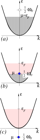
Figure 19: An illustration of the BCS-BEC crossover in the limit of a vanishing resonance width $\gamma_{s}\rightarrow 0$. The evolution with detuning $\omega_{0}$ is illustrated, with (a) the BCS regime of $\omega_{0}>2\epsilon_{F}$, where particles are all free atoms forming a Fermi sea, (b) the crossover regime of $0<\omega_{0}<2\epsilon_{F}$, where a fraction of atoms between $\omega_{0}$ and $\epsilon_{F}$ have converted into BEC of bosonic molecules, and (c) the BEC regime of $\omega_{0}<0$, where only Bose-condensed molecules are present.

For a large positive detuning $\omega_{0}>2\epsilon_{F}$, molecules are too energetically costly to be produced in equilibrium, and all particles are fermionic atoms forming a Fermi sea, with the chemical potential locked to the Fermi energy $\mu=\epsilon_{F}$, with

$$\epsilon_{F}={\left(3\pi^{2}n\right)^{2/3}\over 2m}.$$ (173)

set completely by the total particle density $n$. However, as illustrated in Fig. 19, for an intermediate range of detuning $\omega_{0}<2\epsilon_{F}$, it becomes energetically advantageous to convert a fraction of fermions in the Fermi sea between $\omega_{0}$ and $2\epsilon_{F}$ into Bose-condensed molecules, thereby keeping the effective bosonic chemical potential $2\mu-\omega_{0}$ at its lowest value of zero. This atom-to-molecule conversion regime continues as detuning is reduced, with $\mu$ locked to $\omega_{0}/2$. It terminates when $\omega_{0}$ reaches $0$, at which point atom-to-molecule conversion is complete and the system enters into the BEC regime of a pure molecular condensate for $\omega_{0}<0$. The full range of behavior can be summarized by the evolution of the molecular boson density, $n_{b}(\omega_{0})$ with detuning $\omega_{0}$, that can be easily found to be

$$n_{b} = \cases{0,\ &\text{for $\omega_{0}>2\epsilon_{F}$}\cr{n\over 2}\left(1-\left({\omega_{0}\over 2\epsilon_{F}}\right)^{3/2}\right),\ &\text{for $0\leq\omega_{0}\leq 2\epsilon_{F}$}\cr{n\over 2},\ &\text{for $\omega_{0}<0$}.}$$ (174)

and is displayed in Fig. 20.

Figure 20: The normalized density of bosonic molecules $\hat{n}_{b}=2n_{b}/n$ vs the normalized detuning $\hat{\omega}_{0}=\omega_{0}/\epsilon_{F}$ in the limit of a vanishing resonance width, $\gamma_{s}\rightarrow 0$ .

For finite temperature the chemical potential is no longer locked to the detuning and is determined by the particle number equation Eq. (171), together with the noninteracting expressions for the fermionic density

$$n_{f}=2\int{d^{3}k\over(2\pi)^{3}}{1\over e^{{k^{2}\over 2mT}-{\mu\over T}}+1},$$ (175)

and the bosonic density

$$n_{b}=\int{d^{3}k\over(2\pi)^{3}}{1\over e^{{k^{2}\over 4mT}-{2\mu-\omega_{0}\over T}}-1}+n_{0},$$ (176)

where $n_{0}=|B|^{2}$ is, as usual, the density of the bosonic condensate. This total number constraint must be supplemented by the free-energy minimization rule that $n_{0}>0$ only if $2\mu=\omega_{0}$ and vanishes otherwise.

These equations can then be used to determine the normal-superfluid transition temperature $T_{c}(\omega_{0})$, defined as a temperature at a given detuning $\omega_{0}$ at which $n_{0}$ first vanishes. Setting $2\mu=\omega_{0}$ and $n_{0}=0$, we find an implicit equation

$$\int{d^{3}k\over(2\pi)^{3}}{1\over e^{{k^{2}\over 2mT_{c}}-{\omega_{0}\over 2T_{c}}}+1}+\int{d^{3}k\over(2\pi)^{3}}{1\over e^{{k^{2}\over 4mT_{c}}}-1}={n\over 2},$$ (177)

that uniquely gives $T_{c}(\omega_{0})$. The numerical solution of Eq. (177) is presented in Fig. 21.

The limiting behavior of $T_{c}(\omega_{0})$ is easy to deduce. Deep in the BEC regime, for $\omega_{0}\ll-\epsilon_{F}$, the first integral is exponentially small, reflecting the fact that in this regime the fermion chemical potential $\mu$ is large and negative and a number of thermally created fermionic atoms is strongly suppressed. The second integral then gives the critical temperature, that in this regime coincides with the BEC transition temperature

$$T_{\rm c}(\omega_{0}\ll-\epsilon_{F})\approx T_{\rm BEC}={\pi\over m}\left({n\over 2\zeta\left({3/2}\right)}\right)^{2/3},$$ (178)

that is indeed on the order of $\epsilon_{F}$. As $\omega_{0}$ is increased through the BEC and crossover regimes, $T_{c}(\omega_{0})$ decreases, as the contribution of thermally created free atoms from the first integral increases. When detuning reaches $\omega_{0}=2\epsilon_{F}$, the solution of Eq. (177) drops down to $T_{c}(2\epsilon_{F})=0$. Beyond this point, for $\omega_{0}>2\epsilon_{F}$ in the BCS regime, the bosons are completely converted into free fermions forming a Fermi sea and $T_{c}(\omega_{0})$ sticks at $0$.

Figure 21: The normalized critical temperature $\hat{T}_{c}=T_{c}/T_{\rm BEC}$ as a function of the normalized detuning $\hat{\omega}_{0}=\omega_{0}/\epsilon_{F}$ in the limit of a vanishing resonance width $\gamma_{s}\rightarrow 0$.

VI.2 Narrow-resonance limit

We extend our study of the $s$-wave resonant Fermi gas, described by the Bose-Fermi mixture action to the limit where $\gamma_{s}$ is small but nonzero. The overall qualitative picture is quite similar to the $g_{s}\rightarrow 0$ limit discussed in the previous subsection and summarized in Fig.19, with only a few new features.

Because of the $\phi$ nonlinearities in $S_{s}[\phi]$, Eq. (170), the functional integral Eq. (169) in general cannot be evaluated exactly. However, as discussed in the Introduction and in Sec. V.1, for small $g_{s}$ ($\gamma_{s}\ll 1$) the theory can be analyzed by a controlled perturbative expansion in powers of $\gamma_{s}$ around the saddle-point (mean-field) approximation of $Z_{s}$. To this end, we look for the spatially uniform field configuration $\phi({\bf r})=B$ that minimizes the action $S_{s}\left[\phi\right]$. We find the following saddle-point equation

$${1\over B}\left.{\delta S_{s}\left[\phi\right]\over~{}\delta\bar{\phi}}\right|_{\phi=B}=$$

$$\epsilon_{0}-2\mu-g_{s}^{2}T\sum_{\omega_{n}}\int{d^{3}k\over(2\pi)^{3}}{1\over\omega_{n}^{2}+\left({k^{2}\over 2m}-\mu\right)^{2}+g_{s}^{2}\bar{B}B}=0.$$ (179)

where $\omega_{n}=\pi T(2n+1)$ are the fermion Matsubara frequencies. The sum over the frequencies can be done in a closed form, leading to the so-called BCS-BEC gap equation for the mean field $B(T,\mu,\epsilon_{0})$ (and the corresponding condensate density $|B|^{2}$)

$$\epsilon_{0}-2\mu={g_{s}^{2}\over 2}\int{d^{3}k\over(2\pi)^{3}}{\tanh\frac{E_{k}}{2T}\over E_{k}},$$ (180)

where $E_{k}$ is given by

$$E_{k}=\sqrt{\left({k^{2}\over 2m}-\mu\right)^{2}+g_{s}^{2}\bar{B}B}$$ (181)

The integral on the right hand side of the BCS-BEC gap equation is formally divergent, scaling linearly with the uv momentum cutoff $\Lambda$. However, expressing the bare detuning parameter $\epsilon_{0}$ in terms of the physical, renormalized detuning $\omega_{0}$ using Eq. (120), we can completely eliminate the appearance of the microscopic uv scale $\Lambda$ in all physical quantities, and thereby obtain a uv-convergent form of the BCS-BEC gap equation

$$\omega_{0}-2\mu={g_{s}^{2}\over 2}\int{d^{3}k\over(2\pi)^{3}}\left[{\tanh{E_{k}\over 2T}\over E_{k}}-{2m\over k^{2}}\right].$$ (182)

To calculate $Z_{s}$ in the saddle-point approximation, we write the bosonic field

$$\phi({\bf r})=B+\varphi({\bf r}),$$ (183)

in terms of a fluctuation field $\varphi({\bf r})$ about the saddle point $B$. Expanding the action, we find

$$S_{s}\left[B,\varphi\right]\approx S_{0}[B]+S_{\rm fluct}[B,\varphi],$$ (184)

where

$$S_{0}[B]=\left.S_{s}\right|_{\phi=B}={V\over T}\left(\epsilon_{0}-2\mu\right)\bar{B}B-V\sum_{\omega_{n}}\int{d^{3}k\over(2\pi)^{3}}\ln\left[\omega_{n}^{2}+\left({k^{2}\over 2m}-\mu\right)^{2}+g_{s}^{2}\bar{B}B,\right]$$ (185)

and

$$S_{\rm fluct}[B,\varphi]=\sum_{p,\Omega_{n}}\left(\matrix{\bar{\varphi}_{p,\Omega_{n}}&\varphi_{-p,-\Omega_{n}}}\right)\left(\matrix{\frac{1}{2}s_{B}(p,\Omega_{n})+\Sigma_{11}\left(p,\Omega_{n}\right)&\Sigma_{20}\left(p,\Omega_{n}\right)\cr\Sigma_{20}(p,\Omega_{n})&\frac{1}{2}s_{B}(p,-\Omega_{n})+\Sigma_{11}\left(p,-\Omega_{n}\right)}\right)\left(\matrix{\varphi_{p,\Omega_{n}}\cr\bar{\varphi}_{-p,-\Omega_{n}}}\right).$$ (186)

Here $s_{B}(p,\Omega_{n})=i\Omega_{n}+\epsilon_{0}-2\mu+{p^{2}\over 4m}$ represents the free part of the bosonic action, $\Sigma_{11}(p,\omega)$ and $\Sigma_{02}(p,\omega)$ are the normal and anomalous fermion polarization operators, and $\Omega_{n}=2\pi Tn$ are the bosonic Matsubara frequencies. We used here a fact that $\Sigma_{20}$ is symmetric under the sign change of its arguments. The explicit expressions for the polarization operators are not very illuminating at this stage and will be discussed later (see Eqs. (237) and (238)). Within this saddle-point approximation, the partition function $Z_{s}$ is given by

$$Z_{s}\approx\exp\left(-S_{0}\right)\int{\cal D}\varphi{\cal D}\bar{\varphi}\exp\left(-S_{\rm fluct}\right).$$ (187)

In the applications of Eq. (180) to atomic gases, it is the total particle number $N$, rather than the chemical potential that is controlled experimentally. Of course, as usual, in the thermodynamic limit there is no distinction between the two ensembles and it is sufficient to work in the grand-canonical ensemble (as we have done above), and then eliminate $\mu$ in favor of $N$ through the particle number equation

$$N=T\frac{\partial}{\partial\mu}\ln Z_{s}.$$ (188)

Solving (188) simultaneously with the BCS-BEC gap equation (182) determines the condensate density $B$ and chemical potential $\mu$ as a function of experimentally controlled parameters, the detuning $\omega_{0}$, temperature $T$, and particle number $N$.

VI.2.1 Zero temperature BCS-BEC crossover

At zero temperature the BCS-BEC gap equation reduces to

$$\omega_{0}-2\mu={g_{s}^{2}\over 2}\int{d^{3}k\over(2\pi)^{3}}\left[{1\over E_{k}}-{2m\over k^{2}}\right].$$ (189)

The particle number equation can also be evaluated noting that at $T=0$ and small $\gamma_{s}$, most of the weakly-interacting bosons remain in the condensate $B$ (with only a small interaction-driven depletion set by $\gamma_{s}$) and therefore the fluctuations $\varphi({\bf r})$ are small and can be safely neglected. Omitting $S_{\rm fluct}$ from $Z_{s}$ above and using Eq. (185), the particle number-density ($n=N/V$) equation is then given by

$$n = -{T\over V}\frac{\partial S_{0}}{\partial\mu},$$ (190)

$$= \int{d^{3}k\over(2\pi)^{3}}\left[1-{\xi_{k}\over E_{k}}\right]+2\bar{B}B,$$

where $E_{k}$ is still given by Eq. (181), and

$$\xi_{k}={k^{2}\over 2m}-\mu.$$ (191)

Before solving this equation together with the BCS-BEC gap equation, (189) for the condensate $B$ and the chemical potential $\mu$ as a function of $\omega_{0}$, let us comment on the nature of the ground state. The bosons, within the narrow resonance approximation, where the condensate depletion has been neglected, are all located in the condensate. The fermions, on the other hand, form a paired superfluid described by the BCS-like Hamiltonian

$$H-\mu~{}N_{f}=\sum_{{\bf k},\sigma}\xi_{k}~{}\hat{a}^{\dagger}_{{\bf k}\sigma}\hat{a}_{{\bf k}\sigma}+$$

$$\sum_{{\bf k}}~{}g_{s}\left(B~{}\hat{a}^{\dagger}_{{\bf k}\uparrow}\hat{a}^{\dagger}_{-{\bf k}\downarrow}+\bar{B}~{}\hat{a}_{-{\bf k}\downarrow}\hat{a}_{{\bf k}\uparrow}\right),$$ (192)

with the condensate $B$ appearing as pairing parameter to be self-consistently determined. In practice, $B$ can always be chosen to be real due to the symmetry $B\rightarrow e^{i\varphi}B$, so that $B=\bar{B}$. The role of the BCS gap is played by the bosonic density, via

$$\Delta=g_{s}B.$$ (193)

The ground state of this Hamiltonian is the BCS wavefunction Schrieffer (1989)

$$\left|{\rm BCS}\right\rangle=\prod_{k}\left(u_{k}+v_{k}~{}a^{\dagger}_{k\uparrow}a^{\dagger}_{-k\downarrow}\right)\left|0\right\rangle,$$ (194)

with $u_{k}$, $v_{k}$ given by the standard expressions

$$v_{k}=\sqrt{\frac{1}{2}\left(1-{\xi_{k}\over E_{k}}\right)},\ u_{k}=\sqrt{\frac{1}{2}\left(1+{\xi_{k}\over E_{k}}\right)}.$$ (195)

When $\omega_{0}$ is large and positive, $\omega_{0}\gtrsim 2\epsilon_{F}$, the closed-channel molecules (bosons $\hat{b}_{\bf p}$) are energetically suppressed and Eq. (VI.2.1) predicts phenomenology of a BCS superconductor Schrieffer (1989). Namely, most of the particles will be fermionic atoms with a weak attraction due to exchange of virtual bosons (resonances) with energy detuned much higher than the chemical potential. Such degenerate fermions will therefore form a BCS ground state (194). Due to fermionic pairing, the bosons will still be present, albeit in the exponentially small numbers since the BCS gap Eq. (193) and the associated Cooper-pair density are exponentially small.

In a qualitative picture similar to the $g_{s}\rightarrow 0$ limit (see Fig. 19), as $\omega_{0}$ is decreased the number of boson condensate will grow, while the number of fermions will decrease, with the substantial change approximately (within a window $\gamma_{s}\epsilon_{F}$) taking place when $\omega_{0}$ drops below $2\epsilon_{F}$. As $\omega_{0}$ crosses $0$, the chemical potential that tracks it for $\omega_{0}<2\epsilon_{F}$ will also change sign and become negative. At this point the remaining fermions will form a “strongly-coupled superconductor” (in the notation of Ref. Read and Green (2000)) that exhibits pairing in the absence of a Fermi surface, driven by the existence of a true two-body bound state. Such situation is not typically encountered nor experimentally accessible in ordinary, solid-state superconductors. As discussed in Ref. Read and Green (2000), a strongly coupled $s$-wave superconductor is not qualitatively different from the more standard one with $\mu>0$. This contrasts with the $p$-wave case, where $\mu>0$ and $\mu<0$ regimes are separated by a (possibly topological) quantum phase transition, that we will discussed in Sec. VII devoted to $p$-wave resonances. Because throughout the entire range of detuning $\omega_{0}$ (particularly for $0<\omega_{0}<2\epsilon_{F}$) the system will be a superposition of Bose-condensed bosons and Cooper-paired fermions, we refer to it as a BCS-BEC condensate.

It is useful to contrast this small $\gamma_{s}$ picture of BCS-BEC condensate with the earlier studies of wide resonances (corresponding to the large $\gamma_{s}$ limit in our setting). When the resonance is wide, most of the particles are fermions regardless of the value of $\omega_{0}$ (open-channel fermions in the atomic physics parlance) and only a small fraction of the condensate will be bosons (closed-channel fermions). As a result, for a wide resonance no sharp features exist in the BCS-BEC crossover.

Now we are in the position to solve the BCS-BEC gap and the particle number equations. The former can be written as

$$\omega_{0}-2\mu={g_{s}^{2}\left(2m\right)^{3\over 2}\sqrt{|\mu|}\over 4\pi^{2}}~{}I\left(u\right),$$ (196)

where $u={g_{s}B/\mu}$ (with $B=\bar{B}$), and the integral $I(u)$ is given by

$$I(u)=\int_{0}^{\infty}dx~{}\left[{x^{2}\over\sqrt{\left(x^{2}-{\rm sign}~{}u\right)^{2}+u^{2}}}-1\right],$$ (197)

with ${\rm sign}~{}u={\rm sign}~{}\mu$. Similarly, the particle number equation reduces to

$${(2m)^{3\over 2}|\mu|^{3\over 2}\over 3\pi^{2}}K(u)+2B^{2}=N,$$ (198)

where $K(u)$ is defined as

$$K(u)={3\over 2}\int_{0}^{\infty}dx~{}x^{2}\left[1-{x^{2}-{\rm sign}~{}u\over\sqrt{(x^{2}-{\rm sign}~{}u)^{2}+u^{2}}}\right].$$ (199)

$K(u)$ essentially measures the deviation of the particle number from the usual Fermi distribution in the absence of pairing, with $K(u\rightarrow 0^{+})\rightarrow 1$.

In the BCS regime we expect a small condensate with $u\ll 1$, for which

$$I(u)\approx\ln\left(8\over e^{2}u\right).$$ (200)

The logarithmic divergence of $I(u)$ as $u$ goes to zero is the standard Fermi surface contribution to the gap equation. In the same regime we can replace $K(u)$ by $K(0^{+})=1$. We thus find

$$B\approx g_{s}^{-1}8e^{-2}\mu\exp\left(-{4\pi^{2}\left(\omega_{0}-2\mu\right)\over(2m)^{3/2}g_{s}^{2}\sqrt{\mu}}\right),$$ (201)

and

$${(2m\mu)^{3/2}\over 3\pi^{2}}+2B^{2}=n.$$ (202)

Since $B$ is exponentially small, Eq. (202) gives $\mu\approx\epsilon_{F}$. Combined, these two equations give us $B(\omega_{0})$ as a function of detuning. The quantitative validity of this regime, $u\ll 1$ is given by

$$\omega_{0}\gg 2\epsilon_{F}+\epsilon_{F}\gamma_{s},$$ (203)

where $\gamma_{s}$ is the small parameter given by Eq. (123) characterizing an $s$-wave resonant gas at density $n$.

As $\omega_{0}$ is decreased below $2\epsilon_{F}$, a crossover regime is entered as fermions begin to be converted into bosons, and the chemical potential $\mu$ tracks $\omega_{0}/2$ to accuracy ${\cal O}(\gamma_{s})$. As is clear from the infinitely narrow resonance analysis, Eq. (174) and Fig.19, most of the atoms will pair up into bosons that become true bound states inside the BEC regime of $\omega_{0}<0$. In this BEC regime, for a sufficiently negative $\omega_{0}$, so that $u<0$ and $|u|\ll 1$, we can use the following simple asymptotics $I(-0)=-{\pi\over 2}$, and $K(u)\approx{3\pi\over 16}u^{2}$, to reduce the gap and particle number equations deep in the BEC regime to be

$$\omega_{0}-2\mu \approx -{g_{s}^{2}(2m)^{3/2}\sqrt{|\mu|}\over 8\pi},$$ (204)

$$n \approx {(2m)^{3/2}g_{s}^{2}B^{2}\over 16\pi\sqrt{|\mu|}}+2B^{2}.$$ (205)

These give a BCS-BEC condensate, in which most particles are molecular (true bound states) bosons, and only a small fraction of the total number are the Cooper-paired fermions.

The full solution of Eqs. (196) and (198) can only be found numerically and is displayed in Fig. 6 for $\gamma=0.1$. We can see that in contrast of the infinitely narrow resonance case presented earlier on Fig. 20, the molecular condensate density $n_{b}=B^{2}$ extends to $\epsilon_{0}\geq 2\epsilon_{F}$, although only as an exponentially small tail. This represents the BCS condensate absent in the limit of an infinitely narrow resonance, $\gamma_{s}\rightarrow 0$.

VI.2.2 Ground state energy across BCS-BEC crossover

It is instructive to also calculate the zero temperature grand canonical ground-state energy density $\varepsilon_{GS}(\mu,\omega_{0},B)$, that is given by the $T\rightarrow 0$ limit of $TS_{0}/V$, where $S_{0}$ is given by Eq. (185). Calculating it at arbitrary $B$ and then minimizing it with respect to $B$ will be of course be equivalent to solving the gap equation Eq. (189). As in the previous subsection, to lowest order in $\gamma_{s}$, ignoring quantum fluctuations of $\phi$, we find

$$\varepsilon_{GS}=(\omega_{0}-2\mu)B^{2}+\sum_{k}(\xi_{k}-E_{k}+g_{s}^{2}\frac{B^{2}}{2\epsilon_{k}}).$$ (206)

Here we again chose $B$ to be real, traded $\epsilon_{0}$ for $\omega_{0}$, and used the notations Eqs. (191), (181) with the additional notation

$$\epsilon_{k}=\frac{k^{2}}{2m}.$$ (207)

Setting $B=0$ the normal state energy is easily computed as

$$\varepsilon_{GS}(B=0) = \sum_{k}(\xi_{k}-|\xi_{k}|),$$ (208)

$$= -\frac{8}{15}c\mu^{5/2}\Theta(\mu),$$ (209)

where we converted the sum to an integral and used the three-dimensional density of states $N(E)=c\sqrt{E}$ with

$$c\equiv\frac{m^{3/2}}{\sqrt{2}{\pi^{2}}}.$$ (210)

Combining this with Eq. (206) then gives:

$$\varepsilon_{GS}=(\omega_{0}-2\mu)B^{2}-\frac{8}{15}c\mu^{5/2}\Theta(\mu)+J(\mu,B),$$ (211)

where

$$J(\mu,B)\equiv\int\frac{d^{3}k}{(2\pi)^{3}}\big{(}|\xi_{k}|-E_{k}+g_{s}^{2}\frac{B^{2}}{2\epsilon_{k}}\big{)},$$ (212)

and we have converted the momentum sum to an integral.

The gap equation discussed previously, Eq. (189), and the particle number equation Eq. (190) obviously follow from

$$0=\frac{\partial\varepsilon_{GS}}{\partial B},$$ (213)

and

$$n=-\frac{\partial\varepsilon_{GS}}{\partial\mu}.$$ (214)

For a narrow Feshbach resonance ($\gamma_{s}\ll 1$), we can find an accurate analytic approximations to $\varepsilon_{GS}$ in Eq. (211) in all relevant regimes. The first step is to find an appropriate approximation to Eq. (212), which has drastically different properties depending on whether $\mu>0$ (so that the low-energy states are near the Fermi surface) or $\mu<0$ (so that there is no Fermi surface and excitations are gapped with energy bounded from below by $|\mu|$). We proceed by first evaluating the derivative $\frac{\partial J}{\partial B}$ and then integrating the expression with a constant of integration $J(\mu,0)=0$.

$$\frac{\partial J}{\partial B}=-g_{s}^{2}B\int\frac{d^{3}k}{(2\pi)^{3}}\big{(}\frac{1}{E_{k}}-\frac{1}{\epsilon_{k}}\big{)},$$ (215)

$$\quad\,\,\,\,\,=-g_{s}^{2}B\int_{0}^{\infty}\sqrt{\epsilon}d\epsilon\big{(}\frac{1}{\sqrt{(\epsilon-\mu)^{2}+\Delta^{2}}}-\frac{1}{\epsilon}\big{)},$$ (216)

$$\quad\,\,\,\,\,\simeq-2g_{s}^{2}N(\mu)B\ln\frac{8{\rm e}^{-2}\mu}{g_{s}B},\hskip 2.84544pt\mu>0;\mu\gg g_{s}B,$$ (217)

$$\quad\,\,\,\,\,\simeq g_{s}^{2}N(\mu)B\Big{[}\pi+\frac{\pi}{16}\big{(}\frac{g_{s}B}{\mu}\big{)}^{2}\Big{]},\mu\ll-g_{s}B,$$ (218)

This calculation proceeds through the evaluation of the integral for $I(u)$, Eq. (197). Integrating back up with respect to $B$, we thus have

$$J\simeq\cases{-N(\mu)\big{(}\frac{g_{s}^{2}B^{2}}{2}+g_{s}^{2}B^{2}\ln\frac{8{\rm e}^{-2}\mu}{g_{s}B}\big{)},\ &\text{$\mu>0$; $\mu\gg g_{s}B$},\cr N(\mu)\frac{g_{s}^{2}B^{2}}{2}\Big{[}\pi+\frac{\pi}{32}\big{(}\frac{g_{s}B}{\mu}\big{)}^{2}\Big{]},\ &\text{$\mu<0$; $|\mu|\gg g_{s}B$},\cr}$$

Having computed $\varepsilon_{GS}(\mu,B)$ in the regimes of interest, the phase diagram is easily deduced by finding $B$ that minimizes $\varepsilon_{GS}(\mu,B)$, subject to the total atom number constraint Eq. (214).

BCS regime:

The BCS regime is defined by $\omega_{0}\gg 2\epsilon_{\rm F}$, where $g_{s}B\ll\mu$ and $\mu\simeq\epsilon_{\rm F}>0$, with pairing taking place in a thin shell around the well-formed Fermi surface. In this regime, $\varepsilon_{GS}$ is given by

$$\varepsilon_{GS}\simeq-c\frac{\sqrt{\mu}}{2}\Delta^{2}+\frac{\Delta^{2}}{g_{s}^{2}}(\delta-2\mu)+c\sqrt{\mu}\Delta^{2}\ln\frac{\Delta}{8{\rm e}^{-2}\mu}$$

$$\qquad\qquad-\frac{8}{15}c\mu^{5/2}$$ (220)

with $\Delta\equiv g_{s}B$, see Eq. (193).

It is convenient to work with the dimensionless variables defined by

$$\hat{\mu}=\frac{\mu}{\epsilon_{F}},\ \hat{\Delta}=\frac{\Delta}{\epsilon_{F}},\ \hat{\omega}_{0}=\frac{\omega_{0}}{\epsilon_{F}}.$$ (221)

The normalized ground-state energy $e_{GS}$ in the BCS regime is then given by

$$e_{GS}\equiv\frac{\varepsilon_{GS}}{c\epsilon_{\rm F}^{5/2}}\simeq-\frac{\sqrt{\hat{\mu}}}{2}\hat{\Delta}^{2}+\hat{\Delta}^{2}(\hat{\omega}_{0}-2\hat{\mu})\gamma_{s}^{-1}$$

$$\qquad+\sqrt{\hat{\mu}}\hat{\Delta}^{2}\ln\frac{\hat{\Delta}}{8{\rm e}^{-2}\hat{\mu}}-\frac{8}{15}\hat{\mu}^{5/2},$$ (222)

where, $\gamma_{s}$, defined in Eq. (123), is a dimensionless measure of the Feshbach resonance width $0pt$ to the Fermi energy. With this, Eqs. (213) and (214) become

$$0=\frac{\partial e_{GS}}{\partial\hat{\Delta}},$$ (223)

$$\quad\simeq 2\hat{\Delta}(\hat{\omega}_{0}-2\hat{\mu})\gamma_{s}^{-1}+2\sqrt{\hat{\mu}}\hat{\Delta}\ln\frac{\hat{\Delta}}{8{\rm e}^{-2}\hat{\mu}},$$ (224)

$$\frac{4}{3}=-\frac{\partial e_{GS}}{\partial\hat{\mu}},$$ (225)

$$\quad\simeq\frac{5}{4}\frac{\hat{\Delta}^{2}}{\sqrt{\hat{\mu}}}+\frac{4}{3}\hat{\mu}^{3/2}+2\hat{\Delta}^{2}\gamma_{s}^{-1}-\frac{\hat{\Delta}^{2}}{2\sqrt{\hat{\mu}}}\ln\frac{\hat{\Delta}}{8{\rm e}^{-2}\hat{\mu}},$$ (226)

that admits the normal state ($\hat{\Delta}=0$, $\hat{\mu}=1$) and the BCS SF state

$$\hat{\Delta} \simeq \hat{\Delta}_{\rm BCS}(\hat{\mu})\equiv 8{\rm e}^{-2}\hat{\mu}{\rm e}^{-\gamma_{s}^{-1}(\hat{\omega}_{0}-2\hat{\mu})/\sqrt{\hat{\mu}}},$$ (227)

$$\frac{4}{3} \simeq \frac{4}{3}\hat{\mu}^{3/2}+2\hat{\Delta}^{2}\gamma_{s}^{-1}.$$ (228)

where in the second line we approximately neglected the first term on the right side of Eq. (226), valid since $\hat{\Delta}_{\rm BCS}\ll 1$ (and $\gamma_{s}\ll 1$). It is easy to show that the BCS solution is always a minimum of $\varepsilon_{GS}(B)$.

The meaning of the two terms on the right side of Eq. (228) is clear once we recall its form in terms of dimensionful quantities:

$$n\simeq\frac{4}{3}c\mu^{3/2}+2|B|^{2},$$ (229)

i.e., the first term simply represents the total unpaired atom density, reduced below $n$ since $\mu<\epsilon_{\rm F}$, while the second term represents the density of atoms bound into molecules, i.e., twice the molecular condensate density $|B|^{2}$. Qualitatively, we see that at large $\hat{\omega}_{0}$, $\hat{\Delta}\ll 1$, implying from the number equation that $\hat{\mu}\approx 1$.

BEC regime:

We next consider the BEC regime defined by $\omega_{0}<0$. As we shall see, in this regime $\mu<0$ and $|\mu|\gg\Delta$, so that Eq. (VI.2.2), $I(\mu,\Delta)$, applies. This yields, for the normalized ground-state energy,

$$e_{G}\simeq(\hat{\omega}_{0}-2\hat{\mu})\hat{\Delta}^{2}\gamma_{s}^{-1}+\sqrt{|\hat{\mu}|}\frac{\hat{\Delta}^{2}}{2}\Big{[}\pi+\frac{\pi}{32}\big{(}\frac{\hat{\Delta}}{\hat{\mu}}\big{)}^{2}\Big{]},$$ (230)

and, for the gap and number equations (dividing by an overall factor of $\hat{\Delta}$ in the former)

$$0 \simeq 2\gamma_{s}^{-1}(\hat{\omega}_{0}-2\hat{\mu})+\sqrt{|\hat{\mu}|}\Big{[}\pi+\frac{\pi}{16}\big{(}\frac{\hat{\Delta}}{\hat{\mu}}\big{)}^{2}\Big{]},$$ (231)

$$\frac{4}{3} \simeq 2\gamma_{s}^{-1}\hat{\Delta}^{2}+\frac{\hat{\Delta}^{2}\pi}{4\sqrt{|\hat{\mu}|}}.$$ (232)

In the BEC regime the roles of the two equations are reversed, with $\hat{\mu}$ approximately determined by the gap equation and $\hat{\Delta}$ approximately determined by the number equation. Thus, $\hat{\mu}$ is well-approximated by neglecting the term proportional to $\hat{\Delta}^{2}$ in Eq. (231), giving

$$\hat{\mu} \approx \frac{\hat{\omega}_{0}}{2}\Big{[}\sqrt{1+\frac{\gamma_{s}^{2}\pi^{2}}{32|\hat{\omega}_{0}|}}-\frac{\gamma_{s}\pi}{\sqrt{32|\hat{\omega}_{0}|}}\Big{]}^{2}.$$ (233)

At large negative detuning, $|\hat{\omega}_{0}|\gg 1$, in other words in the BEC regime, Eq. (233) reduces to $\hat{\mu}\approx\hat{\omega}_{0}/2$, with the chemical potential tracking the detuning.

Inserting Eq. (233) into Eq. (232) yields

$$\hat{\Delta}^{2}=\frac{2\gamma_{s}}{3}\Big{[}1-\frac{\gamma_{s}\pi}{\sqrt{(\gamma_{s}\pi)^{2}+32|\hat{\omega}_{0}|}}\Big{]}.$$ (234)

Using $\hat{\Delta}=\Delta/\epsilon_{\rm F}$ and the relation $\Delta^{2}=g_{s}^{2}n_{b}$ between $\Delta$ and the molecular density, we have

$$n_{b} = \frac{3}{4}\gamma_{s}^{-1}\hat{\Delta}^{2}n,$$ (235)

$$\simeq \frac{n}{2}\Big{[}1-\frac{\gamma_{s}\pi}{\sqrt{(\gamma_{s}\pi)^{2}+32|\hat{\omega}_{0}|}}\Big{]},$$ (236)

which, as expected (given the fermions are nearly absent for $\mu<0$) simply yields $n_{b}\approx n/2$ in the asymptotic (large $|\hat{\omega}_{0}|$) BEC regime.

These results of course match those derived purely on the basis of the gap and particle number equations in Sec. VI.2.1.

VI.2.3 Zero temperature collective excitations and condensate depletion

We would now like to calculate the spectrum of collective excitations of the BEC-BCS condensate, which is contained in the $S_{\rm fluct}$ part of the effective action. In order to do that, we need expressions for the self-energies $\Sigma_{11}$ and $\Sigma_{20}$ appearing in Eq. (186). At zero temperature these are given by

$$\Sigma_{11}\left(q,\Omega\right)={g_{s}^{2}\over 2}\int{d\omega\over 2\pi}{d^{3}k\over(2\pi)^{3}}\frac{\left[i\left({\Omega\over 2}+\omega\right)-\xi_{+}\right]\left[i\left(\omega-{\Omega\over 2}\right)+\xi_{-}\right]}{\left[\left({\Omega\over 2}+\omega\right)^{2}+\xi_{+}^{2}+g_{s}^{2}B^{2}\right]\left[\left(\omega-{\Omega\over 2}\right)^{2}+\xi_{-}^{2}+g_{s}^{2}B^{2}\right]},$$ (237)

and

$$\Sigma_{20}\left(q,\Omega,\right)={g_{s}^{4}B^{2}\over 2}\int{d\omega\over 2\pi}{d^{3}k\over(2\pi)^{3}}\frac{1}{{\left[\left({\Omega\over 2}+\omega\right)^{2}+\xi_{+}^{2}+g_{s}^{2}B^{2}\right]\left[\left(\omega-{\Omega\over 2}\right)^{2}+\xi_{-}^{2}+g_{s}^{2}B^{2}\right]}},$$ (238)

where

$$\xi_{+}={1\over 2m}\left({\bf k}+{{\bf q}\over 2}\right)^{2}-\mu,\ \xi_{-}={1\over 2m}\left({\bf k}-{{\bf q}\over 2}\right)^{2}-\mu.$$ (239)

The self-energy $\Sigma_{11}$ involves an IR divergent integral over $k$. This divergence can be regularized if one notices that $\Sigma_{11}$ enters the effective action $S_{\rm fluct}$ in the combination $\epsilon_{0}-2\mu+2\Sigma_{11}$. It is straightforward to check, however, that

$$\epsilon_{0}-2\mu+2\Sigma_{11}(0,0)=2\Sigma_{20}(0,0),$$ (240)

by virtue of the saddle-point equation Eq. (189). This situation is typical in the interacting Bose gas, and Eq. (240) is nothing but the Goldstone theorem ensuring that the collective excitations remain massless (also referred to as Hugenholtz-Pines relation Hugenholtz and Pines (1959) in the interacting Bose gas literature). Therefore, we are really interested not in $\Sigma_{11}(q,\Omega)$, but rather in the linear combination $\Sigma_{11}(q,\Omega)-\Sigma_{11}(0,0)$, which remains finite.

The spectrum of collective excitations is given by the condition that the propagator computed with the help of Eq. (186) has a pole. To simply the calculations, we will only compute the spectrum at low momentum and energy. Following Levitov and Barankov (2004), in anticipation that the collective excitations are sound waves and so, $\Omega_{q}\sim q$, we expand the self-energies in powers of energy and momentum according to

$$\epsilon_{0}-2\mu+2\Sigma_{11}(q,\Omega) \approx 2\Sigma_{0}+\Sigma i\Omega+\Sigma_{1}\Omega^{2}+\Pi_{1}q^{2}$$

$$\Sigma_{20}(q,\Omega) \approx \Sigma_{0}+\Sigma_{2}\Omega^{2}+\Pi_{2}q^{2}$$ (241)

where we have used Eq. (240). Therefore, the spectrum is given by the condition that the determinant of the matrix in Eq. (186) vanishes. That matrix in our case takes the form

$$\det\left(\matrix{\frac{1}{2}\left(i\Omega\left(1+\Sigma\right)+\frac{q^{2}}{4m}+2\Sigma_{0}+\Sigma_{1}\Omega^{2}+\Pi_{1}q^{2}\right)&\Sigma_{0}+\Sigma_{2}\Omega^{2}+\Pi_{2}\Omega^{2}\cr\Sigma_{0}+\Sigma_{2}\Omega^{2}+\Pi_{2}\Omega^{2}&\frac{1}{2}\left(-i\Omega\left(1+\Sigma\right)+\frac{q^{2}}{4m}+2\Sigma_{0}+\Sigma_{1}\Omega^{2}+\Pi_{1}q^{2}\right)}\right)=0.$$ (242)

This gives for the spectrum $\Omega_{q}$ of excitations

$$\Omega_{q}^{2}=q^{2}\frac{4\Sigma_{0}\left(\frac{1}{4m}+\tilde{\Pi}\right)}{\left(1+\Sigma\right)^{2}+4\Sigma_{0}\tilde{\Sigma}},$$ (243)

where we introduced the notation

$$\tilde{\Pi}=\Pi_{1}-2\Pi_{2},\ \tilde{\Sigma}=\Sigma_{1}-2\Sigma_{2}.$$ (244)

In other words, the excitations are indeed sound modes, with the speed of sound

$$c=\sqrt{\frac{4\Sigma_{0}\left(\frac{1}{4m}+\tilde{\Pi}\right)}{\left(1+\Sigma\right)^{2}+4\Sigma_{0}\tilde{\Sigma}}}.$$ (245)

We now evaluate $\Sigma_{0}$, $\Sigma$, $\tilde{\Pi}$, and $\tilde{\Sigma}$. Doing the frequency integral in $\Sigma_{2,0}(0,0)$ gives

$$\Sigma_{0}={g_{s}^{4}B^{2}\over 8}\int_{0}^{\infty}{k^{2}dk\over 2\pi^{2}}{1\over\left[\left({k^{2}\over 2m}-\mu\right)^{2}+g_{s}^{2}B^{2}\right]^{3/2}},$$ (246)

Differentiating $\Sigma_{11}(0,\Omega)$ with respect to $\Omega$ at $\Omega=0$ gives

$$\Sigma={g_{s}^{2}\over 4}\int_{0}^{\infty}{k^{2}dk\over 2\pi^{2}}{{k^{2}\over 2m}-\mu\over\left[\left({k^{2}\over 2m}-\mu\right)^{2}+g_{s}^{2}B^{2}\right]^{3/2}}.$$ (247)

Finally, we also find after some algebra

$$\tilde{\Sigma}=\frac{g_{s}^{2}}{8}\int_{0}^{\infty}{k^{2}dk\over 2\pi^{2}}{1\over\left[\left({k^{2}\over 2m}-\mu\right)^{2}+g_{s}^{2}B^{2}\right]^{3/2}},$$ (248)

$$\tilde{\Pi}=\frac{\Sigma}{4m}+\frac{g_{s}^{4}B^{2}}{8m}\int_{0}^{\infty}{k^{2}dk\over 2\pi^{2}}\frac{\frac{k^{2}}{2m}}{\left(\left(\frac{k^{2}}{2m}-\mu\right)^{2}+g_{s}^{2}B^{2}\right)^{5/2}}.$$ (249)

In general, evaluation of the integrals in Eqs. (246), (247), (248), and (249) is straightforward but cumbersome. We will present results only in the deep BEC and BCS regimes (that is, $\omega_{0}\lesssim-\epsilon_{F}$ and $\omega_{0}\gtrsim\epsilon_{F}$).

First, consider the BEC side of the crossover. There $\omega_{0}$ and $\mu$ are negative, and it is clear that at small $g_{s}$, $\Sigma\ll 1$, $\Sigma_{0}\tilde{\Sigma}\ll 1$, and $m\tilde{\Pi}\ll 1$, and thus they can be neglected. The speed of sound is then simply given by

$$c_{\rm BEC}=\sqrt{\frac{\Sigma_{0}}{m}}.$$ (250)

Since $|\mu|\gg g_{s}^{2}B^{2}$ in this BEC regime, we can neglect $g_{s}^{2}B^{2}$ in the denominator of Eq. (246) to find

$$\Sigma_{0}\approx{g_{s}^{2}B^{2}\over 8}\int{k^{2}dk\over 2\pi^{2}}{1\over\left(\frac{k^{2}}{2m}-\mu\right)^{3}}={g_{s}^{4}B^{2}m^{3/2}\over 32\pi|\omega_{0}|^{3/2}},$$ (251)

where we have used $2\mu=\omega_{0}$ in this BEC regime. Therefore, the square of the speed of sound is simply

$$c^{2}_{\rm BEC}={g_{s}^{4}B^{2}m^{1/2}\over 32\pi|\omega_{0}|^{3/2}}.$$ (252)

where $B^{2}\approx{n/2}$. We compare this expression for $c^{2}_{\rm BEC}$ with a standard expression for a BEC condensates of point bosons (see, for example, Ref. Lifshitz and Pitaevskii (1980))

$$c^{2}={4\pi a_{b}B^{2}\over(2m)^{2}},$$ (253)

where $a_{b}$ is the boson scattering length (not to be confused with the scattering length of fermions, given by $a$ in Eq. (117)). By inspection, we therefore conclude that on the BEC side of the crossover, the BCS-BEC paired condensates behaves as an effective gas of weakly repulsive bosons with a scattering length

$$a_{b}={g_{s}^{4}m^{5/2}\over 32\pi^{2}|\omega_{0}|^{3/2}}.$$ (254)

We note that the scattering length $a_{b}$, together with the speed of sound $c$, decreases as the detuning $\omega_{0}$ is made more negative, deeper into the BEC regime. This is of course to be expected, as paired-bosons interaction arises due to their polarization into their constituent fermions, followed by a fermions exchange – the process of the order of $g_{s}^{4}$. Since this virtual fermion creation process costs a molecular binding energy, Eq. (36), deep in the BEC regime approximately given by $|\omega_{0}|$, it is suppressed with increasing $|\omega_{0}|$, as is the effective bosonic interaction and $a_{b}$.

Here an important remark is in order. Our narrow resonance result for $a_{b}$, Eq. (254), contrasts sharply with the well-known ($g_{s}$ and $m$ independent) result for the molecular scattering length deep in the BEC regime, namely $a_{b}\approx 0.6~{}a$, where $a$ is the fermion scattering length Petrov et al. (2005). The short answer explaining this difference is that the $a_{b}\approx 0.6~{}a$ prediction is for the wide resonance BEC regime, corresponding to $\gamma_{s}\rightarrow\infty$ instead of the limit of narrow resonance considered here. In more detail, the results of Ref. Petrov et al. (2005) apply only in the regime where $a\gg|r_{0}|$. In our narrow resonance problem, this regime is realized only in a very narrow range of $\omega_{0}$, satisfying $-\Gamma_{0}\lesssim\omega_{0}<0$ ($\Gamma_{0}$ is the resonance width given in Eq. (119)). This is not what one should call the BEC regime of the narrow resonance crossover, which should be defined as $\omega_{0}\lesssim-\epsilon_{F}$, with $\epsilon_{F}$, in turn, being much bigger than $\Gamma_{0}$.

Moreover, if one does tune $\omega_{0}$ to this narrow window, the Fermi energy of the gas under study here will be much bigger than the binding energy of the bosonic molecules, and the condensate cannot be treated at all as weakly interacting bosons. So even though the scattering length of bosons within this window of $\omega_{0}$ is indeed $0.6~{}a$, this will not get reflected in the speed of sound in the condensate.

Contrast this with the BEC regime of the broad resonance BCS-BEC superfluid, where $a\gg r_{0}$ for a wide range of the detuning $\omega_{0}<0$, and where Fermi energy is small compared to $\Gamma_{0}$. For further details, including the calculation of the speed of sound in the broad resonance BEC regime of Eq. (110), see Ref. Levinsen and Gurarie (2006).

Thus we conclude that Eq. (254) is the correct scattering length of molecules in the narrow resonance problem. In fact, Eq. (254) can also be derived independently by studying the scattering of bosons in vacuum perturbatively. We will not do it here.

Let us now turn to the BCS regime $\omega_{0}>2\epsilon_{F}$, where $\mu\approx\epsilon_{F}$. We evaluate $\Sigma_{0}$, $\Sigma$, $\tilde{\Sigma}$, and $\tilde{\Pi}$, from Eqs. (246), (247), and (248), (249). These integrals are easiest to compute if we change variables $k^{2}/(2m)-\mu=\xi$, and notice that only small $\xi$ essentially contribute to the integrals. We find

$$\Sigma_{0} \approx {g_{s}^{2}(2m)^{3/2}\over 16\pi^{2}}\mu^{1/2},\ \Sigma\approx{\omega_{0}-2\mu\over 4\mu},$$ (255)

$$\tilde{\Pi} \approx \frac{\mu\sqrt{(2m)^{3}\mu}}{24mB^{2}\pi^{2}},\ \tilde{\Sigma}\approx\frac{\sqrt{(2m)^{3}\mu}}{16B^{2}\pi^{2}}.$$ (256)

The speed of sound, Eq. (245), is now dominated by $\tilde{\Sigma}$, $\tilde{\Pi}$, and give

$$c_{\rm BCS}=\sqrt{\frac{\tilde{\Pi}}{\tilde{\Sigma}}}=\sqrt{\frac{2}{3}\frac{\mu}{m}}=\frac{v_{F}}{\sqrt{3}}.$$ (257)

that reassuringly recovers the well-known result for the speed of sound in a neutral BCS superconductor Nambu (1960); Bogoliubov et al. (1958).

In the intermediate crossover regime between BEC and BCS, where $0\lesssim\omega_{0}\lesssim 2\epsilon_{F}$, the integrals in $\Sigma_{0}$, $\Sigma$, $\tilde{\Sigma}$, and $\tilde{\Pi}$ should be evaluated numerically to give the speed of sound which interpolates between its BEC and BCS values.

Using our understanding of the collective excitations, we can now compute the interaction-driven depletion of the condensate, namely the number of bosons that are not Bose-condensed into a single-particle ${\bf k}=0$ state, even at zero temperature. As we will show, the depletion number turns out to be much smaller than the number of particles in the condensate (with the ratio controlled by the smallness of $\gamma_{s}\sim g_{s}^{2}m^{3/2}\epsilon_{F}^{-{1/2}}$), which justifies our neglecting it in the analysis of the crossover, above. We also note that smallness of depletion justifies the expansion in powers of fluctuations (controlled by $\gamma_{s}$) across the whole range of the BCS-BEC crossover in a narrow resonance atomic system.

The number of excited bosons can be simply computed from the Green’s function of the fluctuations,

$$n_{\rm exc}=\lim_{\tau\rightarrow 0^{+}}\langle\,\bar{\varphi}(0)\varphi(\tau)\,\rangle.$$ (258)

Evaluating the Green’s function gives

$$\langle\,\bar{\varphi}(\Omega,q)~{}\varphi(-\Omega,-q)\,\rangle=\frac{s_{B}(q,-\Omega)+2\Sigma_{11}(q,-\Omega)}{\det M},$$ (259)

where $M$ is the matrix in Eq. (186). Evaluating this expression analytically in general is difficult, so we concentrate on limiting BEC regime.

In the BEC regime, where we can approximate $\Sigma_{20}\approx\Sigma_{0}$, $\epsilon_{0}-2\mu+\Sigma_{11}\approx 2\Sigma_{0}$ and sum over frequency, we find

$$n_{\rm exc}=\int{d^{3}q\over(2\pi)^{3}}{{q^{2}\over 4m}+2\Sigma_{0}-\Omega_{q}\over 2\Omega_{q}},$$ (260)

where $\Omega_{q}$ is the spectrum, $\Omega_{q}=2\sqrt{\left({q^{2}\over 8m}+\Sigma_{0}\right)^{2}-\Sigma_{0}^{2}}$ (Eq. (243) is the small momentum version of it). Doing the integral gives

$$n_{\rm exc}=\frac{8}{3\pi^{2}}\left(m\Sigma_{0}\right)^{3/2}=\frac{8}{3}n\sqrt{\frac{na_{b}^{3}}{\pi}},$$ (261)

which coincides with the standard expressions of the condensate depletion in a weakly interacting Bose gas. As advertised above, the depletion is small and vanishes in the limit of a vanishingly narrow resonance, $\gamma_{s}\ll 1$.

As $\omega_{0}$ is increased from negative towards positive values, Eq. (261) is no longer applicable and analysis is best performed numerically.

VI.2.4 Critical temperature

We expect the condensate to be reduced with increasing temperature, vanishing at a critical temperature $T_{c}(\omega_{0})$, that we compute below. In contrast to superfluids of point bosons, in paired superfluids there are two physically distinct effects that contribute to the condensate reduction with temperatureNozières and Schmitt-Rink (1985). One is the dissociation of Cooper pairs (and closed-channel molecules hybridized with them), and, simultaneously, thermal bosonic excitations. One of them is captured by the finite temperature gap equation Eq. (182) and is responsible for $T_{c}$ in the BCS regime, while the other must be included in the finite-temperature particle number equation and is at work in the BEC regime.

For simplicity we focus on the Bose-Fermi mixture at the critical temperature, where the condensate density vanishes. This allows us to take advantage of technique of Ref. Nozières and Schmitt-Rink (1985) to find the number of particles. This method ignores the interactions between the bosons and concentrates solely on the bosonic propagator modified by the presence of fermions. This amounts to approximation of $S_{s}[\phi]$, Eq. (170) by a quadratic expansion in $\phi({\bf r})=\varphi({\bf r})$, reducing it to $S_{\rm fluct}[\phi]$, Eq. (186). In the case of a broad resonance, considered in Ref. Nozières and Schmitt-Rink (1985), this is not quantitatively justified for $\omega_{0}$ sufficiently close to zero so that $a\gg n^{-1/3}$. In contrast, in the case of a narrow resonance system studied here, this expansion is justified, since the strength of interactions, governed by $\gamma_{s}$, is weak.

At $T=T_{c}$ the condensate vanishes, $B=0$, and the gap equation reduces to

$$\omega_{0}-2\mu={g_{s}^{2}\over 2}\int{d^{3}k\over(2\pi)^{3}}\left[{\tanh{\xi_{k}\over 2T_{c}}\over\xi_{k}}-{2m\over k^{2}}\right],$$ (262)

with $\xi_{k}$ given by Eq. (191). To find the particle number equation, we need to evaluate the contribution to the partition function due to fluctuations of $\phi$ in Eq. (170). This can be expressed in terms of polarization operators $\Sigma_{11}$ and $\Sigma_{20}$. In fact, for $B=0$, $\Sigma_{20}=0$, and only $\Sigma_{11}$ survives. This gives for Eq. (185)

$$S_{0}[B]=-V\sum_{n}\int{d^{3}k\over(2\pi)^{3}}\ln\left[\omega_{n}^{2}+\left({k^{2}\over 2m}-\mu\right)^{2}\right],$$ (263)

where $\omega_{n}=\pi T(2n+1)$ are fermionic Matsubara frequencies, with fluctuation corrections to $S_{0}[B]$ given by

$$S_{0}^{\rm fluct}[B]=V\sum_{n}\int{d^{3}q\over(2\pi)^{3}}\ln s_{n},$$ (264)

where

$$s_{n}(q,\Omega_{n})=i\Omega_{n}+{q^{2}\over 4m}-2\mu+\epsilon_{0}+2\Sigma_{11}(q,\Omega_{n}),$$ (265)

and $\Omega_{n}=2\pi Tn$ are bosonic Matsubara frequencies. To simplify this expression further, we can use the technique discussed in Ref. Nozières and Schmitt-Rink (1985). To that end, we introduce the many-body finite temperature phase-shift

$$\delta(q,\Omega)={\rm Im}\ln\left(\Omega-{q^{2}\over 4m}+2\mu-\epsilon_{0}-2\Sigma_{11}(q,i\Omega)\right),$$ (266)

that is a generalization of the vacuum phase-shift, which can be deduced from Eq. (7) and the relation $f(p)=\left(e^{2i\delta}-1\right)/(2ip)$. We can now transform the sum over frequencies in Eq. (264) into the integral

$$S_{0}^{\rm fluct}[B]={V\over T}\int{d^{3}q\over 2\pi^{3}}\oint{d\Omega\over 2\pi i}~{}{\delta(q,\Omega)\over e^{\Omega/T}-1},$$ (267)

with the integration over $\Omega$ done along the contour depicted in Fig. 22.

Figure 22: The contour of integration in Eq. (267). The crosses depict the positions of the poles of the Bose-Einstein distribution $1/(e^{\Omega/T}-1)$.

Combining this all together, the particle number equation (188)

$$N=-T\frac{\partial S_{0}}{\partial\mu}-T\frac{\partial S_{0}^{\rm fluct}}{\partial\mu},$$ (268)

takes the form

$$n=\int{d^{3}q\over(2\pi)^{3}}\left[{1\over e^{\frac{q^{2}}{2mT}-\frac{\mu}{T}}+1}-\oint\frac{d\Omega}{2\pi i}{\frac{\partial\delta(q,\Omega)}{\partial\mu}\over e^{\Omega/T}-1}\right],$$ (269)

with the first and second terms giving the number of fermion and bosons, respectively.

To make further progress, we need to know $\Sigma_{11}$, which, when evaluated at $T=T_{c}$ is given by

$$\Sigma_{11}(q,\Omega)=-\frac{g_{s}^{2}T}{2}\sum_{n}\int{d^{3}k\over(2\pi)^{3}}{1\over\left[\xi_{+}-i\left(\omega_{n}-\Omega\right)\right]\left[\xi_{-}+i\omega_{n}\right]},$$ (270)

where $\xi_{+}$, $\xi_{-}$ are given by Eq. (239), above. The sum over the frequencies is elementary, with the result

$$\Sigma_{11}(q,\Omega)=-{g_{s}^{2}\over 4}\int{d^{3}k\over(2\pi)^{3}}{\tanh\left[{\xi_{+}\over 2T_{c}}\right]+\tanh\left[{\xi_{-}\over 2T_{c}}\right]\over\xi_{+}+\xi_{-}+i\Omega}.$$ (271)

Unfortunately the remaining integral can only be done numerically, and we will not evaluate it in this paper, except deep in the BEC regime. Fortunately, however, we do not need to know it in the narrow resonance limit of $g_{s}\rightarrow 0$. In this limit, $\Sigma_{11}$ becomes small and the phase-shift reduces to

$$\delta(q,\Omega)={\rm Im}\ln\left(\Omega-{q^{2}\over 4m}+2\mu-\omega_{0}\right).$$ (272)

In this limit, we can use $\omega_{0}$ and $\epsilon_{0}$ interchangeably since they now coincide.

Substituting into Eq. (269), we can transform the contour integral over $\Omega$ to the form

$$-2\oint\frac{d\Omega}{2\pi i}\frac{1}{\Omega-\frac{q^{2}}{4m}-\omega_{0}+2\mu}\frac{1}{e^{\Omega/T}-1}.$$ (273)

The contour in this integral can now be transformed to enclose the pole at $\Omega=\frac{q^{2}}{4m}$ going in the clockwise direction, finally giving for the total particle density

$$\frac{n}{2}=\int{d^{3}q\over(2\pi)^{3}}\left[{1\over e^{\frac{q^{2}}{2mT_{c}}-\frac{\mu}{T}}+1}+{1\over e^{\frac{q^{2}}{4mT_{c}}}-1}\right],$$ (274)

where we used $\omega_{0}=2\mu$ valid the small $g_{s}$ limit.

This equation coincides with Eq. (177) which we derived in the $g_{s}=0$ limit, as could have been guessed from the outset. However, here we are in principle in the position to compute corrections to this equation if $\Sigma_{11}$ is evaluated and included in Eq. (269).

Let us now use the gap equation Eq. (262) and the particle number equation Eq. (274) to compute the critical temperature as a function of detuning $\omega_{0}$.

In the BCS regime, $\omega_{0}\gtrsim 2\epsilon_{F}$, we expect the transition temperature to be exponentially small. As a result, the particle number equation forces $\mu$ to be very close to $\epsilon_{F}$ (slightly below it). Indeed, the number of excited bosons at a low temperature is expected to be small, and the particle number is saturated by fermions, whose chemical potential must therefore be in the vicinity of $\epsilon_{F}$. We recall that for $T_{c}=0$, Eq. (274) would be solved simply by setting $\mu=\epsilon_{F}$.

We then need to use Eq. (262), with $\epsilon_{F}$ substituted for $\mu$ with sufficient accuracy to determine $T_{c}$. The actual calculations are identical to the ones employed by the BCS theory. One technique for solving Eq. (262) in this regime is described in Ref. Lifshitz and Pitaevskii (1980). Evaluating the integral in Eq. (262) we find

$$T_{c}=\frac{8e^{C-2}}{\pi}~{}\epsilon_{F}\exp\left[{-4\pi^{2}\frac{\omega_{0}-2\epsilon_{F}}{g_{s}^{2}\left(2m\right)^{3/2}\sqrt{\epsilon_{F}}}}\right],$$ (275)

where $C$ is the Euler constant, $\ln C\approx 0.577$. We see that indeed, the critical temperature is exponentially small in the ratio $(\omega_{0}-2\epsilon_{F})/g_{s}^{2}$. This could have been guessed without any calculation as this simply coincides with the standard BCS result in the same way as Eq. (201) coincides with the appropriate BCS result, with $T_{c}/\Delta=e^{C}/\pi$.

In the deep BEC regime, where $\omega_{0}$ is negative, we expect the chemical potential $\mu$ to roughly follow $\omega_{0}$, in the way quite similar to the infinitely narrow resonance limit described in section VI.1. The critical temperature will then be given by solving Eq. (274) and noting that the fermion part of the particle number is going to be very small. Therefore, it will reach its asymptotics coinciding with the critical temperature of a non-interacting Bose gas, given by Eq. (178).

Between the BEC and BCS regime through the crossover the temperature will interpolate between the BEC Eq. (178) and the BCS Eq. (275) values, in the precise way that can be obtained through a numerical solution.

An interesting question is whether the critical temperature decreases monotonously as the detuning is increased or perhaps has a maximum at some intermediate value of the detuning. Recall that Nozières and Schmitt-Rink observed a maximum in the $T_{c}$ vs $\omega_{0}$ diagram, see Ref. Nozières and Schmitt-Rink (1985), and so did subsequent papers which followed their techniques. However, as these authors themselves observed, their calculations were done in the case of a broad resonance, where their approach was an uncontrolled approximation that could not guarantee that the maximum was not an unphysical artifact of their approximation. In contrast, in our case of narrow resonance, we can actually calculate the entire curve $T_{0}(\omega_{0})$ perturbatively in powers of $g_{s}$, and predict the behavior of $T_{c}$ in a trustworthy way, at least for a $\gamma_{s}<1$ system.

For our purpose it is sufficient to concentrate on the deep BEC regime where $\omega_{0}\ll-2\epsilon_{F}$. In this regime we expect $T_{c}(\omega_{0})$ to approach the limiting value (178) of order $\epsilon_{F}$ from either above or below. Given that the high $\omega_{0}$ BCS asymptotics, Eq. (275), is exponentially small compared to $\epsilon_{F}$, the approach of the asymptotic BEC value (at large negative $\omega_{0}$) from above implies unambiguously that the curve $T_{c}(\omega_{0})$ must have a maximum somewhere.

In the infinitely narrow resonance case we observe that the transition temperature decreases with increasing $\omega_{0}$, since the fermion number, suppressed in the BEC regime as $e^{\omega_{0}/2T}$, would start increasing in accordance with Eq. (177). However, for a narrow but finite width resonance, fluctuations must also be taken into account.

Let us first evaluate the contribution of the fluctuations to the particle number equation Eq. (274). First, we compute Eq. (271), which in the BEC regime can be evaluated and leads to a correction to the particle number equation which we now discuss. At $\omega_{0}\lesssim-2\epsilon_{F}$ (and consequently, $\mu\lesssim-\epsilon_{F}$), we can safely neglect the hyperbolic tangents in the numerators of Eq. (271) to arrive at

$$\Sigma_{11}(q,i\Omega)=-{g^{2}\over 2}\int{d^{3}k\over(2\pi)^{3}}{1\over\frac{k^{2}}{m}+\frac{q^{2}}{4m}-2\mu-\Omega}.$$ (276)

This expression basically coincides with the corresponding expression for the polarization operator in a vacuum, Eq. (75). Physically this is expected since deep in the BEC regime there are only exponentially small number of fermions, so from the point of view of bosons, the situation is indistinguishable from a vacuum.

Figure 23: In the BEC regime we can deform the contour from Fig. 22 to this one, which encloses the pole corresponding to the bound state and goes around the cut corresponding to the scattering states.

We now observe that the phase-shift $\delta(q,\Omega)$ has a singularity at

$$\Omega-\frac{q^{2}}{4m}+2\mu-\epsilon_{0}-2\Sigma_{11}(q,i\Omega)=0.$$ (277)

The value of $\Omega$ that solves this equation is given by

$$\Omega_{q}=\frac{q^{2}}{4m}.$$ (278)

To see this we observe that $\Sigma$ only depends on $\Omega$ and $q$ through the combination $\Omega-\frac{q^{2}}{4m}$, and therefore the $q$ dependence of the solution to Eq. (277) is simply $\frac{q^{2}}{4m}$. At the same time, at $q=0$, the solution to Eq. (277) must be $\Omega=0$, owing to the Goldstone theorem Eq. (240), giving the result (278).

In addition to this pole, the phase-shift $\delta(q,\Omega)$ will also have a cut along the real axis of $\Omega$, corresponding to the scattering fermionic states. This cut goes from $\Omega=\frac{q^{2}}{4m}-2\mu$ to infinity (notice that $\mu<0$). Using this information, we can transform the contour in the integral over $\Omega$ in Eq. (269) to the one depicted in Fig. 23. The integral around the pole gives back the atom number confined inside thermally-excited bosons,

$$2\int{d^{3}q\over(2\pi)^{3}}{1\over e^{\frac{q^{2}}{4mT_{c}}}-1},$$ (279)

while the remaining integral along the cut gives terms suppressed exponentially as $e^{\frac{\omega_{0}}{2T_{c}}}$. These terms represent corrections to the particle number equation Eq. (274). They must be combined with properly evaluated fermion number in Eq. (274) and with the additional terms given by the expansion of the hyperbolic tangent in Eq. (271) to give corrections to the critical temperature in the deep BEC regime $\omega_{0}\ll-2\epsilon_{F}$. The key observation is that all these contributions are exponentially small as $e^{\frac{\omega_{0}}{2T_{c}}}$.

However, all this ignores interactions between the bosons (in other words, higher terms in the expansion in powers of $\phi$ in Eq. (170)). It turns out that the interactions change the critical temperature in a way which is not exponentially suppressed in the deep BEC regime. A weakly interacting Bose gas with a given scattering length (for our case given by Eq. (254)) has been extensively studied in the literature. Although the correction to the critical temperature due to interactions is still a controversial subject, there is a reasonable agreement in the literature that this correction is positive and is given by a bosonic gas parameter (see Ref. Andersen (2004))

$$\frac{T_{c}-T_{c0}}{T_{c0}}\sim\left(\frac{n}{2}\right)^{1/3}a_{b}=\left(\frac{n}{2}\right)^{1/3}{g_{s}^{4}m^{5/2}\over 16\pi^{2}|\omega_{0}|^{3/2}}$$ (280)

Here $T_{c0}$ represents the critical temperature in the noninteracting limit Eq. (178) and $n/2$ is the density of bosons. This expression is clearly much bigger than the exponentially small corrections due to fermion number and $\Sigma_{11}$ and hence those other corrections can be neglected.

Therefore, we conclude that as $\omega_{0}$ is increased from large negative values, $T_{c}(\omega_{0})$ actually increases, according to

$$T_{c}={\pi\over m}\left({n\over 2\zeta\left({3\over 2}\right)}\right)^{2/3}\left[1+\alpha\left(\frac{n}{2}\right)^{1/3}{g_{s}^{4}m^{5/2}\over 16\pi^{2}|\omega_{0}|^{3/2}}+\dots\right],$$ (281)

where $\alpha$ is an unknown constant of the order of $1$. At the same time, in the BCS regime, at large positive $\omega_{0}$, it drops off exponentially, according to Eq. (275). Thus, $T_{c}(\omega_{0})$ must exhibit a maximum somewhere for the intermediate values of $\omega_{0}$.

Although this conclusion about the existence of a maximum in $T_{c}(\omega_{0})$ agrees with those appearing in a number of papers devoted to broad resonances, beginning from Ref. Nozières and Schmitt-Rink (1985), here, in contrast to those studies our arguments for a maximum are robust and quite general, being based on a quantitatively trustworthy (in a narrow resonance case) calculation, rather than on an uncontrolled approximations.

A schematic diagram depicting $T_{c}(\omega_{0})$ is illustrated in Fig. 7. To set the proper scale on the vertical axis, we notice that the ratio of $\epsilon_{F}$ given by Eq. (173) to $T_{BEC}$, Eq. (178), is approximately $5$. Compare this with the critical temperature of an infinitely narrow resonance, $\gamma_{s}\rightarrow 0$, shown on Fig. 21. For a finite resonance width, the first qualitative difference is that the critical temperature is nonzero even for $\omega_{0}\geq 2\epsilon_{F}$, representing the BCS regime, absent in the limit of infinitely narrow resonances. Secondly, a $T_{c}(\omega_{0})$ for a finite-width resonance exhibits a maximum at intermediate values of $\omega_{0}$, reflecting the boson-boson interaction correction to the critical temperature in the BEC phase.

VII $P$-Wave BCS-BEC Crossover and Phase Transitions

VII.1 Coherent-state formulation and saddle-point approximation

In Sec. V.2 we established the proper two-channel model for a $p$-wave resonantly interacting atomic gas and determined its parameters in terms of results of a two-body scattering experiment. We now turn to the study of this model at a fixed chemical potential, with the aim to establish the phases and phase transitions of such a Fermi gas at finite density.

As usual, the thermodynamics is encoded in the partition function $Z=\hbox{Tr}\,e^{-\beta H}$ and the corresponding free energy $F=-T\ln Z$. The partition function can be conveniently formulated in terms the imaginary-time path-integral over coherent states labelled by commuting closed-channel fields ${\bf\phi}({\bf r})$, ${\bf\bar{\phi}}({\bf r})$ (bosonic molecules) and anticommuting open-channel fields $\psi({\bf r})$, $\bar{\psi}({\bf r})$ (fermionic atoms), and their complex conjugates

$$Z_{p}=\int{\cal D}{\psi}{\cal D}{\bar{\psi}}{\cal D}{\bf\phi}{\cal D}{{\bf\bar{\phi}}}~{}e^{-S_{p}},$$ (282)

with the action $S_{p}$ corresponding to the Hamiltonian $H_{p}^{2-ch}$, Eq. (V.2.1), given by

$$S_{p}[{\bf\phi},\psi]=\int_{0}^{\beta}d\tau\int d^{3}r~{}\left[\bar{\psi}\left(\partial_{\tau}-{\nabla^{2}\over 2m}-\mu\right)\psi+\sum_{\alpha}\bar{\phi}_{\alpha}\left(\partial_{\tau}+\epsilon_{\alpha}-2\mu-{\nabla^{2}\over 4m}\right)\phi_{\alpha}+g_{p}\sum_{\alpha}\left(\phi_{\alpha}\bar{\psi}\ i\nabla_{\alpha}\bar{\psi}+\bar{\phi}_{\alpha}\psi\ i\nabla_{\alpha}\psi\right)\right]$$

As with the $s$-wave case in Eq. (169) the fermionic atoms can be formally integrated out exactly, to give the effective bosonic action

$$S_{p}[\phi]=-\frac{1}{2}\hbox{Tr}\,\ln\left(\matrix{\frac{1}{2}\left(i\omega_{n}-{\nabla^{2}\over 2m}-\mu\right)&ig{\bf\phi}\cdot\nabla\cr ig{\bf\bar{\phi}}\cdot\nabla&\frac{1}{2}\left(i\omega_{n}+{\nabla^{2}\over 2m}+\mu\right)}\right)+\int_{0}^{\beta}d\tau d^{3}r~{}\bar{\phi}_{\alpha}\left(\partial_{\tau}+\epsilon_{\alpha}-2\mu-{\nabla^{2}\over 4m}\right)\phi_{\alpha}.$$ (284)

where the trace is over the $2\times 2$ matrix structure, space ${\bf r}$ and the fermionic Matsubara frequencies $\omega_{n}=\pi(2n+1)/\beta$.

The field theory $S_{p}[\phi]$ is nonlinear in $\phi$ and therefore cannot be solved exactly. However, as discussed in Sec. V.2.2 for a narrow resonance it is characterized by a dimensionless detuning-independent parameter $\gamma_{p}$, Eq. (6), and can therefore be systematically analyzed as a perturbative expansion in $\gamma_{p}\ll 1$.

A lowest order in this expansion in $\gamma_{p}$ corresponds to a computation of the function integral over $\phi$ via a saddle-point method. The dominant saddle-point configuration is a constant ${\phi_{\alpha}}({\bf r})=B_{\alpha}$, that is proportional to the condensate of the zero-momentum bosonic operator according to

$${\bf B}\delta_{{\bf p},{\bf 0}}={1\over\sqrt{V}}{\bf b}_{{\bf p}=0}.$$ (285)

The resulting saddle-point action then becomes quadratic in the fermionic fields and can therefore be easily computed. Within this approximation it gives the free-energy density $f_{p}=S_{p}[{\bf B}]/(\beta V)$

$$f_{p}[{\bf B}]=\sum_{\alpha}(\epsilon_{\alpha}-2\mu)\bar{B}_{\alpha}B_{\alpha}-\frac{T}{2V}\sum_{{\bf k},\omega_{n}}\ln(\omega_{n}^{2}+E_{\bf k}^{2}),$$ (286)

where

$$E_{\bf k}=\sqrt{\left({k^{2}\over 2m}-\mu\right)^{2}+4g_{p}^{2}|{\bf B}\cdot{\bf k}|^{2}}$$ (287)

and is also the spectrum of the Bogoliubov quasiparticles discussed below. In above, ${\bf B}$ is determined by the minimum of $f_{p}[{\bf B}]$, given by the saddle-point equation $\delta f_{p}[{\bf B}]/\delta\bar{B}_{\alpha}=0$:

$$\left(\epsilon_{\alpha}-2\mu\right)B_{\alpha}=\sum_{\beta}I^{(T)}_{\alpha\beta}\left[{\bf B}\right]B_{\beta},$$ (288)

where

$$I^{(T)}_{\alpha\beta}\left[{\bf B}\right]=g_{p}^{2}\int{d^{3}k\over(2\pi)^{3}}{k_{\alpha}k_{\beta}\tanh\left({E_{\bf k}\over 2T}\right)\over E_{\bf k}},$$ (289)

obtained by simple contour integration over $z\equiv i\omega_{n}$

Above expressions can also be equally easily obtained by working within the operator (rather than functional integral) formalism, approximating the Hamiltonian by a fermionic quadratic form with a variational parameter ${\bf B}$, performing a standard Bogoliubov transformation, followed by a trace over decoupled Bogoliubov quasiparticles and minimizing the resulting free energy over ${\bf B}$.

The complex vector “order parameter” ${\bf B}$ can be uniquely and conveniently decomposed according to

$${\bf B}={\bf u}+i{\bf v},$$ (290)

where ${\bf u}$ and ${\bf v}$ are two real vectors.

For latter use it is important to establish a relation between vectors ${\bf u}$ and ${\bf v}$ ($6$ real components) and states with a definite angular momentum, characterized by $3$ complex wavefunctions $B^{(m=0,\pm 1)}$. This connection is contained in Eqs. (139), (140), (141). Firstly, we note that under a global gauge transformation ${\bf B}\rightarrow e^{i\varphi}{\bf B}$,

$${\bf B}\cdot{\bf B}=(u^{2}-v^{2})+i2{\bf u}\cdot{\bf v},$$ (291)

transforms as a two-dimensional rank-2 tensor, with real and imaginary components rotated into each other by an angle $2\varphi$, while

$${\bf\bar{B}}\cdot{\bf B}=u^{2}+v^{2},$$ (292)

is a gauge-invariant scalar. Using these transformations, it can be shown that as long as ${\bf u}$ and ${\bf v}$ are not parallel, a phase $\varphi$ can always be chosen to make them perpendicular. If ${\bf u}$ and ${\bf v}$ are parallel, then they remain parallel, and ${\bf B}$ can be made real by a choice of $\varphi$; hence, a ${\bf u}||{\bf v}$ state is equivalent to a state with ${\bf v}=0$. We also note that a state characterized by $u=v$ and ${\bf u}\cdot{\bf v}=0$ retains these properties.

Using Eqs. (139), (140), (141), and (290) we find

$$B^{(0)} = u_{z}+iv_{z},$$ (293)

$$B^{(\pm 1)} = (u_{x}\mp v_{y})+i(v_{x}\pm u_{y}),$$ (294)

which shows that the $m=0$ $p$-wave superfluid corresponds to ${\bf u}||{\bf v}$ (equivalently ${\bf v}=0$) pointing along the $m=0$ quantization axis, and $m=\pm 1$ superfluids are characterized by states with ${\bf u}\perp{\bf v}$, $u=v$ with the projection of the angular momentum onto ${\bf u}\times{\bf v}$ equal to $\pm 1$, respectively. All other ${\bf u}$, ${\bf v}$ states are related to a linear combination of above three eigenstates by a gauge transformation.

It is also important to summarize symmetries of the free energy $f_{p}[{\bf B}]$, Eq. (286),(287). Firstly, quite clearly $f_{p}[{\bf B}]$ is invariant under gauge transformations. Secondly, in a symmetric case of degenerate $m=0,\pm 1$ Feshbach resonances with $\epsilon_{\alpha}=\epsilon_{0}$, the free energy is also rotationally invariant. Thus, at a quadratic level $f_{p}[{\bf B}]$ must be a function of the only rotationally, gauge-invariant quadratic form, (292). At a higher order in ${\bf B}$, all terms can be expressed as powers of this quadratic invariant and an independent quartic term $|{\bf B}\cdot{\bf B}|^{2}$, a magnitude-squared of the quadratic form in (291). In the physically interesting case where the rotationally symmetry is explicitly broken by distinct $\epsilon_{\alpha}$’s, generically $f_{p}[{\bf B}]$ will not exhibit rotational symmetry. However, within the saddle-point approximation, it is easy to see that the first, quadratic term in $f_{p}[{\bf B}]$ is the only one that breaks rotational symmetry, with higher order terms a function of the two independent gauge- and rotationally-invariant combinations ${\bf\bar{B}}\cdot{\bf B}$ and $|{\bf B}\cdot{\bf B}|^{2}$.

VII.2 Zero-temperature: ground state of a $p$-wave resonant Fermi gas

VII.2.1 Saddle-point equation and ground-state energy

We focus on the case of zero temperature, for which the free-energy density reduces to the ground-state energy density $f^{T=0}_{p}[{\bf B}]=\varepsilon_{GS}[{\bf B}]$

$$\varepsilon_{GS}[{\bf B}]=\sum_{\alpha}(\epsilon_{\alpha}-2\mu)\bar{B}_{\alpha}B_{\alpha}-\frac{1}{2}\int{d\omega d^{3}k\over(2\pi)^{4}}\ln(\omega^{2}+E_{\bf k}^{2}),$$ (295)

with the saddle-point (gap) equation given by (288) and

$$I_{\alpha\beta}\left[{\bf B}\right]=g_{p}^{2}\int{d^{3}k\over(2\pi)^{3}}{k_{\alpha}k_{\beta}\over E_{\bf k}}.$$ (296)

It is advantageous at this stage to trade the parameter $\epsilon_{\beta}$ for a physical detuning $\omega_{\beta}$, according to

$$\omega_{\beta}=\frac{\epsilon_{\beta}-c_{1}}{1+c_{2}},$$ (297)

introduced in Eq. (158). This gives a renormalized saddle-point equation

$$\left(\omega_{\alpha}(1+c_{2})-2\mu\right)B_{\alpha}=\sum_{\beta}\left(I_{\alpha\beta}-c_{1}\delta_{\alpha\beta}\right)B_{\beta}.$$ (298)

To proceed further, we need to calculate $I_{\alpha\beta}$, that we do in detail in Appendix C. Since the integral is formally divergent as $k^{3}$, the leading contribution to $I_{\alpha\beta}$ comes from short scales (high energies), cut off by $\Lambda$ corresponding to the inverse size of the closed-channel molecule. This leading $\Lambda^{3}$ contribution is given by

$$I_{\alpha\beta}^{\left(\Lambda^{3}\right)}=c_{1}\ \delta_{\alpha\beta},$$ (299)

with $c_{1}$ defined in Eq. (149) by the two-atom $p$-wave scattering calculation, Eq. (148), that led to the definition of $\omega_{\alpha}$. Hence, as in the $s$-wave case, this leading uv-cutoff dependent contribution identically cancels the $c_{1}$ term in Eq. (298), and therefore does not contribute to any physical quantity expressed in terms of a physical detuning $\omega_{\alpha}$.

However, $I_{\alpha\beta}$ also has a subleading cutoff-dependent contributions that scale linearly with $\Lambda$, and are given by

$$I_{\alpha\beta}^{\left(\Lambda^{1}\right)} = 2\mu c_{2}\delta_{\alpha\beta}-\frac{8}{5}mg_{p}^{2}c_{2}\left(\delta_{\alpha\beta}|B|^{2}+\bar{B}_{\alpha}B_{\beta}+\bar{B}_{\beta}B_{\alpha}\right),$$

with the dimensionless constant $c_{2}$ identical to that defined by the two-atom scattering theory, Eq. (150).

A tensor $I_{\alpha\beta}$ also contains uv-cutoff independent low-energy contributions coming from momenta around Fermi surface. Because these are infrared divergent at ${\bf B}=0$, they are nonanalytic in $B=|{\bf B}|$, and therefore (as usual) are in fact dominant at small $B$, relevant to the positive detuning BCS regime. As detailed in Appendix C these contributions are easiest to evaluate in the gauge where ${\bf u}$ and ${\bf v}$ are perpendicular, and together with Eqs.(299), (LABEL:IabLambda1) in the ${\bf u}\cdot{\bf v}=0$ gauge finally give the explicit gap equation

$$\left(1+c_{2}\right)(\omega_{\alpha}-2\mu)B_{\alpha} = -\gamma_{p}c_{2}\frac{8\epsilon_{F}}{5n}\sum_{\beta}\left[\delta_{\alpha\beta}\left(u^{2}+v^{2}\right)+2u_{\alpha}u_{\beta}+2v_{\alpha}v_{\beta}\right]B_{\beta}$$ (301)

$$+\gamma_{p}\mu\sqrt{\frac{\mu}{\epsilon_{F}}}\sum_{\beta}\left\{\delta_{\alpha\beta}\ln\left[{8e^{-8/3}\mu\over mg_{p}^{2}(u+v)^{2}}\right]-\frac{2u_{\alpha}u_{\beta}}{u(u+v)}-\frac{2v_{\alpha}v_{\beta}}{v(u+v)}\right\}B_{\beta}\ .$$

Integrating these saddle-point equations over $\bar{B}_{\alpha}$ we obtain the ground state energy density

$$\frac{\varepsilon_{GS}({\bf u},{\bf v})}{1+c_{2}}=\sum_{\alpha}\left(u_{\alpha}^{2}+v_{\alpha}^{2}\right)\left[\omega_{\alpha}-2\mu+a_{1}\ln\left\{a_{0}\left(u+v\right)\right\}\right]+a_{1}{u^{3}+v^{3}\over u+v}+a_{2}\left[\left(u^{2}+v^{2}\right)^{2}+\frac{1}{2}\left(u^{2}-v^{2}\right)^{2}\right],$$ (302)

where

$$a_{1} = {2\gamma_{p}\over 1+c_{2}}\mu\sqrt{\frac{\mu}{\epsilon_{F}}}~{}\theta(\mu),$$ (303)

$$a_{2} = {8\over 5}{c_{2}\gamma_{p}\over 1+c_{2}}\frac{\epsilon_{F}}{n},$$ (304)

$$a_{0} = e^{5/6}(\epsilon_{F}/\mu)^{1/2}(\gamma_{p}/8n)^{1/2},$$ (305)

and

$$\gamma_{p} = \frac{\sqrt{2}}{3\pi^{2}}g_{p}^{2}\epsilon_{F}^{1/2}m^{5/2},$$ (306)

$$= \frac{m^{2}g_{p}^{2}}{3\pi^{2}}k_{F}=k_{F}/k_{g}$$ (307)

is the dimensionless $p$-wave Feshbach resonance coupling discussed previously. It is straightforward to check that $\delta\varepsilon_{GS}/\delta\bar{B}_{\alpha}=0$ gives back Eq. (301).

We emphasize that Eqs.(301), (302) are written in the ${\bf u}\cdot{\bf v}=0$ gauge. However, once obtained we can utilize the gauge-invariance of $\varepsilon_{GS}$ to reexpress it in an arbitrary gauge. To this end we note that $u^{2}+v^{2}={\bf\bar{B}}\cdot{\bf B}$ is already invariant. However, while $u^{2}-v^{2}$ is not gauge invariant (being a real part of ${\bf B}\cdot{\bf B}$, Eq. (291)), its square is a gauge-invariant operator written in ${\bf u}\cdot{\bf v}=0$ gauge, i.e., in the ${\bf u}\cdot{\bf v}=0$ gauge $(u^{2}-v^{2})^{2}=|{\bf B}\cdot{\bf B}|^{2}$.

Thus, a gauge invariant form of $\varepsilon_{GS}[{\bf B}]$ is given by

$$\frac{\varepsilon_{GS}({\bf u},{\bf v})}{1+c_{2}}=\sum_{\alpha}\left(u_{\alpha}^{2}+v_{\alpha}^{2}\right)\left[\omega_{\alpha}-2\mu+a_{1}\ln\left\{a_{0}\left(u+v\right)\right\}\right]+a_{1}{u^{3}+v^{3}\over u+v}+a_{2}\left[\left({\bf\bar{B}}\cdot{\bf B}\right)^{2}+\frac{1}{2}|{\bf B}\cdot{\bf B}|^{2}\right],$$ (308)

where

$$u \rightarrow \frac{1}{\sqrt{2}}\sqrt{{\bf\bar{B}}\cdot{\bf B}+|{\bf B}\cdot{\bf B}|},$$ (309)

$$v \rightarrow \frac{1}{\sqrt{2}}\sqrt{{\bf\bar{B}}\cdot{\bf B}-|{\bf B}\cdot{\bf B}|},$$ (310)

A global minimum of the energy density function $\varepsilon_{GS}[{\bf B}]$, Eq. (308) then determines the ground state of a $p$-wave paired superfluid at fixed chemical potential, and possible quantum phase transitions as a function of detuning and chemical potential as the nature of the minimum changes.

VII.2.2 Particle number equation

As discussed earlier in the context of an $s$-wave superfluid, for atomic gas experiments of interest to us, it is more relevant to determine the ground state at a fixed total atom number $N$, rather than a chemical potential. As usual, however, this problem is related to the fixed $\mu$ result by supplementing a minimization of $\varepsilon_{GS}$ (the gap equation, Eq. (301)) with the total atom number equation. The latter is given

$$n = \frac{1}{V}\langle{\bf B}|\hat{N}|{\bf B}\rangle,$$ (311)

$$= -{\partial\varepsilon_{GS}\over\partial\mu},$$ (312)

where the right-hand side is the expectation value of the total atom number computed in the grand-canonical ensemble, i.e., at fixed $\mu$, in the ground state $|{\bf B}\rangle$ (a BCS-type variational one, labelled by ${\bf B}$ in the case of the saddle-point approximation). This gives a relation between $N$ and $\mu$, thereby allowing one to eliminate the latter in favor of the former. We thus turn to the computation of the atom number equation.

Within the above saddle-point approximation (that ignores molecular field fluctuations) valid at a small $\gamma_{p}$, the atom number density equation is given by

$$n=2|{\bf B}|^{2}+n_{f},$$ (313)

where the fermion density is given by

$$n_{f}=\frac{1}{2}\int{d^{3}k\over(2\pi)^{3}}\left[1-\frac{k^{2}/2m-\mu}{E_{\bf k}}\right].$$ (314)

The coefficient $1/2$ in front of the integral, absent in the $s$-wave case, Eq. (190) is due to the fact that here there is only a single species of fermions (“polarized” isospin). Clearly, according to Eq. (312), result (313),(314) can be equivalently obtained by differentiating $\varepsilon_{GS}$ with respect to $\mu$.

It is essential to note a crucial qualitative difference between Eq. (314) and its $s$-wave counterpart Eq. (190). For $g_{s}^{2}B^{2}<\mu$, the $s$-wave fermion density Eq. (190) at nonzero $B$ can be estimated by the density $p_{\mu}^{3}/(3\pi^{2})$ ($p_{\mu}=\sqrt{2m\mu}$) of a degenerate noninteractive fermion gas at the same chemical potential. However, because in the $p$-wave case, for ${\bf B}\neq 0$ the occupation number $n_{f}(k)$ (integrand in Eq. (314)) exhibits a long tail, the integral in Eq. (314) is formally linearly divergent at large momenta, cutoff only by the inverse closed-channel molecular size $\Lambda$ Cheng and Yip (2005); Gurarie et al. (2005). To compute the fermion number, we separate out this large ${\bf B}$-dependent short-scale contribution, finding

$$n_{f}=n_{0f}+2c_{2}|{\bf B}|^{2},$$ (315)

where $c_{2}=m^{2}g_{p}^{2}\Lambda/3\pi^{2}$ is the dimensionless parameter that already appeared in the two-body study of the $p$-wave two-channel model, Sec. V.2, see c2l , and

$$n_{0f}=\frac{1}{2}\int{d^{3}k\over(2\pi)^{3}}\left[1-\frac{k^{2}/2m-\mu}{E_{\bf k}}-\frac{8m^{2}g_{p}^{2}}{3k^{2}}|{\bf B}|^{2}\right]$$ (316)

is a remaining contribution to $n_{f}$ that is uv-convergent, i.e., is not dominated by large momenta, and as a result for $g_{p}^{2}|{\bf B}|^{2}\ll\mu$, can be estimated by its $g_{p}=0$ value

$$n_{0f}\approx\frac{\left(2m\mu\right)^{3/2}}{6\pi^{2}}\theta(\mu),\ \ \text{for}\ g^{2}|{\bf B}|^{2}\ll\mu,$$ (317)

where $\theta(\mu)$ is the usual theta-function, equal to $1$ for positive argument and to $0$ for negative argument.

In the range of detuning where $\mu\lesssim g_{p}^{2}|{\bf B}|^{2}$, the full integral in Eq. (316) must be computed more precisely, but this is a very narrow range of the chemical potential and can (and will) be ignored.

Thus we find that the atom number-density equation is given by

$$n=2(1+c_{2})|{\bf B}|^{2}+n_{0f},$$ (318)

to be contrasted with its $s$-wave analog, Eq. (190). As noted above the number equation can be directly obtained from $\varepsilon_{GS}$, Eq. (302), via Eq. (312) and in particular the key enhancement factor $(1+c_{2})$ above arises from the same factor in $\varepsilon_{GS}$. Its implication depends on $c_{2}$. If $c_{2}\ll 1$, then the number equation is no different than its $s$-wave counterpart and for example in the BEC regime, where $\mu<0$ the total atom number is “carried” by the bosons. If, however, $c_{2}\gg 1$,c2l then it shows that even deep in the BEC regime, where $\mu$ is large and negative and correspondingly $n_{0f}$ is vanishingly small, the density of bosons is given by $n/(2c_{2})$ and is a small fraction of the total atom density, $n$. In this case the total atom number is in a form of free atoms with density given by $2c_{2}|{\bf B}|^{2}$, the last term in Eq. (315). This is a reflection of the fact that the $p$-wave interactions (proportional to $k^{2}$, due to a centrifugal barrier diverging at short scales) are strong at large momenta and therefore for large $c_{2}$ lead to a large depletion of the molecular condensate, even in the BEC regime where fermions are at a negative chemical potential. This is a phenomenon not previously discussed in the literature.

VII.2.3 Phases and phase transitions of the $p$-wave BCS-BEC superfluid

Zero-temperature phases, crossover and transitions as a function of detuning in a $p$-wave resonant Fermi gas are completely encoded inside the ground state energy function $\varepsilon_{GS}[{\bf B},\mu]$, (302) or, equivalently the associated gap and number equations, Eqs.(301),(318). From our earlier analysis of the $s$-wave BCS-BEC crossover for a narrow resonance in Sec.VI.1, we can already anticipate some of the qualitative phenomenology associated with changing of the detuning. At zero temperature the gas will condense into a $p$-wave superfluid that at large positive $\omega_{0}$ will be of a BCS type with weakly-paired, strongly-overlapping Cooper pairs and correspondingly an exponentially small boson number. As $\omega_{0}$ is lowered past $2\epsilon_{F}$, the number of bosons in the condensate will grow as a power of $2\epsilon_{F}-\omega_{0}$, while the number of fermions will diminish, reflected in the tracking of the chemical potential with detuning, $\mu\approx\omega_{0}/2$. This intermediate crossover regime will thereby consist of a superposition of small (of size $\Lambda^{-1}$) closed-channel molecular bosons and much larger Cooper pairs. Finally, for $\omega_{0}$ lowered below zero, the tracking chemical potential will change sign to $\mu<0$ and (for small $c_{2}$) the condensate will transform into a purely molecular Bose-Einstein condensate.

Although very generally this picture remains correct, there are a number of qualitatively important differences in evolution with the detuning between $s$-wave and $p$-wave superfluids. Firstly, $p$-wave superfluid is characterized by a richer complex vector order parameter ${\bf B}$, associated with $\ell=1$ angular momentum of the condensing boson, and therefore admits a possibility of a variety of distinct $p$-wave superfluid ground states and associated quantum phase transitions between them. Possible superfluid ground states are distinguished by a projection of condensate’s angular momentum along a quantization axis. This allows for a possibilities of a time-reversal breaking $m=1$ states (and its rotated and time-reversed versions) referred to as a $p_{x}+ip_{y}$-superfluid with a projection of the angular momentum of the condensed bosons onto the $z$-axis equal to $+1$, or a $p_{z}$-superfluid (and its rotated analog), with a projection of the condensate’s angular momentum onto the $z$-axis equal to 0. As discussed in Sec.VII.1 these two phases are characterized by ${\bf u}$ and ${\bf v}$, defined in Eq. (290), with the $u=v$, ${\bf u}\perp{\bf v}$ state corresponding to $p_{x}+ip_{y}$ phase, and $v=0$ state the $p_{z}$ phase (which we will often refer to as $p_{x}$ phase as well,  pwa ), respectively. It is also possible to have a “superposition” phase, where ${\bf u}\perp{\bf v}$, but with unequal lengths, $u\neq v$, corresponding to a time-reversal breaking state in which all bosons condense into a linear combination of $p_{z}$ and $p_{x}+ip_{y}$ orbitals.

Secondly, and related to above, a $p$-wave gas is characterized by (potentially) three distinct detunings, $\omega_{\alpha}$, one for each component of the $\ell=1$-field $b_{\alpha}$. As discussed by Ticknor, et al. Ticknor et al. (2004), in systems of interest to us, this resonance splitting, $\delta$ arises due to the interatomic dipolar interaction predominately due to electron spin. Although it is rotationally invariant in the spin-singlet closed-channel, the source of anisotropy is a small admixture of the spin-triplet channel, with a result that, with the quantization axis along the external magnetic field ${\bf H}$ (that we take to be along $\hat{\bf x}$), the $m=0$ resonance is lower by energy $\delta>0$ than the degenerate $m=\pm 1$ doublet. Thus we will take

$$\omega_{x} = \omega_{0},$$

$$\omega_{y,z} = \omega_{0}+\delta,$$ (319)

This feature will be key to a nontrivial phase diagram possibilities illustrated in Figs. 8, 9, 10, 11.

Finally, another important difference that has already been noted in the previous subsection is the large $c_{2}$ limit of the $p$-wave number equation, (318), in which even for $\mu<0$ (in what one would normally call the BEC regime) the fermion density is large and correspondingly the boson density $|{\bf B}|^{2}\approx n/(2c_{2})$ is vanishingly small for $c_{2}\gg 1$ c2l .

To determine which of the $p$-wave superfluid phases is realized by the BCS-BEC condensate, we minimize the ground-state energy $\varepsilon_{GS}$, Eq. (302) with respect to ${\bf u}$ and ${\bf v}$ for $\omega_{\alpha}$ of interest, while enforcing the total atom number-density constraint Eq. (318).

Isotropic $p$-wave Feshbach resonance

We first consider a simpler isotropic case, where $\omega_{\alpha}=\omega_{0}$ for all $\alpha$. Utilizing the rotational invariance of $\varepsilon_{GS}$, it sufficient to minimize it over magnitudes $u$ and $v$. Analogous to other isotropic problems with a vector order parameter (e.g., a Heisenberg magnet), the actual global (as opposed to their relative) direction of vectors $\bf u$, $\bf v$ in the ordered phase will be chosen spontaneously.

Although ultimately we need to minimize $\varepsilon_{GS}[u,v]$ at fixed total atom number, i.e., subject to the atom number equation contraint

$$2(1+c_{2})(u^{2}+v^{2})+n_{0f}=n.$$ (320)

it is important to first study $\varepsilon_{GS}[u,v]$ at fixed $\mu$. Standard analysis of $\varepsilon_{GS}$, Eq. (302) shows that there are four extrema: (i) $u=v=0$ (normal state), (ii) $u\neq 0$, $v=0$ ($p_{x}$-superfluid state), (iii) $u=0$, $v\neq 0$ ($p_{x}$-superfluid state), and (iv) $u=v\neq 0$ ($p_{x}+ip_{y}$-superfluid state), where clearly (ii) and (iii) correspond to the same superfluid state.pwa After some standard algebra, one can show that the normal ($u=v=0$) state is always a maximum with energy $\varepsilon_{GS}[0,0]\equiv\varepsilon_{GS}^{N}=0$.

The nature and relative stability of the other extrema is decided by the parts of $\varepsilon_{GS}[u,v]$ that do not depend on the $u^{2}+v^{2}$ combination, namely by terms

$$a_{1}\left((u^{2}+v^{2})\ln(u+v)+\frac{u^{3}+v^{3}}{u+v}\right)+\frac{a_{2}}{2}\left(u^{2}-v^{2}\right)^{2}.$$

As illustrated in Fig. 24 and standard analysis shows that $u\neq 0,v=0$ and $u=0,v\neq 0$ extrema are degenerate (guaranteed by $u\leftrightarrow v$ symmetry) saddle-points and $u=v\neq 0$ is a global minimum, independent of the actual values of $a_{1}$ and $a_{2}$, as long as they are positive. In the BEC regime, where $a_{1}=0$, this is clear since the last $a_{2}$ term prefers the $u=v$ state, but also remains true throughout the BCS and the crossover regimes.

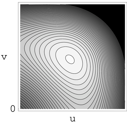
Figure 24: A contour plot of $\varepsilon_{GS}(u,v)$ in the absence of splitting, $\delta=0$. The global minimum at $u=v\neq 0$, saddle-points at $u=0,v\not=0$ and $u\not=0$, $v=0$, and a maximum at $u=v=0$ can clearly be seen.

Because there is only one local minimum, this fixed chemical potential result automatically applies to the minimization of $\varepsilon_{GS}$ at fixed total atom density $n$, with $\mu$ eliminated through Eq. (320). Thus we conclude that at $T=0$, the ground state of a Fermi gas interacting with an isotropic Feshbach resonance is a $p_{x}+ip_{y}$-wave superfluid throughout the BEC-BCS crossover.

In the BCS regime, this results agrees with the well-known prediction by Anderson and Morel Anderson and Morel (1961), who showed (in the context of A₁-phase of ³He) that a polarized $p$-wave BCS superconductor at $T=0$ is always in the $p_{x}+ip_{y}$ state. Thus, our above conclusion extends their result to the BEC ($\mu<0$) and crossover ($0<\mu<\epsilon_{F}$) regimes of a resonantly-paired superfluid.

We now compute this $p_{x}+ip_{y}$ ground state explicitly. To this end, we substitute $u=v$ into the ground state energy, Eq. (302) to obtain $\varepsilon_{GS}^{p_{x}+ip_{y}}[u]\equiv\varepsilon_{GS}[u,u]$

$$\frac{\varepsilon_{GS}^{p_{x}+ip_{y}}}{1+c_{2}}=2u^{2}\left[\omega_{0}-2\mu+a_{1}\ln(2a_{0}u)\right]+a_{1}u^{2}+4a_{2}u^{4},$$ (321)

and minimize it with the constraint Eq. (320). At fixed $\mu$, the saddle-point equation $\partial\varepsilon_{GS}^{p_{x}+ip_{y}}[u]/\partial u=0$ is given by

$$u[\omega_{0}-2\mu+a_{1}+a_{1}\ln(2a_{0}u)]+4a_{2}u^{2}=0.$$ (322)

As in the $s$-wave case, once the atom number constraint is implemented, the detailed behavior is quite different in three regimes, depending on the range of detuning $\omega_{0}$.

BCS regime:

For $\omega_{0}>2\epsilon_{F}$, closed-channel molecules (${\bf b}$) and the corresponding condensate are energetically costly leading to a small $u$. This justifies us to neglect the molecular contribution (first term) inside the number equation (320). Then, with approximation of $n_{0f}(\mu)$ by the normal state atom density (i.e., also ignoring the small condensate density there) (317) immediately gives $\mu\approx\epsilon_{F}$. Furthermore, similarly neglecting the subdominant quartic term, $a_{2}u^{4}$ inside $\varepsilon_{GS}^{p_{x}+ip_{y}}(\delta=0)$, Eq. (321), the corresponding saddle-point equation can then be solved analytically, giving

$$u^{\delta=0}_{p_{x}+ip_{y}} = \frac{1}{2a_{0}e}~{}e^{-(\omega_{0}-2\epsilon_{F})/a_{1}},$$

$$= e^{-11/6}\sqrt{2n\over\gamma_{p}}~{}e^{-(\omega_{0}-2\epsilon_{F})(1+\gamma_{p}\Lambda/k_{F})/(2\gamma_{p}\epsilon_{F})},$$

$$\hskip 56.9055pt\ \ \text{for}\ \ \omega_{0}>2\epsilon_{F},\ \delta=0,$$

that is indeed exponentially small in this BCS regime. The corresponding condensation energy density $\varepsilon_{GS}^{p_{x}+ip_{y}}(\delta)\equiv\varepsilon_{GS}^{p_{x}+ip_{y}}[u^{\delta}_{p_{x}+ip_{y}},\delta]$ is given by

$$\varepsilon_{GS}^{p_{x}+ip_{y}}(0) = -(1+c_{2})a_{1}(u^{0}_{p_{x}+ip_{y}})^{2},$$

$$= -4e^{-11/3}\ \epsilon_{F}n~{}e^{-(\omega_{0}-2\epsilon_{F})(1+\gamma_{p}\Lambda/k_{F})/(\gamma_{p}\epsilon_{F})}$$

$$\hskip 56.9055pt\ \ \text{for}\ \ \omega_{0}>2\epsilon_{F},\ \delta=0,$$

Within the same set of approximations it is also straightforward to compute the corresponding quantities for the $p_{x}$-state, obtaining ($u^{0}\equiv u^{\delta=0}$)

$$u^{0}_{p_{x}} = \frac{1}{a_{0}e^{3/2}}~{}e^{-(\omega_{0}-2\epsilon_{F})/a_{1}},$$

$$= e^{-14/6}\sqrt{8n\over\gamma_{p}}~{}e^{-(\omega_{0}-2\epsilon_{F})(1+\gamma_{p}\Lambda/k_{F})/(2\gamma_{p}\epsilon_{F})},$$

$$\varepsilon_{GS}^{p_{x}}(0) = -8e^{-14/3}\ \epsilon_{F}n~{}e^{-(\omega_{0}-2\epsilon_{F})(1+\gamma_{p}\Lambda/k_{F})/(\gamma_{p}\epsilon_{F})},$$ (326)

$$\hskip 56.9055pt\ \ \text{for}\ \ \omega_{0}>2\epsilon_{F},\ \delta=0,$$

that gives a ratio ${\cal R}(\delta=0)=\varepsilon_{GS}^{p_{x}+ip_{y}}(0)/\varepsilon_{GS}^{p_{x}}(0)=e/2$ of condensation energies for the two states, consistent with the numerical value reported in Ref. Anderson and Morel (1961) and thereby confirms that $p_{x}+ip_{y}$ state is energetically more favorable.

Crossover and BEC regimes:

For $\omega_{0}<2\epsilon_{F}$, it becomes favorable (even in $g_{p}\rightarrow 0$ limit) to convert a finite fraction of the Fermi sea (between $\omega_{0}$ and $2\epsilon_{F}$) into a BEC of closed-channel molecules. Consistent with this, the $\log$ contribution in Eq. (321) is no longer large, with $\varepsilon_{GS}^{p_{x}+ip_{y}}$ immediately giving a chemical potential that tracks the detuning according to $\mu\approx\omega_{0}/2$ with accuracy of $O(\gamma_{p})$.

As previously noted Andreev et al. (2004); Sheehy and Radzihovsky (2006b), we observe that the roles of number and gap equations interchange in the $\omega_{0}<2\epsilon_{F}$ regime, with the former determining the molecular condensate density and the latter giving the chemical potential. Consistent with this, the number equation, Eq. (320) then gives the growth of the bosonic condensate according to

$$u^{2}+v^{2}\approx\frac{n}{2(1+c_{2})}\left[1-\left({\omega_{0}\over 2\epsilon_{F}}\right)^{3/2}\theta(\omega_{0})\right],$$ (327)

reaching a maximum value of

$$u^{2}+v^{2}=\frac{n}{2(1+c_{2})},$$ (328)

for a negative detuning. As already noted above, it is remarkable that even for a large negative detuning the boson density never reaches its (ideal, $\gamma_{p}\ll 1$) maximum value of $n/2$ corresponding to the total atom density $n$. Instead, due to $p$-wave interaction that is strong at short scales, $c_{2}>0$, and a $p$-wave molecular condensate is depleted into open-channel atoms. We will nevertheless continue to refer to this range of detuning as the BEC regime.

Since as shown above, in the crossover and BEC regimes the ground state remains a $p_{x}+ip_{y}$-wave superfluid the $p$-wave order parameter is given by

$$u^{0}_{p_{x}+ip_{y}}\approx\frac{n^{1/2}}{2(1+c_{2})^{1/2}}\bigg{[}1 - \left({\omega_{0}\over 2\epsilon_{F}}\right)^{3/2}\theta(\omega_{0})\bigg{]}^{1/2},$$ (329)

$$\ \ \text{for}\ \ \omega_{0}<2\epsilon_{F}.$$

Anisotropic $p$-wave Feshbach resonance

We now analyze the more experimentally relevant anisotropic case Ticknor et al. (2004), where the triplet Feshbach resonance is split by dipolar interactions into a $m=\pm 1$ degenerate doublet resonance and an $m=0$ resonance, with $\omega_{\alpha}$ given by Eq. (VII.2.3). With the magnetic field ${\bf H}$ picking out a special direction (that we take to be $\hat{\bf x}$), the ground-state energy function $\varepsilon_{GS}$ is no longer rotationally invariant. Within our saddle-point approximation this uniaxial anisotropy only enters through the detuning part

$$\varepsilon_{GS}^{\text{anisot.}}[{\bf u},{\bf v}]=\omega_{0}(u^{2}+v^{2})+\delta(u_{y}^{2}+u_{z}^{2}+v_{y}^{2}+v_{z}^{2}).$$ (330)

With $\delta>0$, this uniaxial single-particle energy is clearly minimized by $u_{y}=u_{z}=v_{y}=v_{z}=0$, i.e., when ${\bf u}$ and ${\bf v}$ are parallel and point along ${\bf H}=H\hat{\bf x}$, corresponding to the $p_{x}$-wave ground state. In our more convenient ${\bf u}\cdot{\bf v}=0$ gauge choice, this $p_{x}$ state is equivalent to either ${\bf u}$ or ${\bf v}$ pointing along ${\bf H}$ and with the other vanishing. Furthermore, in this transverse gauge for a $p_{x}+ip_{y}$ state pwa (that, as we saw above is preferred by the interactions) in which neither ${\bf u}$ nor ${\bf v}$ vanish, $\varepsilon_{GS}^{\text{anisot.}}$ is clearly minimized by choosing the longer of the ${\bf u}$ and ${\bf v}$ to be along ${\bf H}=H\hat{\bf x}$, while the shorter one spontaneously selects a direction anywhere in the (yz-) plane perpendicular to ${\bf H}$. For $u=v$, their overall orientation is chosen spontaneously.

An explicit minimization over the direction of ${\bf u}$-${\bf v}$ orthogonal set confirms these arguments, giving

$$\varepsilon_{GS}^{\text{anisot.}}[u,v]=\omega_{0}(u^{2}+v^{2})+\delta~{}\text{Min}[u^{2},v^{2}].$$ (331)

It is convenient to take advantage of the exchange symmetry ${\bf u}\leftrightarrow{\bf v}$, $\varepsilon_{GS}[u,v]=\varepsilon_{GS}[v,u]$, and for $u\neq v$ (without loss of generality) always choose ${\bf u}$ to be the longer vector, with the other state physically equivalent. With this choice and Eq. (331) the ground-state energy is minimized by ${\bf u}$ directed along ${\bf H}$. The resulting ground state energy as a function of magnitudes $u$ and $v$, with $u>v$ and ${\bf u}=u\hat{\bf x}$ takes the form

$$\hat{\varepsilon}_{GS}[{\hat{u}},{\hat{v}}] = \hat{\omega}({\hat{u}}^{2}+{\hat{v}}^{2})+({\hat{u}}^{2}+{\hat{v}}^{2})^{2}+\frac{1}{2}({\hat{u}}^{2}-{\hat{v}}^{2})^{2}+\hat{\delta}{\hat{v}}^{2}+\hat{a}_{1}\left[({\hat{u}}^{2}+{\hat{v}}^{2})\ln({\hat{u}}+{\hat{v}})+{{\hat{u}}^{3}+{\hat{v}}^{3}\over{\hat{u}}+{\hat{v}}}\right],$$

$$\hskip 142.26378pt\qquad\qquad\qquad\qquad\qquad\text{for}\ \ u>v,\ {\bf u}=u\hat{\bf x},{\bf u}\perp{\bf v}.$$

where to simplify notation we introduced dimensionless variables

$$\hat{\omega} \equiv \big{(}\omega_{0}-2\mu+a_{1}\ln(a_{0}\sqrt{n})\big{)}/(a_{2}n),$$ (333)

$$\hat{\delta} \equiv \frac{\delta}{a_{2}n},$$ (334)

$$\hat{a}_{1} \equiv \frac{a_{1}}{a_{2}n},$$ (335)

$$\hat{\varepsilon}_{GS} \equiv {\varepsilon_{GS}\over(1+c_{2})a_{2}n^{2}}\equiv{\varepsilon_{GS}\over\varepsilon_{0}},$$ (336)

$${\hat{u}} \equiv \frac{u}{\sqrt{n}},\ \ {\hat{v}}\equiv\frac{v}{\sqrt{n}}.$$ (337)

As in the isotropic case above, the ground state as a function of detuning $\omega_{0}$ and dipolar splitting $\delta$ is found by minimizing $\hat{\varepsilon}_{GS}[{\bf u},{\bf v}]$ over magnitudes ${\bf u}$ and ${\bf v}$ with the constraint of the total atom density equation, Eq. (320)

$${\hat{u}}^{2}+{\hat{v}}^{2}=\frac{1}{2(1+c_{2})}\left(1-\left(\frac{\mu}{\epsilon_{F}}\right)^{3\over 2}\theta(\mu)\right).$$ (338)

Standard analysis shows that $\hat{\varepsilon}_{GS}[{\hat{u}},{\hat{v}}]$ generically has three physically distinctpwa (confined to ${\hat{u}}>{\hat{v}}>0$ quadrant) extrema: (i) ${\hat{u}}={\hat{v}}=0$ (normal state), (ii) ${\hat{u}}>0$, ${\hat{v}}=0$ ($p_{x}$-superfluid state), and (iii) ${\hat{u}}>{\hat{v}}>0$ ($p_{x}+ip_{y}$-superfluid state pwa ). At zero temperature for a fixed atom density the normal state is always a maximum with energy $\varepsilon_{GS}[0,0]\equiv\varepsilon_{GS}^{N}=0$. However, in contrast to the isotropic case, here the relative stability of the $p_{x}$ and $p_{x}+ip_{y}$ states crucially depends on the detuning $\omega_{0}$ and dipolar splitting $\delta$. This is summarized by the contour plots of $\varepsilon_{GS}(u,v)$ for $\delta=0$ (Fig. 24), $\delta$ small (Fig. 25) and $\delta$ large (Fig. 26). We now study these in detail.

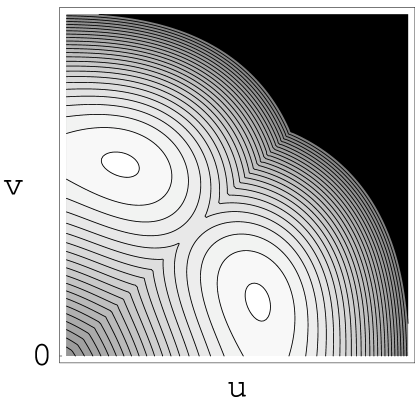
Figure 25: A contour plot of $\varepsilon_{GS}(u,v)$ in the presence of a small splitting $\delta$. The global minimum at $u\not=v\neq 0$ and saddle-points at $u=0,v\not=0$ and $u\not=0$, $v=0$, can clearly be seen.

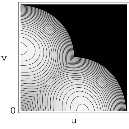
Figure 26: A contour plot of $\varepsilon_{GS}(u,v)$ in the presence of a large splitting $\delta$. Only the global minima at $u=0,v\not=0$ and $u\not=0$, $v=0$ are present

BCS regime:

As a generic property of the BCS regime, for $\omega_{0}>2\epsilon_{F}$, the molecules are energetically suppressed, and only exponentially small condensate is expected. The number equation then leads to $\mu\approx\epsilon_{F}$. It also allows us to neglect the subdominant quartic in ${\hat{u}}$ and ${\hat{v}}$ contributions inside $\varepsilon_{GS}$, Eq. (VII.2.3), allowing the corresponding saddle-point equation to be solved analytically. For the two candidate $p$-wave superfluid states we find:

$$u_{p_{x}+ip_{y}} = (1+\delta/a_{1})~{}e^{-\delta/2a_{1}}u^{0}_{p_{x}+ip_{y}},$$

$$= \frac{1}{2a_{0}e}(1+\delta/a_{1})~{}e^{-(\omega_{0}-2\epsilon_{F}+\delta/2)/a_{1}},$$

$$v_{p_{x}+ip_{y}} = (1-\delta/a_{1})~{}e^{-\delta/2a_{1}}v^{0}_{p_{x}+ip_{y}},$$

$$= \frac{1}{2a_{0}e}(1-\delta/a_{1})~{}e^{-(\omega_{0}-2\epsilon_{F}+\delta/2)/a_{1}},$$

$$\varepsilon_{GS}^{p_{x}+ip_{y}}(\delta) = -(1+\delta^{2}/a_{1}^{2})e^{-\delta/a_{1}}\varepsilon_{GS}^{p_{x}+ip_{y}}(0),$$

$$\hskip 85.35826pt\text{for}\ \ \omega_{0}>2\epsilon_{F},$$

and

$$u_{p_{x}} = u^{0}_{p_{x}},$$

$$= \frac{1}{a_{0}e^{3/2}}~{}e^{-(\omega_{0}-2\epsilon_{F})/a_{1}},$$

$$v_{p_{x}} = 0,$$

$$\varepsilon_{GS}^{p_{x}}(\delta) = \varepsilon_{GS}^{p_{x}}(0),$$

$$\ \ \text{for}\ \ \omega_{0}>2\epsilon_{F},$$

where the corresponding ground-state energies at finite splitting $\delta$ have been expressed in terms of $\delta=0$ energies, Eqs.(VII.2.3),(VII.2.3). The ratio of $p_{x}+ip_{y}$ and $p_{x}$ ground-state energies is then given by

$${\cal R}(\delta) = {\varepsilon_{GS}^{p_{x}+ip_{y}}\over\varepsilon_{GS}^{p_{x}}},$$ (341)

$$= {e\over 2}\left(1+{\delta^{2}\over a_{1}^{2}}\right)e^{-\delta/a_{1}},$$

and reduces to the previously found result of $e/2$ for $\delta=0$.

Consistent with the analysis of the “isotropic resonance” subsection, for low dipolar splitting $\delta$, ${\cal R}(\delta)>1$ and in the BCS regime the $p_{x}+ip_{y}$ superfluid pwa is the ground state, as seen on Fig. 25. However, ${\cal R}(\delta)$ reaches $1$ at $\delta_{c}^{BCS}$, given by

$$\delta_{c}^{BCS} = a_{1},$$

$$= {2\gamma_{p}\over 1+c_{2}}~{}\epsilon_{F},$$

signaling a quantum phase transition from the $p_{x}+ip_{y}$ to $p_{x}$ ground state for $\delta>\delta_{c}$ pwa . This is consistent with intrinsically positive quantity $v_{p_{x}+ip_{y}}(\delta)$, in Eq. (VII.2.3) turning negative (unphysical) for $\delta>\delta_{c}^{BCS}$.

BEC regime:

We can similarly evaluate the order parameters, ground state energies and the $p_{x}$-$p_{x}+ip_{y}$ quantum phase transition boundary in the opposite, BEC regime of a large negative detuning $\omega_{0}$ and $\mu<0$, which reduces the number equation, Eq. (338) to

$${\hat{u}}^{2}+{\hat{v}}^{2}=\frac{1}{2(1+c_{2})}\equiv\hat{n}_{B}.$$ (344)

As discussed for the isotropic resonance case, in the BEC regime the condensate is no longer exponentially small (given by a finite fraction of total atom density, as seen above), and as a result we can neglect the $\hat{a}_{1}$ terms in Eq. (VII.2.3) for small $\hat{a}_{1}$. Standard minimization of the resulting ground-state energy function, together with the number equation (344) gives for two extrema, one corresponding to a $p_{x}+ip_{y}$ superfluid pwa

$$u_{p_{x}+ip_{y}} = \frac{1}{\sqrt{2}}~{}n^{1/2}\left(\hat{n}_{B}+\hat{\delta}/2\right)^{1/2},$$

$$= \frac{1}{2}~{}n^{1/2}\left(\frac{1}{1+c_{2}}+\frac{5(1+c_{2})}{8c_{2}\gamma_{p}}\frac{\delta}{\epsilon_{F}}\right)^{1/2},$$

$$v_{p_{x}+ip_{y}} = \frac{1}{\sqrt{2}}~{}n^{1/2}\left(\hat{n}_{B}-\hat{\delta}/2\right)^{1/2},$$

$$= \frac{1}{2}~{}n^{1/2}\left(\frac{1}{1+c_{2}}-\frac{5(1+c_{2})}{8c_{2}\gamma_{p}}\frac{\delta}{\epsilon_{F}}\right)^{1/2},$$

$$\varepsilon_{GS}^{p_{x}+ip_{y}}(\delta) = -\varepsilon_{0}(\hat{n}_{B}^{2}+\hat{\delta}^{2}/8),$$

$$= -\left({2c_{2}\gamma_{p}\over 5(1+c_{2})^{2}}+{5(1+c_{2})^{2}\over 8c_{2}\gamma_{p}}\frac{\delta^{2}}{\epsilon_{F}^{2}}\right)\epsilon_{F}n,$$

and one corresponding to a $p_{x}$ superfluid

$$u_{p_{x}} = n^{1/2}\hat{n}_{B}^{1/2},$$

$$= \frac{1}{\sqrt{2(1+c_{2})}}~{}n^{1/2},$$

$$v_{p_{x}} = 0,$$

$$\varepsilon_{GS}^{p_{x}}(\delta) = -\frac{3}{2}\varepsilon_{0}~{}\hat{n}_{B}^{2},$$

$$= -\frac{3}{5}{c_{2}\gamma_{p}\over(1+c_{2})^{2}}~{}\epsilon_{F}n.$$

As argued earlier for the isotropic case, for low dipolar splitting $\delta$ the ground state is a $p_{x}+ip_{y}$ superfluid, with order parameter and ground-state energy given in Eq. (VII.2.3), illustrated on Fig. 25. As we can see from the form of $v_{p_{x}+ip_{y}}$ this minimum and the corresponding state disappears for $\hat{\delta}>2\hat{n}_{B}\equiv\hat{\delta}_{c}^{BEC}$, which gives the critical splitting

$$\delta^{BEC}_{c} = 2a_{2}n\hat{n}_{B},$$

$$= \frac{8}{5}{c_{2}\gamma_{p}\over(1+c_{2})^{2}}~{}\epsilon_{F}$$

for the quantum phase transition from $p_{x}+ip_{y}$ to $p_{x}$ superfluid pwa .

The behavior of the $p$-wave superfluid order parameters and ground state energy as a function of splitting $\delta$ and for full range of detuning $\omega_{0}$ is best mapped out numerically and gives a smooth interpolation between above extreme (BCS and BEC) limits derived above. However, the phase boundary $\delta_{c}(\omega_{0})$ for the quantum phase transition between $p_{x}+ip_{y}$ and $p_{x}$ superfluids can in fact be obtained analytically.

To this end we start at a large dipolar splitting, for which the $p_{x}$-superfluid ($u>v=0$) is a stable ground state and therefore the eigenvalues of the curvature matrix of $\varepsilon_{GS}[u,v]$ are positive in this state. We then locate the critical phase boundary $\delta_{c}(\omega_{0})$ by a point where the eigenvalue along $v$ direction changes sign, becoming negative and therefore signaling an instability toward development of a finite value of $v$ characteristic of the $p_{x}+ip_{y}$-superfluid.

To carry this out, we first minimize $\varepsilon_{GS}[u,v]$ to implicitly determine the value of $u_{p_{x}}$ (with $v_{p_{x}}=0$), that is given by:

$$(2\hat{\omega}+3\hat{a}_{1})+6{\hat{u}}_{p_{x}}^{2}+2\hat{a}_{1}\ln{\hat{u}}_{p_{x}}=0.$$ (348)

Although above saddle-point equation cannot be explicitly solved for $u_{p_{x}}$, it can be used to evaluate the eigenvalues of the curvature matrix at the $p_{x}$ minimum, and thereby determine the transition boundary $\delta_{c}(\omega_{0})$. Computing the eigenvalues of the curvature matrix of the ground-state energy at the $p_{x}$ minimum we find that $p_{x}$ superfluid is stable for

$$\hat{\delta}-\hat{a}_{1}-2{\hat{u}}_{p_{x}}^{2}>0,$$ (349)

which when combined with the atom number equation (338) gives (to lowest order in $\gamma_{p}$)

$$\hat{\delta}(\omega_{0}) \approx \hat{a}_{1}(\mu)+2\hat{n}_{B}\left(1-\left({\mu\over\epsilon_{F}}\right)^{3/2}\theta(\mu)\right),$$ (350)

$$\approx \cases{\hat{\delta}_{c}^{BCS}=\frac{5}{4c_{2}}\ ,&\text{for $\omega_{0}>2\epsilon_{F}$}\cr\hat{\delta}_{c}^{cross.+BEC}(\omega_{0})=\left(\frac{5}{4c_{2}}-\frac{1}{1+c_{2}}\right)\left({\omega_{0}\over 2\epsilon_{F}}\right)^{3/2}\theta(\omega_{0})+\frac{1}{1+c_{2}}\ ,&\text{for $\omega_{0}<2\epsilon_{F}$},\cr}$$ (351)

for the (dimensionless) critical boundary illustrated in Fig. 27, with the system transitioning into the $p_{x}+ip_{y}$-superfluid pwa for $\delta<\delta_{c}(\omega_{0})$. In above we used small $\gamma_{p}$ (narrow Feshbach resonance) approximation for the chemical potential $\mu(\omega_{0})$ (derived above) appropriate for different regimes. As anticipated the phase boundary $\delta_{c}(\omega_{0})$ smoothly interpolates as a function of detuning between the BCS and BEC results found in Eqs.(VII.2.3), (VII.2.3). Since for all values of the dimensionless coupling $c_{2}=\gamma_{p}\Lambda/k_{F}$, $\hat{\delta}_{c}^{BEC}<\hat{\delta}_{c}^{BCS}$, for $\hat{\delta}$ falling between these two values we predict a continuous quantum phase transition at a critical value of detuning, given by (to ${\cal{O}}(\gamma_{p})$)

$$\omega_{0}^{c}(\delta)\approx 2\epsilon_{F}\left({\delta-\delta_{c}^{BEC}\over\delta_{c}^{BCS}-\delta_{c}^{BEC}}\right)^{2/3}.$$ (352)

Figure 27: The phase diagram of an anisotropic $p$-wave superfluid at zero temperature, illustrating a phase boundary of (dimensionless) dipolar splitting $\hat{\delta}_{c}(\omega_{0})$ as function of detuning, that marks a phase boundary of a continuous quantum phase transition between a $p_{x}$- and $p_{x}+ip_{y}$-superfluid.

VII.3 Finite temperature: phases and transitions in a $p$-wave resonant Fermi gas

We now extend our study of the phase behavior of a $p$-wave resonant gas to finite temperature. This involves a calculation of the free-energy density, $f_{p}[{\bf B}]$, Eq. (286), and its minimization along the lines similar to the above $T=0$ analysis of the ground-state energy density $\varepsilon_{GS}[{\bf B}]$. The former amounts to a computation of the polarization tensor $I^{(T)}_{\alpha\beta}[{\bf B}]$, Eq. (296), details of which we relegate to Appendix C.

The upshot of detailed calculations, presented in the Appendix C, is that (as usual) at finite $T$ the low-energy singularities arising from Fermi-surface low-energy contributions to $I_{\alpha\beta}[{\bf B}]$ are cutoff by $T$. Consequently, (in contrast to the $T=0$ case, above), the free energy, $f_{p}[{\bf B}]$ is an analytic function of ${\bf B}$, that at high temperatures, where $|{\bf B}|$ is small is Taylor-expandable in powers of the gauge-invariant tensor $\bar{B}_{\alpha}B_{\beta}$. Naturally, in the isotropic case $\omega_{\alpha}=\omega_{0}$ and $f_{p}[{\bf B}]$ only involves rotationally invariant traces of the powers of a tensor $Q_{\alpha\beta}=\bar{B}_{\alpha}B_{\beta}$ and its transpose $Q_{\beta\alpha}$.

Within the saddle-point approximation only the quadratic contribution is anisotropic, and the resulting free-energy density is given by a standard Landau form

$$f_{p}[{\bf B}]=\sum_{\alpha=x,y,z}t_{\alpha}|B_{\alpha}|^{2}+\lambda_{1}\left({\bf\bar{B}}\cdot{\bf B}\right)^{2}+\lambda_{2}|{\bf B}\cdot{\bf B}|^{2},$$

where, because of the dipolar-anisotropy splitting $t_{x}(T,\omega_{0})<t_{y}(T,\omega_{0})=t_{z}(T,\omega_{0})\equiv t_{\perp}(T,\omega_{0})$, reflecting uniaxial symmetry of the system, and these parameters vanish linearly at respective $T_{c}^{\prime}s$, with

$$t_{x}(T,\omega_{0}) \sim T-T_{c}^{x}(\omega_{0}),$$ (354)

$$t_{\perp}(T,\omega_{0}) \sim T-T_{c}^{\perp}(\omega_{0}),$$

and

$$T_{c}^{x}(\omega_{0})>T_{c}^{\perp}(\omega_{0}).$$ (355)

The parameters $\lambda_{1,2}$ are only weakly temperature dependent.

Beyond the saddle-point approximation, we expect that generically only the gauge-invariance is preserved by all the terms in $f_{p}[{\bf B}]$ and lack of rotational symmetry for finite $\delta$ will be reflected by all terms. However, for our purposes it will be sufficient to keep only the dominant non-rotational invariant contribution entering through the quadratic term as reflected in $f_{p}[{\bf B}]$ above. In terms of ${\bf u}$ and ${\bf v}$ parametrization the free-energy density is given by

$$f_{p}[{\bf u},{\bf v}]=\sum_{\alpha=x,y,z}t_{\alpha}(u_{\alpha}^{2}+v_{\alpha}^{2})+\lambda_{1}(|{\bf u}|^{2}+|{\bf v}|^{2})^{2}+\lambda_{2}\left((|{\bf u}|^{2}-|{\bf v}|^{2})^{2}+4({\bf u}\cdot{\bf v})^{2}\right),$$ (356)

where the ratio of $4$ between the two $\lambda_{2}$ terms is a generic feature that is a reflection of the underlying gauge-invariance.

VII.3.1 Isotropic

In the isotropic case ($\delta=0$), $t_{x}=t_{\perp}\equiv t(T)$, and the free-energy density is fully rotationally invariant, given by

$$f_{p}^{iso}[{\bf B}]=t|{\bf B}|^{2}+\lambda_{1}\left({\bf\bar{B}}\cdot{\bf B}\right)^{2}+\lambda_{2}|{\bf B}\cdot{\bf B}|^{2}.$$ (357)

For $t>0$ ($T>T_{c}$), $f_{p}^{iso}[{\bf B}]$ is minimized by ${\bf B}=0$ and the gas is in its normal (nonsuperfluid) phase. Upon lowering $T$ below $T_{c}$, a minimum develops at a finite value of ${\bf B}$. As can be seen from the its expression in terms of ${\bf u}$ and ${\bf v}$, Eq. (359) the minimum is at $u=v$ and ${\bf u}\cdot{\bf v}=0$ (or any of its gauge-equivalent states corresponding to unequal and nontransverse ${\bf u}$ and ${\bf v}$). Thus, the finite-$T$ normal-to-superfluid transition is to a $p_{x}+ip_{y}$-superfluid (SF${}_{p_{x}+ip_{y}}$), consistent with our earlier finding Anderson and Morel (1961) that the ground state is a $p_{x}+ip_{y}$-superfluid, for all detunings. At this transition the global $U(1)$ gauge-symmetry is spontaneously broken, corresponding to a choice of a phase of ${\bf B}$ or equivalently the relative orientation and magnitudes of ${\bf u}$ and ${\bf v}$ (as long as they are not parallel or one of them does not vanish, since this would correspond to a $p_{x}$ state that is not connected to the $p_{x}+ip_{y}$ state by a gauge transformation). In addition, an arbitrary choice of an overall orientation of ${\bf B}$ (i.e., of the ${\bf u}-{\bf v}$ frame, that by gauge-choice can be taken to be orthogonal) spontaneously breaks $O(3)$ rotational symmetry. Clearly time-reversal symmetry is also spontaneously broken in the $p_{x}+ip_{y}$-superfluid state.

This finite-temperature transition is in the complex $O(3)$ universality class, which can be thought of as a well-explored real $O(6)$ modelZinn-Jistin (2002), explicitly broken by $\lambda_{2}$ crystal symmetry-like breaking fields, analogous to $O(3)$ ferromagnet in a crystal-fields due to spin-orbit coupling to a lattice. Its critical behavior has been extensively explored by Vicari, et al. Calabrese et al. (2004).

VII.3.2 Anisotropic

We now turn to the more experimentally relevant uniaxially anisotropic case, of a Feshbach-resonance triplet split by $\delta>0$ (as described above) by dipolar interactions in the presence of an external magnetic field ${\bf H}=H\hat{\bf x}$. The dipolar splitting considerably enriches the phase diagram, allowing for three possible phase diagram topologies, illustrated in Figs 9, 10 and 11. In terms of the complex $O(3)$ model dipolar-splitting leads to an easy-axis (Ising) anisotropy, with the free-energy density given by

$$f^{anisot}_{p}\left[{\bf B}\right] = t_{x}|B_{x}|^{2}+t_{\perp}|{\bf B}_{\perp}|^{2}+\lambda_{1}\left({\bf\bar{B}}\cdot{\bf B}\right)^{2}+\lambda_{2}|{\bf B}\cdot{\bf B}|^{2},$$ (358)

$$= t_{x}(u_{x}^{2}+v_{x}^{2})+t_{\perp}(u_{\perp}^{2}+v_{\perp}^{2})+\lambda_{1}(|{\bf u}|^{2}+|{\bf v}|^{2})^{2}+\lambda_{2}\left((|{\bf u}|^{2}-|{\bf v}|^{2})^{2}+4({\bf u}\cdot{\bf v})^{2}\right),$$ (359)

where $\perp$ indicates two components in the plane perpendicular to the external magnetic field ${\bf H}$ axis that we have taken to be $\hat{\bf x}$. For $t_{x}<t_{\perp}$ it is clear that $B_{x}$ part of ${\bf B}$ will order first, with ${\bf B}_{\perp}=0$. Namely, since $T_{c}^{x}>T_{c}^{\perp}$, ${\bf u}$ and ${\bf v}$ will always both order parallel to the $x$-axis, showing that for arbitrary small splitting $\delta>0$ and arbitrary detuning $\omega_{0}$, the finite temperature normal to $p$-wave superfluid transition is always to the $p_{x}$-superfluid SF${}_{p_{x}}$. We designate this upper-critical temperature by $T_{c2}(\omega_{0})$ and expect it to be set (up to renormalization by fluctuations) by $T_{c}^{x}(\omega_{0})$. Clearly from the structure of $f^{anisot}_{p}[{\bf B}]$, Eq. (358), the noncritical (“massive”) ${\bf B}_{\perp}$ component can be safely integrated out at the N-SF${}_{p_{x}}$ transition, leaving a Landau model of a single complex order parameter $B_{x}$. Hence the finite-$T$ N-SF${}_{p_{x}}$ classical transition is in 3D XY universality class, at which only a global $U(1)$ gauge symmetry is broken.

What follows upon further lower the temperature qualitatively depends on the strength of the dipolar splitting $\delta$. This follows from the zero-temperature analysis of Sec. VII.2.3 and is summarized by phase diagrams in Figs 9, 10 and 11.

For weak (normalized) Feshbach resonance dipolar splitting $0<\hat{\delta}<\hat{\delta}_{c}^{BCS}$, upon further lowering temperature from a $p_{x}$-superfluid phase, the system always undergoes a transition to a $p_{x}+ip_{y}$-superfluid for all detuning $\omega_{0}$; we designate this critical temperature by $T_{c1}(\omega_{0})$. To see this, we observe that for this low range of $\delta$, the parameter $t_{\perp}$ becomes negatives with reduced $T$ and thereby leads to another critical temperature at which the ${\bf B}_{\perp}$ component also orders. This ordering takes place in the presence of a finite $p_{x}$ order parameter $B_{x0}$, within mean-field theory given by

$$B_{x0}=\sqrt{-t_{x}\over 2(\lambda_{1}+\lambda_{2})}.$$ (360)

The resulting Landau theory for ${\bf B}_{\perp}$ is then given by

$$f_{p_{x}\rightarrow p_{x}+ip_{y}} = (t_{\perp}+2\lambda_{1}|B_{x0}|^{2})|{\bf B}_{\perp}|^{2}+(\lambda_{1}+\lambda_{2})|{\bf B}_{\perp}|^{4}+\lambda_{2}\left(\bar{B}_{x0}^{2}{\bf B}_{\perp}\cdot{\bf B}_{\perp}+B_{x0}^{2}{\bf\bar{B}}_{\perp}\cdot{\bf\bar{B}}_{\perp}\right),$$ (361)

$$= \left(\tilde{t}_{\perp}+2\tilde{\lambda}\cos(2\varphi_{\perp}-2\varphi_{x,0})\right)|{\bf B}_{\perp}|^{2}+\lambda|{\bf B}_{\perp}|^{4}$$ (362)

where $\lambda\equiv\lambda_{1}+\lambda_{2}$ and

$$\tilde{\lambda} \equiv \lambda_{2}|B_{x0}|^{2}={\lambda_{2}\over 2(\lambda_{1}+\lambda_{2})}|t_{x}|,$$ (363)

$$\tilde{t}_{\perp} \equiv t_{\perp}+2\lambda_{1}|B_{x0}|^{2}=t_{\perp}+{\lambda_{1}\over\lambda_{1}+\lambda_{2}}|t_{x}|.$$ (364)

We note that at this transition the phase $\varphi_{\perp}$ of ${\bf B}_{\perp}$ locks to the phase $\varphi_{x,0}$ of $B_{x,0}$ so that the relative phase is $\pm\pi/2$. This is exactly what is expected upon ordering into one of the two degenerate $p_{x}\pm ip_{y}$ states. We thus find that the SF${}_{p_{x}}$ to SF${}_{p_{x}+ip_{y}}$ transition is modified by the presence of $p_{x}$ order and takes place at

$$t_{\perp}(T) = 2(\lambda_{2}-\lambda_{1})|B_{x0}|^{2},$$ (365)

$$= -t_{x}(T){\lambda_{2}-\lambda_{1}\over\lambda_{2}+\lambda_{1}},$$

which then in turn determines $T_{c1}(\omega_{0})$. Since the $U(1)$ gauge-symmetry is already broken in the $p_{x}$-superfluid phase and since, as seen above $\varphi_{\perp}$ is automatically locked to $\varphi_{x,0}$, the remaining symmetries that are broken at this transition are the $O(2)$ rotations of ${\bf B}_{\perp}$ about the $x$-axis (set by the magnetic field $H$) and the time-reversal symmetry associated with a choice of one of the locking angles $\pm\pi/2$, corresponding to angular momentum projection $m=\pm 1$. Thus the SF${}_{p_{x}}$ to SF${}_{p_{x}+ip_{y}}$ transition is also in the well-studied 3D XY universality class. Above results are summarized by a finite temperature part of the phase diagram, illustrated in Fig. 28

Figure 28: Finite-temperature phase diagram illustrating continuous transitions between normal (N), $p_{x}$-superfluid (SF${}_{p_{x}}$) and ${p_{x}+ip_{y}}$-superfluid (SF${}_{p_{x}+ip_{y}}$). The parameters $t_{x}(T)<t_{\perp}(T)$ are reduced temperatures split by $\delta$. Only $t_{x}<t_{\perp}$ part of the figure is physically relevant.

At intermediate dipolar splitting $\hat{\delta}_{c}^{BEC}<\hat{\delta}<\hat{\delta}_{c}^{BCS}$, the N-SF${}_{p_{x}}$ transition can also be followed by the SF${}_{p_{x}}$ to SF${}_{p_{x}+ip_{y}}$ transition, but only for detuning $\omega_{0}>\omega_{0c}(T)$, as illustrated in Fig .10. The zero-temperature critical frequency $\omega_{0c}$ (with limits $\omega_{0c}(\delta\rightarrow\delta_{c}^{BCS})\rightarrow+\infty$ and $\omega_{0c}(\delta\rightarrow\delta_{c}^{BEC})\rightarrow-\infty$) is given by Eq. (352) and $\omega_{0c}(T)$ is its finite-$T$ extension. Hence, for this intermediate range of $\delta$, we predict on general grounds that this SF${}_{p_{x}}$– SF${}_{p_{x}+ip_{y}}$ phase boundary $T_{c1}(\omega_{0})$ has a maximum. Thus at fixed $T$ the gas for this range of parameters should exhibit a reentrant $SF_{p_{x}}\rightarrow SF_{p_{x}+ip_{y}}\rightarrow SF_{p_{x}}$ transition with detuning $\omega_{0}$.

Finally, for large dipolar splitting $\hat{\delta}_{c}^{BCS}<\hat{\delta}$, $p_{x}$-superfluid is stable below $T_{c2}(\omega_{0})$ throughout, as illustrated in Fig.11. We note, however, that for a Feshbach resonance splitting much larger than the Fermi energy, we expect that on sufficiently short time scales (set by time scale for energy relaxation in the system) the two ($m=0$ and $m=\pm 1$) split Feshbach resonances will act independently, so that one can come in resonance with each of them separately. If so, either Fig. 11 or 9 will be experimentally observed, depending on to which of the two resonances, $m=0$ or $m=\pm 1$, respectively the system has been tuned.

All of the above discussed transitions are quite conventional and should be experimentally identifiable through (among other signatures) their standard universal thermodynamic singularities (e.g., in heat capacity). Furthermore, the phases should be distinguishable through their spectroscopic properties, with the normal state gapless throughout, and for positive chemical potential, the $p_{x}$-superfluid displaying a gap with an equatorial line of nodes, i.e., for ${\bf k}_{nodes}^{p_{x}}={\bf k}^{\perp}_{F}$, and $p_{x}+ip_{y}$-superfluid exhibiting a gap with nodes at the north and south pole, i.e., at ${\bf k}_{nodes}^{p_{x}+ip_{y}}=\pm k_{F}\hat{\bf z}$.

In addition to above transitions that are characterizable by an order parameter, we expect the $p$-wave superfluid to exhibit a number of non-Landau type of (the so-called) topological transitions at $\mu=0$. The simplest argument for the existence of such transitions is the fact that a $p$-wave superfluid exhibits the aforementioned gapless excitations around Fermi surface for $\mu>0$, and is gapped to single-particle excitations for $\mu<0$, as clearly seen in $E_{\bf k}$, Eq. (287). Thus we predict continuous $SF_{p_{x}}^{gapless}\rightarrow SF_{p_{x}}^{gapped}$ and $SF_{p_{x}+ip_{y}}^{gapless}\rightarrow SF_{p_{x}+ip_{y}}^{gapped}$ transitions at $\mu=0$. One might expect a clear signature of such transitions from the change in the low-$T$ thermodynamic behavior, e.g., with the heat capacity changing from a power-law in $T$ to an activated form, with gap for $\mu<0$ set by the molecular binding energy. However, a collective sound mode, present in any superfluid, that contributes power-law in $T$ contributions, might obscure the distinction between the $\mu>0$ and $\mu<0$ $p$-wave superfluid phases. Local spectroscopic experimental probes (some atomic gas analog of tunneling experiments) should prove useful for detection of these transitions. Despite a lack of local Landau order parameter, these weakly- and strongly-paired $p$-wave superfluids are distinguishable by their topological properties Volovik (1992, 2003, 2006); Klinkhamer and Volovik (2004); Read and Green (2000), as we discuss in the next section.

VIII Topological phase transitions and non-Abelian statistics

In addition to the rich (but conventional) phenomenology of $p$-wave resonant gases obtained in previous subsections, as we will show next, they can also exhibit a more subtle (in some cases topological) order and associated phase transitions, that cannot be classified by a local order parameter, nor associated Landau theory Chaikin and Lubensky (2000). The existence of such continuous non-Landau type phase transitions have long been appreciated in the literature. Examples range from Anderson’s metal-insulator transition and transitions between different quantum Hall ground states to the well-understood Kosterlitz-Thouless transition (e.g., in superfluid films) and two-dimensional melting, all separating two disordered states undistinguished by any local order parameter or conventional symmetry operation.

VIII.1 $P$-wave superfluid in $3$ dimensions

It is remarkable that $p_{x}$- and $p_{x}+ip_{y}$-superfluids are examples of a system, that can undergo such non-Landau type phase transition when the chemical potential changes sign. In three dimensions this can be simply seen from the qualitative change in the spectrum $E_{\bf k}$, Eq. (287) of single-particle fermionic excitations, that for the $p_{x}$ and $p_{x}+ip_{y}$ states

$$(B_{x},B_{y},B_{z})_{p_{x}} = \frac{\Delta}{2g_{p}}~{}(1,0,0),$$ (366)

$$(B_{x},B_{y},B_{z})_{p_{x}+ip_{y}} = \frac{\Delta}{2g_{p}}~{}(1,i,0),\$$ (367)

are respectively given by

$$E^{p_{x}}_{\bf k} = \sqrt{\left(\frac{k^{2}}{2m}-\mu\right)^{2}+|\Delta|^{2}k_{x}^{2}},$$ (368)

$$E^{p_{x}+ip_{y}}_{\bf k} = \sqrt{\left(\frac{k^{2}}{2m}-\mu\right)^{2}+|\Delta|^{2}(k_{x}^{2}+k_{y}^{2})},$$ (369)

with $\Delta$ the maximum gap of each state, related to the corresponding order parameter. Clearly, in a $p_{x}$-superfluid, for $\mu>0$, $E^{p_{x}}_{{\bf k}}=0$ (i.e., gapless) for $k_{x}=0$ and $k_{y}$, $k_{z}$ arbitrary, and for $\mu<0$, $E^{p_{x}}_{{\bf k}}>0$ (i.e., gapped) for all ${\bf k}$. Similarly, in a $p_{x}+ip_{y}$-superfluid, for $\mu>0$, $E^{p_{x}+ip_{y}}_{{\bf k}}=0$ (i.e., gapless) for $k_{z}=\sqrt{2m\mu}$ and $k_{x}=k_{y}=0$, and for $\mu<0$, $E^{p_{x}+ip_{y}}_{{\bf k}}>0$ (i.e., gapped) for all ${\bf k}$. Physically these spectral distinctions arise because for $\mu>0$, a phase that we refer to as $SF_{p}^{\text{w}eak}$, the pairing is a collective Fermi surface phenomenon and finite angular momentum forces the gap to vanish on some subspace of the Fermi surface. On the other hand, for $\mu<0$, in the $SF_{p}^{\text{s}trong}$ the gap is single-pair of fermions phenomenon and is simply set by the molecular binding energy, independent of the angular momentum state of the molecule.

These changes in the spectrum lead to qualitatively distinct single-particle correlation functions and therefore require a genuine quantum phase transition (illustrated in Figs. 9, 10, 11) separating two distinct (weakly- and strongly-paired) $p_{x}$- and two distinct (weakly- and strongly-paired) $p_{x}+ip_{y}$-superfluids, as $\mu$ changes from positive to negative, respectively.

In a classic BCS $p$-wave paired superfluid, such as He³, $\mu$ is always positive and these transitions are not experimentally accessible. However, in $p$-wave resonant atomic gases they should be easily realizable (if a $p$-wave superfluid is produced) by changing the detuning parameter $\omega_{0}$ (controlled by an external magnetic field), that is, as we have shown in Sec. VII, is closely tracked (up to terms of the order of $g_{p}$) by $\mu$.

In addition to the above quasiparticle spectrum and correlation function argument for the transition at $\mu=0$, the existence of the $SF_{p_{x}+ip_{y}}^{\text{w}eak}\rightarrow SF_{p_{x}+ip_{y}}^{\text{s}trong}$ transition can be also seen by noting that the two types of $p_{x}+ip_{y}$-superfluids can be distinguished by topological order as discussed in detail in Refs. Volovik (2003); Klinkhamer and Volovik (2004); Volovik (2006). Although, as argued above a spectral distinction between $\mu>0$ and $\mu<0$ $p_{x}$-superfluids exists, and therefore we expect a corresponding $SF_{p_{x}}^{\text{w}eak}\rightarrow SF_{p_{x}}^{\text{s}trong}$ transition at $\mu=0$, we are not aware of any topological distinction between these two phases similar to the $p_{x}+ip_{y}$ classification. For the rest of the section, below, we will focus on the analogous transition in two dimensions, where for a $p_{x}+ip_{y}$-superfluid clearly no spectral distinction exists, with both $SF_{p_{x}+ip_{y}}^{\text{w}eak}$ and $SF_{p_{x}+ip_{y}}^{\text{s}trong}$ gapped, but still distinguishable by topological order.

VIII.2 $P$-wave superfluid in $2$ dimensions

The three-dimensional calculations of this paper, arguing for the existence of a $p$-wave superfluid can be easily extended to two dimensions, with only minor quantitative distinctions (e.g., the dimensionless parameter $c_{2}$ in $2D$ scales logarithmically with the uv cutoff $\Lambda$). Thus, we expect the existence of a fully-gapped two-dimensional $p_{x}+ip_{y}$-superfluid for $\mu>0$ and $\mu<0$. As we will see, a plethora of especially interesting phenomena takes place in such a system, that we expect to be realizable by confining the degenerate atomic gas to a highly oblate magnetic trap.

Although much of our discussion of this system follows an excellent paper by N. Read and D. Green, Ref. Read and Green (2000), as well as Refs. Volovik (2003, 2006); Gurarie and Radzihovsky , we elaborate on details of the analysis (particularly on the existence of the zero modes), and thereby hope to elucidate a number of points discussed there. Furthermore, while above papers are well-known and appreciated in the quantum Hall community, they are less familiar to the atomic community and thus, their main results are worth elaborating on here.

Following Ref. Read and Green (2000), let us first construct a ground state wave function of a two-dimensional $p_{x}+ip_{y}$ superfluid. As discussed in Sec. V.2 its mean-field Hamiltonian (valid in the narrow-resonance limit) follows directly from Eq. (V.2.1), with the substitution $\hat{b}_{{\bf p},\alpha}\rightarrow\delta_{{\bf p},0}B_{\alpha}$ and Eq. (367), and is given by

$$\hat{H}-\mu~{}\hat{N}_{f} = \sum_{{\bf k}}\xi_{k}~{}\hat{a}^{\dagger}_{{\bf k}}\hat{a}_{{\bf k}}-\frac{1}{2}\sum_{{\bf k}}~{}\bigg{[}\Delta\left(k_{x}+ik_{y}\right)~{}\hat{a}^{\dagger}_{{\bf k}}\hat{a}^{\dagger}_{-{\bf k}}$$ (370)

$$+ \Delta\left(k_{x}-ik_{y}\right)~{}\hat{a}_{-{\bf k}}\hat{a}_{{\bf k}}\bigg{]}.$$ (371)

Here we fix the phase of $\Delta$ by choosing $\Delta=\bar{\Delta}$ and, as before, $\xi_{k}$ is given by Eq. (191),

$$\xi_{k}=\frac{k^{2}}{2m}-\mu.$$

This Hamiltonian is diagonalized by a unitary transformation to the Bogoliubov quasiparticles

$$\hat{\gamma}_{\bf k} = u_{\bf k}^{*}\hat{a}_{\bf k}+v_{\bf k}^{*}\hat{a}^{\dagger}_{-{\bf k}},$$ (372)

$$\hat{\gamma}^{\dagger}_{{\bf k}} = v_{\bf k}\hat{a}_{-{\bf k}}+u_{\bf k}\hat{a}^{\dagger}_{{\bf k}},$$ (373)

taking the form

$$\hat{H}=E_{GS}+\sum_{k}E_{\bf k}\hat{\gamma}^{\dagger}_{\bf k}\hat{\gamma}_{\bf k}.$$ (374)

The ground state of this Hamiltonian is similar to its $s$-wave counterpart Eq. (194), and is given by

$$\left|{\rm BCS}\right\rangle=\prod_{\bf k}\left(u^{*}_{\bf k}+v^{*}_{\bf k}~{}a^{\dagger}_{-{\bf k}}a^{\dagger}_{{\bf k}}\right)\left|0\right\rangle.$$ (375)

with each pair ${\bf k}$, $-{\bf k}$ in the product taken only once. Here $u_{\bf k}$, $v_{\bf k}$ are $p$-wave analogs of Eq. (191), and satisfy the Bogoliubov-de-Gennes equations

$$\left(\matrix{\xi_{k}&-\Delta\left(k_{x}+ik_{y}\right)\cr-\Delta\left(k_{x}-ik_{y}\right)&-\xi_{k}}\right)\left(\matrix{u_{\bf k}\cr v_{{\bf k}}}\right)=E_{k}\left(\matrix{u_{\bf k}\cr v_{{\bf k}}}\right),$$ (376)

The solution of these equations is straightforward with the result Eq. (369) and with normalized $u_{\bf k}$, $v_{\bf k}$ being

$$u_{\bf k} = -\sqrt{\frac{E_{\bf k}+\xi_{k}}{2E_{\bf k}}},$$ (377)

$$v_{\bf k} = \frac{\left(k_{x}-ik_{y}\right)\Delta}{\sqrt{2E_{\bf k}\left(E_{\bf k}+\xi_{k}\right)}}$$ (378)

We note that unlike the $s$-wave case Eq. (195), the relative phase of $u_{\bf k}$ and $v_{\bf k}$ is nonzero. Let us construct a real space version of Eq. (375). It is given by

$$\Psi({\bf r}_{1},{\bf r}_{2},\dots)=\sum_{P}(-1)^{P}g({\bf r}_{P_{1}}-{\bf r}_{P_{2}})~{}g({\bf r}_{P_{3}}-{\bf r}_{P_{4}})\dots.$$ (379)

Here ${\bf r}_{i}$ are two-dimensional vectors denoting the position of the $i$-th fermion, and $g({\bf r})$ is a Cooper-pair (or molecular) wavefunction given by

$$g({\bf r})=\int{d^{2}k\over(2\pi)^{2}}~{}e^{i{\bf k}\cdot{\bf r}}~{}\frac{v_{\bf k}}{u_{\bf k}}.$$ (380)

$P$ stands for a permutation of numbers $1,2,\dots,N_{f}$, where $N_{f}$ is the total number of fermions, and $(-1)^{P}$ is the sign of the permutation, thereby enforcing the antisymmetrization of the many-atom ground-state wavefunction. Notice that $g({\bf r})=-g(-{\bf r})$ due to the $p$-wave symmetry of the superfluid (since $u_{\bf k}=u_{-{\bf k}}$, $v_{{\bf k}}=-v_{-{\bf k}}$).

Now suppose $\mu>0$. Then at small $k\ll\sqrt{2m\mu}$ or equivalently $|{\bf r}|\gg n^{-1/3}$, we can estimate the function to be integrated in Eq. (380) to go as

$$\frac{v_{\bf k}}{u_{\bf k}}=\frac{k_{x}-ik_{y}}{E_{\bf k}+\xi_{k}}\Delta\sim\frac{k_{x}-ik_{y}}{k^{2}}.$$ (381)

It immediately follows that for $|{\bf r}|\gg l$,

$$g({\bf r})\sim\frac{1}{z},$$ (382)

where $z$ is the complex number representing the two-dimensional vector ${\bf r}=x\hat{\bf x}+y\hat{\bf y}$ as $z=x+iy$. Therefore, for $\mu>0$ the wave function takes the form

$$\Psi(z_{1},z_{2},\dots)=\sum_{P}(-1)^{P}\frac{1}{z_{P_{1}}-z_{P_{2}}}~{}\frac{1}{z_{P_{3}}-z_{P_{4}}}\dots.$$ (383)

This wave function occurs in the context of the quantum Hall effect (modulo the Gaussian and Jastrow factors not essential for the present discussion) and is called the Pfaffian or Moore-Read state Moore and Read (1991).

To understand the connection with the quantum Hall effect, we recall that for the last few years attempts have been made to realize quantum Hall states Wilkin and Gunn (2000); Cooper et al. (2001) out of Bose-Einstein condensates by rotating them Schweikhard et al. (2004). In the $p_{x}+ip_{y}$ condensate, thanks to the relative angular momentum $\ell=1$ of each Cooper pair (or closed-channel molecule), the (fermionic) condensate already automatically rotates and therefore does not require any externally imposed rotation to be in the quantum Hall ground state.

A key observation is that for $\mu<0$ $u_{\bf k}/v_{\bf k}\sim k_{x}-ik_{y}$ at small $k$ and $g({\bf r})$ no longer has the power-law fall off characteristic of the quantum Hall-like ground state in Eq. (383). Instead, the integral in Eq. (380) is then dominated by large $k$, and generally we expect that $g({\bf r})$ will be an exponentially decaying function. The authors of Ref. Read and Green (2000) referred to the $\mu<0$ as the strongly-coupled phase. For BCS-BEC condensates studied here, $\mu<0$ corresponds to the BEC regime obtained for negative detuning $\omega_{0}$.

As mentioned above, despite the qualitative distinction in the ground-state wavefunctions, in a two dimensions $E_{k}>0$, i.e., gapped for all ${\bf k}$, for both $\mu>0$ and $\mu<0$. The only special point where there are gapless excitations is $\mu=0$. Nevertheless given the qualitative distinction between the ground states at $\mu>0$ and $\mu<0$, they much be separated by a quantum phase transition at the gapless point $\mu=0$. The situation is again reminiscent of quantum Hall transitions where gapless points separates gapped quantum Hall states.

Although this transition at $\mu=0$ is not of Landau type (not exhibiting any obvious local order parameter) the weakly- ($\mu>0$) and strongly-paired ($\mu<0$) $p_{x}+ip_{y}$ states are topologically distinct and therefore the transition is topological. The topological distinction lies in the properties of the two complex functions $u_{\bf k}$ and $v_{\bf k}$, constrained by $|u_{\bf k}|^{2}+|v_{\bf k}|^{2}=1$. Since their overall phase is unimportant, they are parametrized by two real parameters. Thus, $u_{\bf k}$ and $v_{\bf k}$ represent a map from a two-dimensional space of ${\bf k}$ (which can be thought of topologically as a sphere $S_{2}$, if the point $k=\infty$ is added) to the two-dimensional space of $u_{\bf k}$, $v_{\bf k}$. Such maps are characterized by the winding numbers, called the homotopy classes corresponding to the homotopy group $\pi_{2}(S_{2})={\mathbb{Z}}$. Roughly speaking, these winding numbers are the number of times $u_{\bf k}$, $v_{\bf k}$ wraps around a sphere as ${\bf k}$ varies. Quite remarkably, one can see that these numbers are different for $\mu>0$ and $\mu<0$.

To see this explicitly we construct a unit vector $\vec{n}$ which points in the direction of the spinor $(u_{\bf k},v_{\bf k})$. To this end, recall the standard relation between a spinor $\psi_{\alpha}$ and a vector $n_{\mu}$, $n_{\mu}=\sigma^{\mu}_{\alpha\beta}\psi^{*}_{\alpha}\psi_{\beta}$, which gives

$$n^{x}_{\bf k} = u_{\bf k}^{*}v_{\bf k}+v_{\bf k}^{*}u_{\bf k}=-\frac{k_{x}\Delta}{E_{\bf k}},$$ (384)

$$n^{y}_{\bf k} = i\left(u_{\bf k}v_{\bf k}^{*}-v_{\bf k}u_{\bf k}^{*}\right)=\frac{k_{y}\Delta}{E_{\bf k}},$$ (385)

$$n^{z}_{\bf k} = u_{\bf k}u_{\bf k}^{*}-v_{\bf k}v_{\bf k}^{*}=\frac{\xi_{k}}{E_{\bf k}}.$$ (386)

It is important to keep in mind that $\Delta$ is in fact a function of $k^{2}$, being a constant for $k\ll\Lambda$, but quickly dropping off to zero at $k\gg\Lambda$, where $\Lambda$ is the ultraviolet cutoff associated with the interatomic potential range. The winding number associated with $\pi_{2}(S_{2})$ is given by the well known topological invariant (discussed in our context in Ref. Volovik (2003), whose notations we borrow here)

$$\tilde{N}_{3}=\frac{1}{8\pi}\int d^{2}k~{}\left[\vec{n}\cdot\partial_{\alpha}\vec{n}\times\partial_{\beta}\vec{n}~{}\epsilon_{\alpha\beta}\right].$$ (387)

Substituting $\vec{n}_{\bf k}$, Eq. (384) into the expression for the topological invariant we find, after an appropriate rescaling of $k$ and with $\Delta=\hat{\Delta}/\sqrt{2m}$

$$\tilde{N}_{3}=\frac{1}{2}\int_{0}^{\infty}kdk~{}\hat{\Delta}~{}\frac{(k^{2}+\mu)\hat{\Delta}-2k^{2}\left(k^{2}-\mu\right)\frac{\partial\hat{\Delta}}{\partial k^{2}}}{\left(\left(k^{2}-\mu\right)^{2}+k^{2}\hat{\Delta}^{2}\right)^{\frac{3}{2}}}.$$ (388)

As required by the general form of $\tilde{N}_{3}$, Eq. (387), this expression is a total derivative, and the integral can be computed directly with the result

$$\tilde{N}_{3}=\frac{1}{2}\left.\frac{k^{2}-\mu}{\sqrt{\left(k^{2}-\mu\right)^{2}+k^{2}\hat{\Delta}^{2}}}\right|_{k=0}^{k=\infty}=\frac{1}{2}\left(1+{\rm sign}~{}\mu\right).$$ (389)

Thus, for $\mu<0$, $\tilde{N}_{3}=0$, while for $\mu>0$ $\tilde{N}_{3}=1$, and indeed $u_{\bf k}$, $v_{\bf k}$ define a topologically nontrivial map only for $\mu>0$. Hence, a $p_{x}+ip_{y}$-superfluid ground state exhibits topological order only for $\mu>0$.

It is interesting to observe that the topological invariant $\tilde{N}_{3}$ for the $p_{x}$-state gives $\tilde{N}_{3}=0$ independent of $\mu$, since its $u_{\bf k}$, $v_{\bf k}$ are real and therefore define a trivial map. The same is true for an $s$-wave condensate. Thus, at least based on this topological invariant, neither of these states are topological, nor is the transition between weakly- (BCS) and strongly-paired (BEC) states in these systems.

Finally, we remark that the topological invariant $\tilde{N}_{3}$ constructed here constitutes a particular case of more general topological invariants studied in Ref. Volovik (2003).

VIII.3 Vortices and zero modes of a two-dimensional $p_{x}+ip_{y}$ superfluid: non-Abelian statistics and “index theorem”

We can further elucidate the nature of the $p_{x}+ip_{y}$ condensates if we study the solutions to the Bogoliubov-de-Gennes (BdG) equation in the presence of vortices in the condensate $\Delta$. In fact as we will see below, a nontrivial topological order exhibited by the weakly-paired ($\mu>0$) $p_{x}+ip_{y}$-superfluid will reflect itself in the nature of the spectrum in the presence of vortices. Recall that a phase of the condensate wavefunction changes by an integer number times $2\pi$ every time one goes around the vortex. Thus, in the presence of collection of vortices at positions $z_{i}$, the gap function $\Delta({\bf r})$, proportional to the condensate wavefunction can generally be written as

$$\Delta({\bf r})=\prod_{i}\left(\frac{z-z_{i}}{\bar{z}-\bar{z}_{i}}\right)^{m_{i}/2}D({\bf r}),$$ (390)

where $D({\bf r})$ is a function of position whose phase is single valued. Since its square is the condensate density, and $D({\bf r})$ is expected to vanish inside vortex cores.

Generically, in the presence of vortices, one expects solutions localized on them. It has been appreciated for some time, based on a variety of arguments Read and Green (2000); Volovik (2003) (without an explicit solution of the Bogoliubov-de-Gennes equation), that a $p_{x}+ip_{y}$-superfluid is special in that its fundamental $2\pi$ vortex in thermodynamic limit is guaranteed to carry a state (referred to as “zero mode”) at exactly zero energy.

Recently, we have studied the question of existence and robustness of such zero modes for the more general problem of a collection of vortices Gurarie and Radzihovsky . As we will show below, we found that for a macroscopic sample (i.e., ignoring the boundary physics), without fine-tuning, strictly speaking there is only one or zero Majorana-fermion mode depending only on whether the total vorticity of the order parameter (in elementary vortex units of $2\pi$) is odd or even, respectively. For a collection of well-separated vortices, within an exponential accuracy one zero mode per an isolated odd-vorticity vortex persists. As two of such vortices are brought closer together the corresponding pair of “zero” modes splits away to finite $\pm E$ (vortex-separation dependent) energies. Generically, even-vorticity vortices do not carry any zero modes.

Before we proceed to construct these solutions explicitly, let us discuss in general what we expect from the solutions of these BdG equations. A generic Bogoliubov-de-Gennes Hamiltonian can always be represented in the form

$$\hat{H}=\sum_{ij}\left(\hat{a}^{\dagger}_{i}h_{ij}\hat{a}_{j}-\hat{a}_{j}h_{ij}\hat{a}^{\dagger}_{i}+\hat{a}_{i}\Delta_{ij}\hat{a}^{\dagger}_{j}+\hat{a}^{\dagger}_{j}\Delta^{*}_{ij}\hat{a}^{\dagger}_{i}\right).$$ (391)

Here the indices $i$, $j$ represent a way to enumerate fermion creation and annihilation operators, being for example, points in space and/or spin, if the fermions also carry spin. $h_{ij}$ is a hermitian operator, while $\Delta_{ij}$ is an antisymmetric operator. The study of this Hamiltonian is then equivalent to the study of a matrix

$${\cal H}=\left(\matrix{h&\Delta\cr\Delta^{\dagger}&-h^{T}}\right).$$ (392)

This matrix possesses the following important symmetry property

$$\sigma_{1}{\cal H}\sigma_{1}=-{\cal H}^{*}.$$ (393)

Here $\sigma_{1}$ is the first Pauli matrix acting in the 2 by 2 space of the matrix Eq. (392). In the terminology of Ref. Altland and Zirnbauer (1997), we say that this matrix belongs to symmetry class $D$. As a result of this property, if $\psi$ is an eigenvector of this matrix with the eigenvalue $E$, then $\sigma_{1}\psi^{*}$ has to be an eigenvector with the eigenvalue $-E$. Indeed,

$${\cal H}\sigma_{1}\psi^{*}=-\sigma_{1}{\cal H}^{*}\psi^{*}=-E\sigma_{1}\psi^{*}.$$ (394)

As a result, all nonzero eigenvalues of ${\cal H}$ come in pairs, $\pm E$. A special role is played by the zero eigenvectors of this matrix, namely the zero modes discussed above. If $\psi$ is a zero mode, $\sigma_{1}\psi^{*}$ is also a zero mode. Taking linear combinations $\psi+\sigma_{1}\psi^{*}$, $i\left(\psi-\sigma_{1}\psi^{*}\right)$ of these modes, we can always ensure the relation

$$\sigma_{1}\psi^{*}=\psi$$ (395)

for every zero mode. In the absence of other symmetries of ${\cal H}$ it is quite clear that generically there is nothing that protects the total number $N_{z}$ of its zero modes under smooth changes of the Hamiltonian matrix that preserve its BdG form, namely retain the properties in Eqs. (392) and (393) . However, since non-zero modes have to always appear and disappear in $\pm E$ pairs, as long as the symmetry property (393) is preserved by the perturbation, the number of zero modes can only change by multiples of $2$. Thus, while the number $N_{z}$ of zero modes of the Hamiltonian (392) may change, this number will always remain either odd or even, with $(-1)^{N_{z}}$ a “topological invariant” Zirnbauer ; Read .

The value of this invariant is easy to establish if one observes that ${\cal H}$ is an even-sized matrix, with an even number of eigenvalues. Since the number of non-zero modes must be even, this implies that the number of zero modes is also even. Thus $(-1)^{N_{z}}=0$, and generally the BdG problem does not have any topologically protected zero modes. Furthermore, since, as demonstrated above, zero modes must appear in pairs, there can only be an even number of accidental zero modes, which will nevertheless be generally destroyed by any perturbation of ${\cal H}$ (preserving its BdG structure Eq. (392)). We believe this observation was first made by N. Read Read .

The situation should be contrasted with that of the Dirac operators ${\cal D}$. Those operators, being generally of one of chiral classes in the terminology of Ref. Altland and Zirnbauer (1997), obey the symmetry

$$\sigma_{3}{\cal D}\sigma_{3}=-{\cal D}.$$

Thus if $\psi$ is an eigenvector of ${\cal D}$ with the eigenvalue $E$, $\sigma_{3}\psi$ is an eigenvector with the eigenvalue $-E$. The zero modes of ${\cal D}$ must obey the relation

$$\sigma_{3}\psi_{L,R}=\pm\psi_{L,R}.$$

Here “left” zero modes $\psi_{L}$ come with the eigenvalue $+1$, while “right” zero modes $\psi_{R}$ have the eigenvalue $-1$ of the operator $\sigma_{3}$. As the operator ${\cal D}$ is deformed, the number of zero modes changes, but the non-zero modes always appear in pairs where one of the pair has to be “left” and the other “right”. Therefore, while the number of zero modes is not an invariant, the difference between the number of left and right zero modes has to be a topological invariant, determined (through the index theorem) by the monopole charge of the background gauge-field.

Contrast this with zero modes of ${\cal H}$, which obey the relation Eq. (395). Because of complex conjugation of $\psi$, these zero modes cannot be split into “left” and “right”. Indeed, even if we tried to impose $\sigma_{1}\psi^{*}=-\psi$, a simple redefinition of $\psi\rightarrow i\psi$ brings this relation back to Eq. (395). Thus, the most an “index theorem” could demonstrate in case of the Bogoliubov-de-Gennes problem, is whether there is 0 or exactly 1 zero mode. Moreover, since the Bogoliubov-de-Gennes problem is defined by an even dimensional Hamiltonian, generically there will not be any topologically protected zero modes Read .

Yet it is quite remarkable that in case of an isolated vortex of odd vorticity in a macroscopic sample (i.e., ignoring the sample boundaries) of a $p_{x}+ip_{y}$-superfluid of spinless fermions, there is exactly one zero mode localized on this vortex Kopnin and Salomaa (1991); Read and Green (2000); Tewari et al. (2006a, b). To be consistent with above general property of the BdG Hamiltonian (namely, that the total number of zero modes must be even) another vortex is situated at the boundary of the system Read and Green (2000); Read , preserving the overall parity of the number of zero modes. Hence, although even in this odd-vorticity case the one zero mode is not protected topologically, able to hybridize with a vortex at a boundary of the sample, it survives (up to exponentially small corrections) only by virtue of being far away from the boundary (and from other odd-vorticity vortices).

To see this explicitly we now consider a $p_{x}+ip_{y}$-superfluid in the presence of a single rotationally symmetry vortex, characterized by

$$\Delta({\bf r})=\frac{i}{2}e^{il\varphi}f^{2}(r),$$ (396)

where $f(r)$ is a real function of $r$ (vanishing at small $r$), $l$ is the vorticity of the vortex, $r$, $\varphi$ are the polar coordinates centered on the vortex, and the factor of $i/2$ is chosen to simplify subsequent calculations. In this case the Bogoliubov-de-Gennes equations take the form

$$\left(-\frac{\nabla^{2}}{2m}-\mu\right)u({\bf r})-f(r)e^{\frac{il\varphi}{2}}\frac{\partial}{\partial\bar{z}}\left[e^{\frac{il\varphi}{2}}f(r)v({\bf r})\right]=Eu({\bf r}),$$ (397)

$$\left(\frac{\nabla^{2}}{2m}+\mu\right)v({\bf r})-f(r)e^{-\frac{il\varphi}{2}}\frac{\partial}{\partial z}\left[e^{-\frac{il\varphi}{2}}f(r)u({\bf r})\right]=Ev({\bf r}),$$ (398)

We remark that once solutions to these equations $u_{n}({\bf r})$, $v_{n}({\bf r})$, corresponding to energies $E_{n}$, are known, the Bogoliubov quasiparticle creation and annihilation operators are given by

$$\hat{\gamma}_{n} = \int d^{2}r\left[u_{n}^{*}({\bf r})\hat{a}({\bf r})+v_{n}^{*}({\bf r})\hat{a}^{\dagger}({\bf r})\right]$$ (400)

$$\hat{\gamma}_{n}^{\dagger} = \int d^{2}r\left[u_{n}({\bf r})\hat{a}^{\dagger}({\bf r})+v_{n}({\bf r})\hat{a}({\bf r})\right].$$ (401)

If the condensate was uniform, then the solutions to the Bogoliubov-de-Gennes equations would be plane waves, immediately leading to Eq. (372). The inverse to Eq. (400) reads

$$\hat{a}({\bf r})=\sum_{n}\hat{\gamma}_{n}u_{n}({\bf r})+\hat{\gamma}^{\dagger}_{n}v^{*}_{n}({\bf r}),$$ (402)

$$\hat{a}^{\dagger}({\bf r})=\sum_{n}\hat{\gamma}_{n}^{\dagger}u_{n}^{*}({\bf r})+\hat{\gamma}_{n}v_{n}({\bf r}).$$ (403)

Next we observe that for the case of a vortex of even vorticity, $l=2n$, we can eliminate the phase dependence of Eq. (397) entirely. Indeed, making a transformation

$$u\rightarrow ue^{in\varphi},\ v\rightarrow ve^{-in\varphi}.$$ (404)

leads to equations

$$\left(-\frac{\nabla^{2}}{2m}+\frac{n^{2}}{2mr^{2}}-\mu\right)u-\frac{in}{mr^{2}}\frac{\partial u}{\partial\varphi}-f(r)\frac{\partial}{\partial\bar{z}}\left[f(r)v\right]=Eu,$$ (405)

$$\left(\frac{\nabla^{2}}{2m}-\frac{n^{2}}{2mr^{2}}+\mu\right)v-\frac{in}{mr^{2}}\frac{\partial v}{\partial\varphi}-f(r)\frac{\partial}{\partial z}\left[f(r)u\right]=Ev.$$ (406)

Now we note that these equations are topologically equivalent to the BdG equation without any vortices. Indeed, the only difference between these equations and those for a uniform condensate is the presence of the terms $2in/r^{2}[\partial/\partial\varphi]$, $n^{2}/r^{2}$, and $f(r)$ that is a constant at large $r$ and vanishes in the core of the vortex for $r<r_{\rm core}$. We can imagine smoothly deforming these equations to get rid of the first two terms (for example, by replacing them with $\alpha\left(n^{2}/r^{2}-2in/r^{2}[\partial/\partial\varphi]\right)u$ and taking $\alpha$ from $1$ to $0$), and smoothly deforming $f(r)$ into a constant equal to its asymptotic value at large $r$; in order to be smooth, the deformation must preserve the BdG structure Eq. (392) and the vorticity of the condensate, if there is any. These equations then become equivalent to Eq. (376) for a constant, vortex-free order parameter with an exact spectrum Eq. (369), that for $\mu\neq 0$ in two dimensional space clearly does not exhibit any zero modes.

As Eqs. (405) are smoothly deformed to get rid of the vortex, in principle it is possible that its solutions will change and that it will develop zero modes (although, as demonstrated above, this can only happen in $\pm E$ pairs, leading to an even number of these). However, these modes will not be topologically protected, and even a small deformation of, say, the shape of the order parameter shape $f(r)$ will destroy these modes. We note that this argument easily accommodates vortices that are not symmetric, as those can be smoothly deformed into symmetric ones without changing the topologically protected parity of $N_{z}$. The conclusion is that generically there are no zero modes in the presence of an isolated vortex of even vorticity.

The situation is dractically different if the vorticity of the vortex is odd, i.e., if $l=2n-1$. In this case the transformation Eq. (404) cannot entirely eliminate the vortex from the equations (even with the help of a smooth deformation), leaving at least one fundamental unit of vorticity. This thereby guarantees at least one one zero mode localized on the odd-vorticity vortex. To see this, recall that due to the condition Eq. (395), the zero mode satisfies

$$u=v^{*}.$$ (408)

Combining this with the transformation Eq. (404), we find the equation for the zero mode

$$-f(r)e^{-\frac{i\varphi}{2}}\frac{\partial}{\partial\bar{z}}\left[e^{-\frac{i\varphi}{2}}f(r)u^{*}\right] =$$ (409)

$$\left(\frac{\nabla^{2}}{2m}-\frac{n^{2}}{2mr^{2}}+\mu\right)u+\frac{in}{mr^{2}}\frac{\partial u}{\partial\varphi}.$$ (410)

We look for the solution to this equation in terms of a spherically symmetric real function $u(r)$. This gives

$$-\frac{1}{2m}u^{\prime\prime}-\left(\frac{f^{2}}{2}+\frac{1}{2mr}\right)u^{\prime}-\left(\frac{f^{2}}{4r}+\frac{ff^{\prime}}{2}-\frac{n^{2}}{2mr^{2}}\right)u=\mu u.$$ (411)

A transformation

$$u(r)=\chi(r)\exp\left(-\frac{m}{2}\int_{0}^{r}dr^{\prime}~{}f^{2}(r^{\prime})\right)$$ (412)

brings this equation to a more familiar form

$$-\frac{\chi^{\prime\prime}}{2m}-\frac{\chi^{\prime}}{2mr}+\left(m\frac{f^{4}(r)}{8}+\frac{n^{2}}{2mr^{2}}\right)\chi=\mu\chi.$$ (413)

This is a Schrödinger equation for a particle of mass $m$ which moves with angular momentum $n$ in the potential $mf^{4}(r)/8$, that is everywhere positive. We observe that this potential vanishes at the origin, and quickly reaches its asymptotic bulk value $mf_{0}^{4}/8$ at large $r$. Then for $\mu>mf_{0}^{4}/8$, there always exist a solution to this equation finite at the origin and at infinity. Moreover, if $\mu<mf_{0}^{4}/8$, then the solution finite at the origin will diverge at infinity as

$$\chi\sim e^{r\sqrt{m^{2}\frac{f_{0}^{4}}{4}-2m\mu}}.$$ (414)

Combining this with Eq. (412), we see that $u(r)$ will still be a bounded function at infinity as long as $\mu>0$. Thus the conclusion is, there exist zero mode as long as $\mu>0$. For a special case of the $n=0$ vortex of vorticity $-1$, the small and large $r$ asymptotics of the solution we found here was discussed recently in Ref.Tewari et al. (2006a).

In the simplest London approximation of a spatially uniform condensate when $f(r)=f_{0}$ for all $r$ except inside an infinitesimal small core, the zero mode localized on an isolated odd-vorticity vortex is simply given by

$$u(r)=\left\{\matrix{J_{n}\left(r\sqrt{2\mu m-m^{2}\frac{f_{0}^{4}}{4}}\right)e^{-\frac{m}{2}f_{0}^{2}r},\ {\rm for}~{}\mu>m\frac{f_{0}^{4}}{8},\cr I_{n}\left(r\sqrt{m^{2}\frac{f_{0}^{4}}{4}-2m\mu}\right)e^{-\frac{m}{2}f_{0}^{2}r},\ {\rm for}~{}0<\mu<m\frac{f_{0}^{4}}{8},}\right.$$ (415)

where $J_{n}(x)$, $I_{n}(x)$ are Bessel and modified Bessel functions.

We note that it may seem possible to construct additional zero modes in the following way. Instead of the ansatz of a rotationally invariant $u(r)$ just after Eq. (409), we could have chosen an ansatz

$$u({\bf r})=u_{\alpha}(r)e^{i\alpha\varphi}+u_{-\alpha}(r)e^{-i\alpha\varphi}.$$ (416)

Then two second order differential equations follow, relating these two functions. These are

$$-\frac{1}{2m}u^{\prime\prime}_{\alpha}-\frac{1}{2mr}u^{\prime}_{\alpha}+\frac{(n+\alpha)^{2}}{2mr^{2}}u_{\alpha} = \frac{f^{2}}{r}\left(\frac{1}{4}-\frac{\alpha}{2}\right)u_{-\alpha}+\frac{f}{2}\left(f^{\prime}u_{-\alpha}+fu^{\prime}_{-\alpha}\right)+\mu u_{\alpha}.$$ (417)

$$-\frac{1}{2m}u^{\prime\prime}_{-\alpha}-\frac{1}{2mr}u^{\prime}_{-\alpha}+\frac{(n-\alpha)^{2}}{2mr^{2}}u_{-\alpha} = \frac{f^{2}}{r}\left(\frac{1}{4}+\frac{\alpha}{2}\right)u_{\alpha}+\frac{f}{2}\left(f^{\prime}u_{\alpha}+fu^{\prime}_{\alpha}\right)+\mu u_{-\alpha}.$$ (418)

Generally there are going to be four solutions to these equations which go as $r^{|n-\alpha|}$ or $r^{|n+\alpha|}$ at small $r$. The other two will diverge as $r^{-|n-\alpha|}$ or as $r^{-|n+\alpha|}$. At infinity the four solutions of these equations go as $\exp\left[r\left(\pm\frac{m}{2}f_{0}^{2}\pm\sqrt{f_{0}^{4}m^{2}-8\mu m}\right)\right]$. Obviously, only two of these solutions are finite at infinity. However, barring a coincidence, none of those solutions finite at $r=0$ are also finite at infinity. Even if they are for some special value of $\mu$, by the above arguments the additional zero modes must appear in topologically unprotected pairs, that will be split to finite $\pm E$ energies by a slight generic deformation of the potential (order parameter distortion). Hence we conclude that generically there will be no additional zero modes (except the one found above) for an odd-vorticity vortex.

Thus we indeed find that the number of zero modes in a symmetric odd-vorticity vortex must be one. Since a smooth deformations of the order parameter can only change the zero mode number by multiples of two, an arbitrarily shaped odd-vorticity vortex must also have an odd number of zero modes . However, any number of zero modes other than one is not generic and will revert to one under an arbitrary deformation of the order parameter.

Now for a collection of well-separated $r\gg 1/(m\Delta)$ vortices of odd vorticity, each of them will have one zero mode localized on it. However, as they are brought closer to each other, these zero modes will actually split into a band of low lying $\pm E$ modes Read and Green (2000). However, since other excited modes are separated from the zero modes by a gap Kopnin and Salomaa (1991), the narrow band will only mix very weakly with other states of the system.

It is this band of nearly degenerate zero modes that exhibit non-Abelian statistics. Following Ref. Ivanov (2001), we briefly describe how it is realized here. Each of the zero modes is in fact a Majorana fermion, as follows directly from Eq. (400) and condition (408), given by

$$\hat{\gamma}=\int d^{2}r\left(u^{*}({\bf r})\hat{a}({\bf r})+u({\bf r})\hat{a}^{\dagger}({\bf r})\right).$$ (419)

It is straightforward to check that

$$\hat{\gamma}^{\dagger} = \hat{\gamma},$$ (420)

$$\hat{\gamma}^{2} = 1,$$ (421)

when $u({\bf r})$ is properly normalized. A Majorana fermion is essentially half of a real fermion, thus they must always come in pairs (in case of an odd number of odd vorticity vortices, the last remaining Majorana fermion is located at the boundary). Given $2n$ Majorana fermions, we can construct creation and annihilation operators of $n$ real fermions, according to

$$\hat{c}_{j}=\hat{\gamma}_{2j-1}+i\hat{\gamma}_{2j},\ \ \hat{c}_{j}^{\dagger}=\hat{\gamma}_{2j-1}-i\hat{\gamma}_{2j}.$$ (422)

with $\hat{\gamma}_{j}$ a Majorana annihilation operator of a fermion localized on a vortex at position ${\bf r}_{j}$. Thus clearly a real fermion $\hat{c}_{j}$ is actually split between two vortices at ${\bf r}_{2j-1}$ and ${\bf r}_{2j}$.

In the presence of $2n$ vortices, there are $2^{n}$ states corresponding to $n$ pair of vortices being either occupied or empty. Now it is possible to show that if two vortices are adiabatically exchanged – moved around each other – these nearly degenerate zero states mix with each other. More precisely,

$$\left(\matrix{\psi_{1}\cr\psi_{2}\cr\dots\cr\psi_{2^{n}}}\right)\rightarrow U\left(\matrix{\psi_{1}\cr\psi_{2}\cr\dots\cr\psi_{2^{n}}}\right),$$ (423)

where $U$ is a $2^{n}$ by $2^{n}$ unitary matrix, representing the unitary transformation of the $2^{n}$ ground states $\psi_{j}$. The matrix $U$ depends on which two vortices are exchanged (and on the direction of the exchange). It does not, however, depend on the path along which the vortices are moved, and is thus topological.

The matrix $U$ is not a general unitary matrix. In fact, all the $2^{n}$ states should be split into two subsets of size $2^{n/2}$, one with even, and the other with odd number of fermions. $U$ only mixes states within each of these subsets. The reason for this is that the fermions which occupy or vacate the zero modes must come in pairs, since they are produced from a Cooper pair which is being split into two fermions, or being assembled back from two fermions.

Matrices $U$ can be constructed by considering the change in $\psi_{j}$ as one vortex is slowly moved around another, while others are kept fixed. For such adiabatic change, the effect on the Bogoliubov-de-Gennes equation written in the vicinity of the first vortex is simply through $\Delta$ slowly changing its phase. This can be incorporated into a change of the phase of $u$ and $v$ by absorbing half of the phase into $u$ and the other half (with the opposite sign) into $v$. As a result, when one vortex moves all the way around another vortex, each of its Majorana fermions changes sign. A change in sign of the Majorana fermions can be translated into the change in the states $\psi_{j}$, by constructing an appropriate operator such that $U^{\dagger}\hat{\gamma}_{j}U\rightarrow-\hat{\gamma}_{j}$. Then the action of $U$ on states $\psi_{j}$ constitutes a transformation as in Eq. (423). For a more detailed discussion and an explicit construction of $U$ for a $p_{x}+ip_{y}$-superfluid we refer the reader to Ref. Ivanov (2001).

The transformation (by $U$) upon exchange of two vortices in a $p_{x}+ip_{y}$-superfluid is a generalization of a standard quantum statistics of bosons and fermions familiar from standard quantum mechanics. This exchange transformaton also generalizes the two-dimensional anyonic quantum statistics (familiar from Abelian quantum Hall states), where, upon a two-particle exchange a many-particle wavefunction gets multiplied by a phase factor $e^{i\theta}$ (with a phase $\theta$ not necessarily just $0$ or $\pi$). Since generically unitary matrices $U$, corresponding to different pairs of vortex exchanges do not commute, the resulting quantum statistics is termed non-AbelianMoore and Read (1991). Thus odd-vorticity vortices in a $p_{x}+ip_{y}$-superfluid at positive detuning ($\mu>0$) are excitations (“particles”) with non-Abelian statistics.

Now, in addition to a basic interest, recent excitement about states that exhibit such non-Abelian statistics is the observation that they can form a basis for building a fault-tolerant “topological” quantum computer Kitaev (2003). More conventional quantum bit (q-bit) schemes, such as the Josephson-junction charge, flux and phase q-bits, ions in an electrostatic trap, or spin q-bits suffer from decoherence due to interaction with the environment. In contrast, a q-bit based on non-Abelian statics, as e.g., a state of $2n$ vortices is topologically protected because to change it requires a global operation on vortices such as one encircling another, something that environmental noise will not generically do.

Based on the analysis presented here we propose Gurarie et al. (2005) that a $p_{x}+ip_{y}$-superfluid, that is likely to be realized in a resonant Fermi gas interacting via a $p$-wave Feshbach resonance is a viable candidate for an implementation of such a non-Abelian q-bit and associated topological quantum computation. One advantage of the realization of such a q-bit in degenerate atomic systems (as opposed to solid state superconductors) is the tunability of their interaction via an external magnetic field, that allows a tuning of the chemical potential closer to the $\mu=0$ transition, while taking care to remain in the topological phase $\mu>0$. This in turn will allow a more energetically stable $BEC$ superfluid, whose transition temperature and the size of the gap are set by the Fermi energy $\epsilon_{F}$, as opposed to a tiny fraction of it as in conventional superconductors stuck in the exponentially weak BCS regime.

Of course, even if such topological $p$-wave superfluid state and the associated non-Abelian q-bit are realized in atomic resonantly-paired condensates, many challenges remain, such as a scheme for addressing the q-bits by manipulation of vortices and reading off the state $\psi_{j}$ of their zero modes Tewari et al. (2006a).

IX Comparison with experiment

IX.1 $S$-wave

An important remaining question which must be addressed is whether current experiments are characterized by a narrow or a broad resonance. While it is generally believed that most $s$-wave Feshbach resonances realized in current experiments are wide, we will show below that some are indeed narrow in the sense that a relevant dimensionless parameter $\gamma_{s}$ controlling the quantitative validity of our theory is small.

As discussed throughout the paper, theoretically, an absolute characterization of a width of an $s$-wave resonance is through the value of a dimensionless parameter $\gamma_{s}\sim g_{s}^{2}m^{3/2}\epsilon_{F}^{-1/2}$, Eq. (5), that is set by the ratio of the resonance energy width to the Fermi energy. Although this parameter is never measured directly, it can be related to experimentally determined quantities through the atomic scattering length $a(H)$ as a function of magnetic field $H$, that is either measured or calculated (see Fig. 2). From that data, magnetic field width $H_{w}$ can be extracted, as the range of the magnetic field change between the resonance (where $a\rightarrow\infty$) and the point where $a=0$. Alternatively, one can look at the range of $H$ where $a$ deviates significantly (e.g., by a factor $2$) from the background scattering length $a_{bg}$. Both methods produce similar definitions of $H_{w}$.

By itself, $H_{w}$ carries little information about the dimensionless many-body resonance width $\gamma_{s}$, which, as we recall, is not only a properties of the resonance, but depends also on the particle density. That is, to assess how wide the resonance is, its width, controlling strength of interactions must be compared to another energy scale, which in this case is the typical kinetic energy $\epsilon_{F}$. To establish a relation between $\gamma_{s}$ and $H_{w}$, we recall Eq. (117)

$$a=\frac{2}{mr_{0}\omega_{0}},$$

where $\omega_{0}$ is a detuning, that measures the deviation of the Zeeman splitting (between the open and closed channel of Feshbach resonance) from its value at the resonance, where $a\rightarrow\infty$ (see Fig. 1). By matching our results for the scattering length with its experimental dependence on the magnetic field, we determined that $\omega_{0}\approx 2\mu_{B}\left(H-H_{0}\right)$, with $H_{0}$ the field at which the resonance is tuned to zero energy and $\mu_{B}$ the Bohr magneton. This allows us to express the effective-range length, $r_{0}$ (entering the expression for the energy width of the resonance; see below) purely in terms of experimentally measured quantities, namely:

$$|r_{0}|\simeq\frac{\hbar^{2}}{ma_{bg}\mu_{B}H_{w}}.$$ (424)

Here $\hbar$ was restored to facilitate calculations below. Once $r_{0}$ is found, we can compute $\gamma_{s}$ by using

$$\gamma_{s}=\frac{l}{|r_{0}|}\frac{8}{\left(3\pi^{5}\right)^{1/3}}\approx 0.8\frac{l}{|r_{0}|}.$$ (425)

From $r_{0}$ we can also estimate the intrinsic (density independent) energy width of an $s$-wave resonance,

$$\Gamma_{0} \sim \frac{\hbar^{2}}{mr_{0}^{2}},$$ (426)

$$\sim {(\mu_{B}H_{w})^{2}\over\hbar^{2}/(ma_{bg}^{2})},$$ (427)

$$\sim \frac{(\mu_{B}H_{w})^{2}}{\epsilon_{F}}\left({a_{bg}\over l}\right)^{2}.$$ (428)

We note that in contrast to a naive guess, this energy width of the resonance is not simply the Zeeman energy (converted with a Bohr magneton) associated with the width-field $H_{w}$. From $\Gamma_{0}$ the dimensionless parameter $\gamma_{s}$ is then found to be

$$\gamma_{s} \sim \sqrt{\Gamma_{0}\over\epsilon_{F}},$$ (429)

$$\approx \frac{\mu_{B}H_{w}}{\epsilon_{F}}{a_{bg}\over l}.$$ (430)

Equation (425) can now be used as a criterion on whether a resonance is narrow or wide (which is of course, equivalent to the one discussed in Sec. I.2) . We also remark that the use of $a_{bg}$ to find $H_{w}$ is completely arbitrary; we could have instead define $H_{w}$ as a range of the magnetic field where $a(H)$ exceeds some given value $|a|>a_{w}$ as a reference point, but this would still lead to an exactly the same $|r_{0}|$, Eq. (424) (with $a_{bg}$ replaced by $a_{w}$)

$$|r_{0}|\simeq\frac{\hbar^{2}}{ma_{w}\mu_{B}H_{w}}.$$ (431)

and the same criterion for the narrowness of the resonance; only the product $a_{w}H_{w}$ enters $r_{0}$.

Physically, $\gamma_{s}$ can be though of as the ratio of the (energy) range of $\omega_{0}$, where $a$ exceeds inter-particle spacing $l$, to the Fermi energy of the gas. Now, of course, it is in principle possible to make a resonance narrow by increasing the atom density $n$ (reducing spacing $l$). However, it is our understanding that due to experimental limitations, the Fermi energy is typically in the 1$\mu$K or less range and cannot be significantly increased above this value.

We now apply this dimensionless criterion to the experiment reported in Ref. Strecker et al. (2003). The $s$-wave resonance studied there is in ⁶Li at $H_{0}\approx 543.25$ G and is probably the most narrow one discussed in the literature. These authors report the density of their condensate to be $3\times 10^{12}$ cm^-3, corresponding to the inter-particle separation of $l\approx 7\times 10^{-5}$ cm $\approx 1.3\cdot 10^{4}$ au. We also note that the size of a closed channel molecule is set by the range of the van der Waals interaction, which is about $50$ au. This length $d$ plays the role of the inverse uv cutoff $1/\Lambda$ of our theory. We note that the ratio $d/l\approx 1/250$ thus justifying our assumption throughout the paper that $\Lambda^{2}/(2m)$ ($\Lambda$) can be treated as the largest energy (momentum) scale of the system.

To estimate $\gamma_{s}$ for the resonance in Ref. Strecker et al. (2003), we use their Fig. 1 for the scattering length $a(H)$ to extract $H_{w}$ and $a_{w}$. Although from this figure it is difficult to deduce the range of the magnetic field where $a(H)$ is larger than the background length $a_{bg}$, we use the arbitrariness of $a_{w}$ to pick $a_{w}=500$au. This corresponds to $|H-H_{0}|\leq 0.015$ G, that can be converted into an energy by multiplying by $\mu_{B}$. Using Eq. (431) then gives

$$|r_{0}|\simeq 6\cdot 10^{4}\ {\rm au},$$ (432)

and

$$\gamma_{s}\simeq\frac{l}{|r_{0}|}\approx 0.2.$$ (433)

We thus conclude that the $543.25$ G $s$-wave resonance in ⁶Li is in fact quite narrow in the absolute, dimensionless sense. It is therefore a good candidate for a quantitative comparison with our predictions for a narrow $s$-wave BCS-BEC crossover.

However, we note that, in contrast to above estimate of $\gamma_{s}$ based on Fig. 1, according to Fig. 4 of the same Ref. Strecker et al. (2003) the BCS-BEC crossover occurs over the range of magnetic fields of the order of $1$ G or so, corresponding to the range of the detuning of $100\mu$K $>>\epsilon_{F}\approx 1.5\mu$ K. Thus based on this Fig. 4, using the narrow-resonance theory we would instead conclude that the resonance is wide. The reason for this discrepancy is currently unclear to us. One should also notice that the authors of Ref. Strecker et al. (2003) were unable to convert all the atoms into the molecules, so perhaps there were other factors in their experiment which made its direct comparison with the narrow-resonance theory difficult.

Although the resonance in ⁶Li at 543.25 G is unusually narrow, more typical resonances have magnetic width $H_{w}\simeq 10$ G with $a_{w}\simeq 50$ au Inouye et al. (1998). For such a resonance (assuming ⁶Li for the mass $m$ of the atom) ,

$$|r_{0}|\simeq 10^{3}\ {\rm au},$$ (434)

with

$$\gamma_{s}\simeq\frac{l}{|r_{0}|}\approx 10.$$ (435)

Thus a more typical $s$-wave Feshbach resonance experiments lie in the class of wide resonances.

IX.2 $P$-wave

Although so far no atomic $p$-wave BCS-BEC superfluid has been realized, $p$-wave Feshbach resonances have been demonstrated and explored experimentally. To get a sense of future $p$-wave superfluid possibilities, it is useful to look at the Ref. Ticknor et al. (2004). Unfortunately, as we will see below from the data reported there it is not possible to extract $g_{p}$. Nevertheless some conclusions can be made about which phases of a $p$-wave condensate may be realized with the $p$-wave Feshbach resonance in ⁴⁰K.

We first look the data concerning the value of parameter $k_{0}$ from Eq. (41). The parameter $c$, as given in that paper (Eq. (8) of Ref. Ticknor et al. (2004)) is magnetic field dependent, but in the relevant range of the magnetic field it is roughly $k_{0}\approx-0.04$ au^-1. As in the previous $s$-wave analysis, we estimate the uv cutoff $\Lambda$ to be roughly of the inverse size of the closed-channel molecule, i.e., $\Lambda\approx 0.02$ au^-1. This indicates that in the expression for $k_{0}$, Eq. (156),

$$k_{0}=-\frac{12\pi}{m^{2}g_{p}^{2}}\left(1+\frac{m^{2}}{3\pi^{2}}g_{p}^{2}\Lambda\right)$$

most likely the dimensionless uv parameter $c_{2}=g_{p}^{2}m^{2}\Lambda/(3\pi^{2})\gg 1$, which gives

$$k_{0}\approx-\frac{4}{\pi}\Lambda.$$ (436)

Otherwise, $|k_{0}|$ would have been much bigger than $\Lambda$. Thus we deduced that $c_{2}\gg 1$ for the experiment of Ref. Ticknor et al. (2004).

This implies that this experiment is done in the regime where the mean-field theory considered in this paper might become quantitatively unreliable c2l . Assuming that it does not, large $c_{2}$ indicates that even in the BEC regime of this system, most of the particles will be in the form of free atoms, not bosonic molecules, as indicated in our analysis above.

Since the experiment reported in Ref. Ticknor et al. (2004) is likely to be in the regime where $c_{2}\gg 1$, it is impossible to extract the Feshbach resonance coupling $g_{p}$. We expect that $g_{p}$ gets renormalized in the regime of large $c_{2}$, so that its bare value simply drops out. However, since the complete theory of $p$-wave superfluids at large $c_{2}$ is yet to be constructed, we cannot tell what this implies for the experiment c2l .

Next, we note that the dipolar-interaction splitting $\delta$ between the $m_{z}=0$ and $m_{z}=\pm 1$ Feshbach resonances is quoted in this paper as approximately $4\mu$K. This is presumably several times bigger than currently experimentally achievable $\epsilon_{F}$, that are typically in the range of $0.5$ to $1\mu$K. Thus we conclude that under conditions described in Ref. Ticknor et al. (2004), at low temperatures the gas will be in the $p_{x}$-superfluid state. However, because the splitting is considerably larger than $\epsilon_{F}$ it might be possible to bring $m_{z}=\pm 1$ molecules in resonance with the atoms independently of $m_{z}=0$ molecules. If so, a $p_{x}+ip_{y}$-superfluid state should be realizable for tuning near the $m_{z}=\pm 1$ resonance.

X Conclusions

In this paper we presented a study of a degenerate Fermi gases interacting through a tunable narrow Feshbach resonance, as recently demonstrated experimentally. Starting with an analysis of the two-body scattering physics we developed and justified generic models for description of such systems. We paid a particular attention to regimes of validity for a perturbative analysis of such systems at finite density, and showed the existence of a small dimensionless parameter, the ratio of the Feshbach resonance width to the Fermi energy. It allows perturbative description throughout the full BEC-BCS range of detuning, within the framework of two channel model. Focussing on the most interesting cases of the $s$- and $p$-wave resonances, we analyzed in detail the corresponding systems. For the $s$-wave resonance, we obtained predictions for the behavior of the system across the BEC-BCS crossover, that we expect to be quantitatively accurate for the case of a narrow resonance. For the far richer $p$-wave resonance, dominant for a single hyperfine species of atoms, we showed the existence of and analyzed a number of classical, quantum and topological phase transitions exhibited by this system as a function of temperature, Feshbach resonance detuning and resonance dipolar splitting, and calculated the corresponding phase diagrams, illustrated in Figs. 9, 10, and 11. Finally, we studied topological properties of the weakly-paired $p_{x}+ip_{y}$-superfluid, as well as zero-modes inside vortices of such a topologically-ordered superfluid in two dimensions. We hope that our analysis will be useful for probing the associated non-Abelian quantum statistics of such vortices, and more generally, for experimental realization and studies of a resonant $p$-wave superfluidity in degenerate atomic gases.

Appendix A Bosonic Vacuum Propagator

It is instructive to analyze the renormalized vacuum propagator of the $b$-particles of the two-channel model. We will do it in the $s$-wave case. Since the renormalized propagator is nothing but the sequence of diagrams depicted on Fig. 18 with external legs amputated, its calculation parallels that of the two fermion scattering amplitude. The answer is given by

$$D({\bf k},\omega)=\frac{1}{\omega-\frac{k^{2}}{4m}-\omega_{0}+i\frac{g_{s}^{2}m^{3/2}}{4\pi}\sqrt{\omega-\frac{k^{2}}{4m}}}.$$ (437)

The renormalized propagator is of course simply proportional to the two fermion scattering amplitude. Thus the poles of this propagators, which describe the physical bound states (or resonances) of two fermions, coincide with the poles of the scattering amplitude. They are given by

$$\omega=\frac{k^{2}}{4m}+\omega_{0}+\left[\sqrt{1-\frac{64\pi^{2}\omega_{0}}{m^{3}g_{s}^{4}}}-1\right]\frac{m^{3}g_{s}^{4}}{32\pi^{2}}.$$ (438)

It is now straightforward to calculate the residue of the propagator $D$ at its poles. The result is

$$Z=\left[1+i\frac{g_{s}^{2}m^{\frac{3}{2}}}{8\pi}\left(\omega_{0}+\left[\sqrt{1-\frac{64\pi^{2}\omega_{0}}{m^{3}g_{s}^{4}}}-1\right]\frac{m^{3}g_{s}^{4}}{32\pi^{2}}\right)^{-1}\right]^{-1}.$$

Although the result is rather cumbersome, it is straightforward to see that the residue goes to 1 if $g_{s}$ goes to zero, and it goes to $0$ if $g_{s}$ goes to infinity. Thus, the contribution of $b$ to the actual bound state of two fermions (physical molecule) reduces to zero in the limit of large $g_{s}$ (wide resonance limit). Notice that while the size of the closed channel molecules $b$ is of the order of $d=2\pi/\Lambda$, the actual size of the molecule, which is a superposition of $b$ and a cloud of open channel fermions, could be quite large (and is in fact of the order of the scattering length $a$). Thus one common perception that since the molecules are large $b$ cannot be a point particle is incorrect. $b$ is not a molecule, but only its closed channel part, whose contribution to the actual molecule may in fact reduce to zero in a wide resonance regime.

Appendix B Scattering matrix via single-body Hamiltonian

In this appendix we compute scattering amplitudes of a number of models relevant to the problem of resonantly interacting Fermi gases. The results that we find here have already been obtained in Sec. III, Sec. IV and Sec. V of the main text, working directly with many-body Hamiltonians. However, a problem of two particles interacting with a potential $U({\bf r}_{1}-{\bf r}_{2})$ can always be reduced to a decoupled evolution of their center of mass and that of their relative coordinate ${\bf r}={\bf r}_{1}-{\bf r}_{2}$, whose dynamics is governed by a Hamiltonian for a single effective particle with a reduced mass $m_{r}=m_{1}m_{2}/(m_{1}+m_{2})$, moving in a single-body potential $U(r)$. Hence, a many-body Hamiltonian, when restricted to act on a two-particle Hilbert subspace (as in the computation of two-particle scattering amplitude) has an equivalent single-particle Hamiltonian with which scattering physics can be equivalently straightforwardly analyzed. Thus the analysis in this appendix will complement the main text in that we will compute scattering amplitudes for many-body models studied there using equivalent relative coordinate single-particle Hamiltonian.

B.1 Fano-Anderson model

This is a model of a particle, created by $\hat{a}^{\dagger}_{\bf k}$, moving freely in space (representing the “open channel”), which when it hits the origin can turn into another particle, created by $\hat{b}^{\dagger}$. The $b$-particle (representing the “closed channel”) cannot move at all and has a fixed energy $\epsilon_{0}$. The Hamiltonian of this problem can be written as

$$\hat{H}=\sum_{\bf k}{k^{2}\over 2m_{r}}\hat{a}^{\dagger}_{\bf k}\hat{a}_{\bf k}+\epsilon_{0}\hat{b}^{\dagger}\hat{b}+g_{s}~{}\left(\hat{b}^{\dagger}\hat{a}(0)+\hat{a}^{\dagger}(0)\hat{b}\right),$$ (439)

where $g_{s}$ is the interconversion rate between $a$- and $b$-particles, and $m_{r}$ is the mass of the $a$-particle. This is called the Fano-Anderson model Fano (1961), or a model of a localized state in the continuum Mahan (2000). $\epsilon_{0}$ is a parameter which plays the role of “detuning”. It is the energy of the $b$-particle if it was left alone and did not interact with the $a$-particle. The model represents the two-body version of the $s$-wave two-channel model given by Eq. (110) (where $m_{r}$ corresponds to the reduced mass of fermions in Eq. (110), hence the notation).

The scattering amplitude of the $a$ particles can be easily evaluated using the $T$-matrix formalism. The $T$-matrix is given by

$$T_{{\bf k},{\bf k}^{\prime}} = g_{s}D(E)g_{s}+g_{s}D(E)g_{s}\Pi(E)g_{s}D(E)g_{s}+\dots$$ (440)

$$= {g_{s}^{2}\over D^{-1}(E)-g_{s}^{2}\Pi(E)},$$

where $D(E)$ is the Green’s function of the $b$-particle,

$$D(E)={1\over E-\epsilon_{0}+i0},$$ (441)

and $\Pi(E)$ is the trace of the $a$-particle Green’s function

$$\Pi(E)=\int\frac{d^{3}q}{(2\pi)^{3}}\frac{\theta\left(\lambda-q\right)}{E-\frac{q^{2}}{2m_{r}}+i0},$$ (442)

and $E=k^{2}/(2m_{r})$. The value of $\Pi(E)$ was already computed in Eq. (82). Doing the algebra, we arrive at

$$f({\bf k},{\bf k}^{\prime})=-{1\over{\pi\over m_{r}^{2}g_{s}^{2}}k^{2}-{2\pi\over m_{r}g_{s}^{2}}\omega_{0}+ik},$$ (443)

where $\omega_{0}$ is the “renormalized” energy of the $b$-particle,

$$\omega_{0}=\epsilon_{0}-g_{s}^{2}m_{r}\Lambda/\pi^{2}.$$ (444)

We see that the scattering length and effective range extracted out of Eq. (443)

$$a^{-1}=-{2\pi\over m_{r}g_{s}^{2}}\omega_{0},\ r_{0}=-{2\pi\over m_{r}^{2}g_{s}^{2}}.$$ (445)

coincides with Eqs. (117), (118).

B.2 Hybrid model

In the literature it is popular to consider Feshbach-resonant interactions together with the interactions via a short range potential. The single-particle Hamiltonian which captures a combination of these interactions takes the form

$$\hat{H}=\sum_{\bf k}{k^{2}\over 2m_{r}}\hat{a}^{\dagger}_{\bf k}\hat{a}_{\bf k}+\epsilon_{0}\hat{b}^{\dagger}\hat{b}+\lambda~{}\hat{a}^{\dagger}(0)\hat{a}(0)+g_{s}\left(\hat{b}^{\dagger}\hat{a}(0)+\hat{a}^{\dagger}(0)\hat{b}\right).$$ (446)

The many-body version would then be a combination of a two-channel model with a direct four-fermion point interaction scattering term

$$\hat{H} = \sum_{{\bf k},\sigma}{k^{2}\over 2m}~{}\hat{a}^{\dagger}_{{\bf k},\sigma}\hat{a}_{{\bf k},\sigma}+\sum_{\bf p}\left(\epsilon_{0}+{p^{2}\over 4m}\right)\hat{b}_{\bf p}^{\dagger}\hat{b}_{\bf p}+\sum_{{\bf k},{\bf p}}~{}{g_{s}\over\sqrt{V}}\left(\hat{b}_{\bf p}~{}\hat{a}^{\dagger}_{{\bf k}+\frac{{\bf p}}{2},\uparrow}\hat{a}^{\dagger}_{-{\bf k}+\frac{{\bf p}}{2},\downarrow}+\hat{b}^{\dagger}_{\bf p}~{}\hat{a}_{-{\bf k}+\frac{{\bf p}}{2},\downarrow}\hat{a}_{{\bf k}+\frac{{\bf p}}{2},\uparrow}\right)$$ (448)

$$+\frac{\lambda}{V}~{}\sum_{{\bf k},{\bf k}^{\prime},{\bf p}}\hat{a}^{\dagger}_{{\bf k}^{\prime}+\frac{{\bf p}}{2},\downarrow}\hat{a}^{\dagger}_{-{\bf k}^{\prime}+\frac{{\bf p}}{2},\uparrow}\hat{a}_{-{\bf k}-\frac{{\bf p}}{2},\uparrow}\hat{a}_{{\bf k}-\frac{{\bf p}}{2},\downarrow}\Big{]}.$$

It is instructive to calculate the scattering amplitude of the $a$-particles which follow from Eq. (446). The calculation largely parallels that given in Eq. (440), except $g_{s}Dg_{s}$ gets replaced by $g_{s}Dg_{s}+\lambda$. After some algebra we obtain

$$f_{0}(k)=-{1\over{2\pi\over m_{r}}{{k^{2}\over 2m_{r}}-\epsilon_{0}\over\lambda\left({k^{2}\over 2m_{r}}-\epsilon_{0}\right)+g_{s}^{2}}+{2\Lambda\over\pi}+ik}$$ (449)

We see that the $a$-particles scatter in a rather complicated fashion. If we are only interested in low-energy scattering, we can expand the denominator of the scattering amplitude and read off the scattering length and the effective range as

$$a^{-1}={2\pi\epsilon_{0}\over m_{r}(\epsilon_{0}\lambda-g_{s}^{2})}+{2\Lambda\over\pi},\ r_{0}=-{2\pi g_{s}^{2}\over m_{r}^{2}\left(\epsilon_{0}\lambda-g_{s}^{2}\right)^{2}}.$$ (450)

In principle, we can now redefine the parameters $\epsilon_{0}$, $g$, and $\lambda$ in such a way that the scattering length and the effective range computed here would coincide with the ones produced by the pure Fano-Anderson model. We see that ultimately including both the $\delta$-like potential and the Fano-Anderson term in the Hamiltonian does not produce new low energy physics compared to the pure Fano-Anderson case, and amounts to just redefining the parameters of the Fano-Anderson model – and thus, of the two-channel model Eq. (110). Its only physical effect is to accommodate for $a_{\rm bg}\sim d$ absent in the pure two-channel model.

We also remark that this may sometimes not be true in lower dimensions. In 1D the inclusion of the contact interaction term may change the physics described by the two-channel model qualitatively Gurarie (2006).

B.3 $P$-wave Fano-Anderson Model

The $p$-wave version of the Fano-Anderson model Eq. (439) is given by

$$\hat{H}=\sum_{{\bf k}}{k^{2}\over 2m_{r}}\hat{a}^{\dagger}_{\bf k}\hat{a}_{\bf k}+\epsilon_{0}\sum_{\alpha=1}^{3}\hat{b}^{\dagger}_{\alpha}\hat{b}_{\alpha}+{g_{p}\over\sqrt{V}}\sum_{{\bf k},\alpha}k_{\alpha}\left(\hat{b}^{\dagger}_{\alpha}\hat{a}_{{\bf k}}+\hat{a}^{\dagger}_{{\bf k}}\hat{b}_{\alpha}\right).$$ (451)

Here the $a$ particle scatters in the $p$-wave channel and can convert into a $b$ particle which carries internal angular momentum $\ell=1$, since the angular momentum is conserved. The angular momentum is represented by the vector index $\alpha$. It is related to the states with definite projections of angular momentum $\hat{b}_{m=1}$, $\hat{b}_{m=0}$, and $\hat{b}_{m=-1}$ via the standard formulae (Ref. Landau and Lifshitz (1981)) discussed in Eqs. (139), (140), (141), which we repeat here for convenience

$$\hat{b}_{z} = \hat{b}_{m=0},$$ (452)

$$-{1\over\sqrt{2}}\left(\hat{b}_{x}+i\hat{b}_{y}\right) = \hat{b}_{m=1},$$ (453)

$${1\over\sqrt{2}}\left(\hat{b}_{x}-i\hat{b}_{y}\right) = \hat{b}_{m=-1}.$$ (454)

By construction, $a$-particles scatter only in the $p$-wave channel. The scattering amplitude can be easily calculated in the same $T$-matrix formalism, as in the $s$-wave case, Eqs. (440), (443).

The propagator of the $b$-particles is now

$$D_{\alpha\beta}(E)=\delta_{\alpha\beta}D(E)$$ (455)

with $D(E)$ given by Eq. (441). The $T$-matrix is given by the $p$-wave version of Eq. (440),

$$T_{{\bf k},{\bf k^{\prime}}}=\sum_{\alpha}g_{p}k_{\alpha}Dk^{\prime}_{\alpha}g_{p}+\sum_{{\bf k^{\prime\prime}},\alpha,\beta}g_{p}k_{\alpha}Dg_{p}k^{\prime\prime}_{\alpha}G(k^{\prime\prime},E)g_{p}k^{\prime\prime}_{\beta}Dg_{p}k^{\prime}_{\beta}+\dots=\sum_{\alpha}{g_{p}^{2}k_{\alpha}k^{\prime}_{\alpha}\over D^{-1}(E)-g_{p}^{2}\Pi(E)},$$ (456)

where $G(E,k)$ is the Green’s function of the $a$-particles and $\Pi(E)$ is now

$$\Pi(E)={1\over 3}\int{d^{3}q\over(2\pi)^{3}}{q^{2}\over E-{q^{2}\over 2m_{r}}+i0}$$

$$=-{m_{r}\Lambda^{3}\over 9\pi^{2}}-{2m_{r}^{2}\Lambda\over 3\pi^{2}}E-i{\sqrt{2}m_{r}^{5/2}E^{3/2}\over 3\pi}.$$ (457)

Here $E=k^{2}/(2m_{r})$. Just like everywhere else throughout the paper, we cut off the divergent integral at $q\sim\Lambda$. Unlike Eq. (75), the integral is divergent as $q^{3}$ and produces two cutoff dependent terms. With the help of the notations Eq. (149), Eq. (150), introduced earlier, we find the $p$-wave scattering amplitude

$$f_{p} = -\frac{m_{r}}{6\pi}\frac{g_{p}^{2}k^{2}}{D^{-1}(E)-g_{p}^{2}\Pi(E)}$$ (458)

$$= \frac{k^{2}}{\frac{6\pi}{mg^{2}}\left(\epsilon_{0}-c_{1}\right)-\frac{3\pi}{m^{2}g_{p}^{2}}\left(1+2c_{2}\right)k^{2}-ik^{3}}.$$ (459)

This coincides with the result of the many-body calculations reported in Eq. (152) with the exception of a numerical coefficient. This difference is the result of the indistinguishability of identical particles which was important in Eq. (152) but played no role here, in the one-body scattering calculation.

Appendix C Details of the $p$-wave saddle-point equation and free energy

The thermodynamics of a $p$-wave superfluid is completely determined by the free energy, Eq. (286) and the corresponding saddle-point equation, Eq. (288), derived from it. These were expressed in terms of one key tensor $I_{\alpha\beta}^{(T)}[{\bf B}]$, defined in Eq. (289). Here we compute $I_{\alpha\beta}^{(T)}[{\bf B}]$ at zero and finite temperatures and thereby obtain the corresponding ground-state energy and the free energy.

C.1 Zero temperature

At zero temperature $I_{\alpha\beta}^{(T)}[{\bf B}]$ reduces to

$$I_{\alpha\beta} = g_{p}^{2}\int{d^{3}k\over(2\pi)^{3}}{k_{\alpha}k_{\beta}\over E_{\bf k}},$$ (460)

$$= g_{p}^{2}\int{d^{3}k\over(2\pi)^{3}}{k_{\alpha}k_{\beta}\over\left[(\epsilon_{k}-\mu)^{2}+4g_{p}^{2}|{\bf B}\cdot{\bf k}|^{2}\right]^{1/2}},$$

where we used the spectrum $E_{\bf k}$, Eq. (287). The integral is naturally computed in spherical coordinates, with the radial part over $k$ conveniently expressed as an integral over the free spectrum $\epsilon_{k}=k^{2}/2m$

$$I_{\alpha\beta} = g_{p}^{2}~{}2m|\mu|N(|\mu|)\int{d\Omega_{\bf k}\over 4\pi}{\hat{k}}_{\alpha}{\hat{k}}_{\beta}~{}I(Q_{\bf{\hat{k}}}),$$ (461)

where we defined a function

$$I(Q) = \int_{0}^{{\hat{E}_{\Lambda}}}d{\hat{\epsilon}}{{\hat{\epsilon}}^{3/2}\over\left[({\hat{\epsilon}}-\hat{\mu})^{2}+Q{\hat{\epsilon}}\right]^{1/2}},$$ (462)

that arises from an integral over $\epsilon$ scaled by the chemical potential ${\hat{\epsilon}}=\epsilon/|\mu|$, $N(\mu)=m^{3/2}|\mu|^{1/2}/(2^{1/2}\pi^{2})\equiv c|\mu|^{1/2}$ is the density of states, $\hat{\mu}\equiv\mu/|\mu|=\pm 1$, ${\hat{E}_{\Lambda}}\equiv(\Lambda^{2}/2m)/|\mu|$, and

$$Q = {8mg_{p}^{2}\over\mu}|{\bf B}\cdot{\bf{\hat{k}}}|^{2},$$ (463)

$$= {8mg_{p}^{2}\over\mu}\left(({\bf u}\cdot{\bf{\hat{k}}})^{2}+({\bf v}\cdot{\bf{\hat{k}}})^{2}\right).$$ (464)

Because at large ${\hat{\epsilon}}$, $I(Q)$ scales as ${\hat{\epsilon}}^{3/2}$, its one set of dominant contributions comes from the region of integration near the uv cutoff ${\hat{E}_{\Lambda}}$. We isolate these $I_{\Lambda}$ contributions by writing

$$I(Q) = I_{\Lambda}+\delta I,$$ (465)

with

$$I_{\Lambda} = \int_{0}^{{\hat{E}_{\Lambda}}}dx\left[x^{1/2}+{\hat{\mu}-Q/2\over x^{1/2}}\right],$$ (466)

$$= \frac{2}{3}{\hat{E}_{\Lambda}}^{3/2}+2(\hat{\mu}-Q/2){\hat{E}_{\Lambda}}^{1/2},$$ (467)

and

$$\delta I = \int_{0}^{\infty}d{\hat{\epsilon}}\left\{{{\hat{\epsilon}}^{3/2}\over\left[({\hat{\epsilon}}-\hat{\mu})^{2}+Q{\hat{\epsilon}}\right]^{1/2}}-{\hat{\epsilon}}^{1/2}-{\hat{\mu}-Q/2\over{\hat{\epsilon}}^{1/2}}\right\}.$$

Because the remaining contribution $\delta I$ is uv-convergent, we have extended its uv cutoff ${\hat{E}_{\Lambda}}$ to infinity, thereby only neglecting insignificant terms that are down by a factor of order ${\cal O}(\hat{\mu}/{\hat{E}_{\Lambda}},Q/{\hat{E}_{\Lambda}})\ll 1$.

Combining the uv contribution $I_{\Lambda}(Q)$ inside $I_{\alpha\beta}$, Eq. (461), and doing the angular integrals we obtain the uv contribution

$$I^{\Lambda}_{\alpha\beta} = g_{p}^{2}~{}2m|\mu|N(|\mu|)\int{d\Omega_{\bf k}\over 4\pi^{2}}{\hat{k}}_{\alpha}{\hat{k}}_{\beta}~{}I_{\Lambda}(Q_{\bf{\hat{k}}}),$$

$$= g_{p}^{2}~{}2m|\mu|N(|\mu|)\int{d\Omega_{\bf k}\over 4\pi}{\hat{k}}_{\alpha}{\hat{k}}_{\beta}\left[\frac{2}{3}{\hat{E}_{\Lambda}}^{3/2}+2\hat{\mu}{\hat{E}_{\Lambda}}^{1/2}-\frac{8mg_{p}^{2}}{|\mu|}{\hat{E}_{\Lambda}}^{1/2}({\bf\bar{B}}\cdot{\bf{\hat{k}}})({\bf B}\cdot{\bf{\hat{k}}})\right],$$

$$= \frac{2}{3}g_{p}^{2}~{}\frac{(2m)^{5/2}}{4\pi^{2}}\left[\left(\frac{1}{3}E_{\Lambda}^{3/2}+\mu E_{\Lambda}^{1/2}\right)\delta_{\alpha\beta}-\frac{4mg_{p}^{2}}{5}E_{\Lambda}^{1/2}\left(\delta_{\alpha\beta}{\bf\bar{B}}\cdot{\bf B}+\bar{B}_{\alpha}B_{\beta}+\bar{B}_{\beta}B_{\alpha}\right)\right],$$

$$= (c_{1}+2\mu c_{2})\delta_{\alpha\beta}-\frac{8}{5}mg_{p}^{2}c_{2}\left(\delta_{\alpha\beta}{\bf\bar{B}}\cdot{\bf B}+\bar{B}_{\alpha}B_{\beta}+\bar{B}_{\beta}B_{\alpha}\right),$$

where $c_{1}$ and $c_{2}$ constants were defined in Eqs.(149), (150), and we used three-dimensional spherical averages

$$\int\frac{d\Omega_{\bf{\hat{k}}}}{4\pi}{\hat{k}}_{\alpha}{\hat{k}}_{\beta} = \frac{1}{3}\delta_{\alpha\beta},$$ (470)

$$\int\frac{d\Omega_{\bf{\hat{k}}}}{4\pi}{\hat{k}}_{\alpha}{\hat{k}}_{\beta}{\hat{k}}_{\gamma}{\hat{k}}_{\delta} = \frac{1}{15}\left(\delta_{\alpha\beta}\delta_{\gamma\delta}+\delta_{\alpha\gamma}\delta_{\beta\delta}+\delta_{\alpha\delta}\delta_{\beta\gamma}\right).$$

This confirms the uv contribution to $I_{\alpha\beta}[{\bf B}]$ used in the main text, Eqs.(299) and (LABEL:IabLambda1).

The value of the second contribution, $\delta I(Q)$ in Eq. (465) critically depends on the sign of $\mu$. In the BEC regime of $\mu<0$, $\hat{\mu}=-1$ and the integral in $\delta I(Q)$ is convergent everywhere, making only a strongly subdominant ${\cal O}(\hat{\mu}/{\hat{E}_{\Lambda}},Q/{\hat{E}_{\Lambda}})\ll 1$ contribution to $I_{\Lambda}(Q)$, that can be safely neglected.

In contrast, in the BCS regime of $\mu>0$ and $Q\ll 1$, the integral in $\delta I(Q)$, while uv convergent, makes a large contribution to $I_{\Lambda}(Q)$ that is, in fact, logarithmically divergent with a vanishing $Q$. This large contribution arises from a region around ${\hat{\epsilon}}=1$, physically corresponding to low-energy excitations near the Fermi surface.

We focus on the integration above and below the Fermi-surface, $\delta I=\theta(\mu)(\delta I^{-}+\delta I^{+}$), with

$$\delta I^{-} = \int_{0}^{1}d{\hat{\epsilon}}g({\hat{\epsilon}})=\int_{0}^{1}dxg(1-x),$$ (471)

$$= \delta\tilde{I}^{-}+J^{-}$$

$$\delta I^{+} = \int_{1}^{\infty}d{\hat{\epsilon}}g({\hat{\epsilon}})=\int_{0}^{1}dxg(1+x)+\int_{1}^{\infty}dxg(1+x),$$ (472)

$$= \delta\tilde{I}^{+}+J^{+},$$

and the integrand $g({\hat{\epsilon}})$ given by Eq. (C.1) with $\hat{\mu}=1$. Above we separated the dominant logarithmic contribution $\delta\tilde{I}^{\pm}$ out of $\delta I^{\pm}$,

$$\delta\tilde{I}^{\pm}(Q) = \int_{0}^{1}{dx\over[x^{2}+Q(1\pm x)]^{1/2}},$$

$$= \ln{2\over\sqrt{Q}}+f^{\pm}(Q)$$

with

$$f^{-}(Q) = \ln\left[{1+Q/2+\sqrt{1+2Q}\over 2+Q^{1/2}}\right],$$

$$\approx -\frac{1}{2}Q^{1/2}+\frac{7}{8}Q-{\cal O}(Q^{3/2}),$$

$$f^{+}(Q) = \ln\left[{2-Q/2\over 2-Q^{1/2}}\right],$$

$$\approx \frac{1}{2}Q^{1/2}-\frac{1}{8}Q+{\cal O}(Q^{3/2}),$$

and the subdominant in small $Q$ contributions

$$J^{-}(Q) = \int_{0}^{1}dx\left[g(1-x)-{1\over[x^{2}+Q(1-x)]^{1/2}}\right],\quad\quad\quad$$ (477)

$$J^{+}(Q) = \int_{0}^{\infty}dx\left[g(1+x)-{1\over[x^{2}+Q(1+x)]^{1/2}}\right],\quad\quad\quad$$ (478)

that are finite for $Q\rightarrow 0$. Taylor-expanding these subdominant contributions to lowest order in $Q$ and combining everything together, we obtain:

$$\delta I(Q)=\theta(\mu)\ln\left({64e^{-16/3}\over Q}\right)+\theta(\mu){\cal O}(Q\ln Q).$$ (479)

Combining this with $I_{\Lambda}(Q)$ inside $I_{\alpha\beta}(Q)$, Eq. (461), we obtain $I_{\alpha\beta}=I^{\Lambda}_{\alpha\beta}-\delta\hat{I}_{\alpha\beta}~{}\theta(\mu)~{}g_{p}^{2}\sqrt{2m^{5}\mu^{3}}/\pi^{2}$, where

$$\delta\hat{I}_{\alpha\beta}=\int{d\Omega_{\bf k}\over 4\pi}{\hat{k}}_{\alpha}{\hat{k}}_{\beta}~{}\ln\left[({\hat{\bf u}}\cdot{\bf{\hat{k}}})^{2}+({\hat{\bf v}}\cdot{\bf{\hat{k}}})^{2}\right],$$ (480)

and

$$\hat{{\bf B}}={\hat{\bf u}}+i{\hat{\bf v}}\equiv\frac{1}{8}e^{8/3}\sqrt{8mg_{p}^{2}\over\mu}{\bf B}.$$ (481)

The spherical average in Eq. (480) is easiest to evaluate in the transverse gauge ${\hat{\bf u}}\cdot{\hat{\bf v}}=0$, taking ${\hat{\bf u}}$ and ${\hat{\bf v}}$ to be the $k_{x}\equiv k_{u}$ and $k_{y}\equiv k_{v}$ axes. This reduces it to

$$\delta\hat{I}_{\alpha\beta} = \int{d\Omega_{\bf k}\over 4\pi}{\hat{k}}_{\alpha}{\hat{k}}_{\beta}~{}\ln\left[\hat{u}^{2}\hat{k}_{u}^{2}+\hat{v}^{2}\hat{k}_{v}^{2}\right],$$ (482)

$$= \int_{0}^{2\pi}d\phi\int_{0}^{\pi}d\theta\sin\theta{\hat{k}}_{\alpha}{\hat{k}}_{\beta}\times$$

$$\hskip 85.35826pt\ln\left[\sin^{2}\theta(\hat{u}^{2}\cos^{2}\phi+\hat{v}^{2}\sin^{2}\phi)\right],$$

$$= A(\hat{u},\hat{v})\delta_{\alpha\beta}+C(\hat{u},\hat{v})\hat{u}_{\alpha}\hat{u}_{\beta}+C(\hat{v},\hat{u})\hat{v}_{\alpha}\hat{v}_{\beta},$$ (484)

where in the last line we took advantage of the general tensor form and $\hat{u}\leftrightarrow\hat{v}$ symmetry of $\delta\hat{I}_{\alpha\beta}(\hat{u},\hat{v})$ to reduce its computation to two functions $A(\hat{u},\hat{v})$ and $C(\hat{u},\hat{v})$, that can be obtained by calculating any two combinations of components of $\delta\hat{I}_{\alpha\beta}(\hat{u},\hat{v})$. With this, we obtain in the transverse gauge

$$\delta\hat{I}_{\alpha\beta} = {2\over 3}\ln\left[e^{-4/3}(\hat{u}+\hat{v})\right]\delta_{\alpha\beta}$$

$$+{2\over 3\hat{u}(\hat{u}+\hat{v})}\hat{u}_{\alpha}\hat{u}_{\beta}+{2\over 3\hat{v}(\hat{u}+\hat{v})}\hat{v}_{\alpha}\hat{v}_{\beta},$$

which when combined with Eq. (C.1) gives the saddle-point equation Eq. (301) used in Sec.VII.2.1.

By integrating this saddle-point equation,

$${\partial\varepsilon_{GS}[{\bf B}]\over\partial\bar{B}_{\alpha}}=(\epsilon_{\alpha}-2\mu)B_{\alpha}-\sum_{\beta}I_{\alpha\beta}[{\bf B}]B_{\beta}=0,$$ (486)

over $\bar{B}_{\alpha}$ we can also obtain the ground-state energy density $\varepsilon_{GS}[{\bf B}]$. Utilizing Eq. (480) to integrate the last term we find

$$\varepsilon_{GS}[{\bf B}] = (\omega_{0}-2\mu)(1+c_{2})|{\bf B}|^{2}+\gamma_{p}c_{2}\frac{8\epsilon_{F}}{5n}\left[\left({\bf\bar{B}}\cdot{\bf B}\right)^{2}+\frac{1}{2}|{\bf B}\cdot{\bf B}|^{2}\right]$$

$$+\theta(\mu)3\gamma_{p}\mu\sqrt{\mu\over\epsilon_{F}}\int{d\Omega_{\bf k}\over 4\pi}({\bf\bar{B}}\cdot{\bf{\hat{k}}})({\bf B}\cdot{\bf{\hat{k}}})\left(\ln\left[a_{0}({\bf\bar{B}}\cdot{\bf{\hat{k}}})({\bf B}\cdot{\bf{\hat{k}}})\right]-1\right),$$

$$= (\omega_{0}-2\mu)(1+c_{2})|{\bf B}|^{2}+\gamma_{p}c_{2}\frac{8\epsilon_{F}}{5n}\left[\left({\bf\bar{B}}\cdot{\bf B}\right)^{2}+\frac{1}{2}|{\bf B}\cdot{\bf B}|^{2}\right]+\theta(\mu)\gamma_{p}\mu\sqrt{\mu\over\epsilon_{F}}\sum_{\alpha,\beta}\left(3\delta\hat{I}_{\alpha\beta}[{\bf B}]-\delta_{\alpha\beta}\right)\bar{B}_{\alpha}B_{\beta},$$

which gives the result quoted in Eq. (308) of Sec.VII.2.1 and used to study phase behavior of a $p$-wave resonant Fermi gas.

C.2 Finite temperature

Above analysis can be easily extended to finite temperature, by analyzing

$$I^{(T)}_{\alpha\beta} = g_{p}^{2}\int{d^{3}k\over(2\pi)^{3}}{k_{\alpha}k_{\beta}\tanh\left({E_{\bf k}\over 2T}\right)\over E_{\bf k}},$$

$$= g_{p}^{2}~{}2m|\mu|N(|\mu|)\left(\hat{I}^{(0)}_{\alpha\beta}+\hat{I}^{(1)}_{\alpha\beta}\right),$$

where

$$\hat{I}^{(0)}_{\alpha\beta} = \int{d\Omega_{\bf k}\over 4\pi}{\hat{k}}_{\alpha}{\hat{k}}_{\beta}\int_{0}^{{\hat{E}_{\Lambda}}}{\hat{\epsilon}}^{3/2}{\tanh\left({|\mu|\over 2T}|{\hat{\epsilon}}-\hat{\mu}|\right)\over|{\hat{\epsilon}}-\hat{\mu}|},$$ (490)

$$\approx \theta(\mu)\frac{2}{3}\delta_{\alpha\beta}\left[\ln{\mu\over T}+\frac{1}{3}{\hat{E}_{\Lambda}}^{3/2}+{\hat{E}_{\Lambda}}^{1/2}\right],$$

$$\hat{I}^{(1)}_{\alpha\beta} = \int{d\Omega_{\bf k}\over 4\pi}{\hat{k}}_{\alpha}{\hat{k}}_{\beta}\int_{0}^{{\hat{E}_{\Lambda}}}{{\hat{\epsilon}}^{5/2}\over 2|{\hat{\epsilon}}-\hat{\mu}|^{3}}\left[{|\mu|\over 2T}|{\hat{\epsilon}}-1|{\text{sech}}^{2}\left({|\mu|\over 2T}|{\hat{\epsilon}}-1|\right)-\tanh\left({|\mu|\over 2T}|{\hat{\epsilon}}-\hat{\mu}|\right)\right]Q,$$ (491)

$$\approx -\frac{8mg_{p}^{2}}{15|\mu|}{\hat{E}_{\Lambda}}^{1/2}\left[\delta_{\alpha\beta}{\bf\bar{B}}\cdot{\bf B}+\bar{B}_{\alpha}B_{\beta}+\bar{B}_{\beta}B_{\alpha}\right],$$

and we have safely Taylor-expanded in $Q$ since Fermi-surface divergences are cutoff by finite $T$. Combining these together we find

$$I^{(T)}_{\alpha\beta} \approx \left[c_{1}+2\mu c_{2}+\frac{2}{3}\Theta(\mu)g_{p}^{2}2m\mu N(\mu)\ln{\mu\over T}\right]\delta_{\alpha\beta}-\frac{8}{5}mg_{p}^{2}c_{2}\left(\delta_{\alpha\beta}{\bf\bar{B}}\cdot{\bf B}+\bar{B}_{\alpha}B_{\beta}+\bar{B}_{\beta}B_{\alpha}\right),$$ (492)

$$= I^{\Lambda}_{\alpha\beta}+\frac{2}{3}\theta(\mu)g_{p}^{2}2m\mu N(\mu)\ln{\mu\over T}\delta_{\alpha\beta},$$

where $I^{\Lambda}_{\alpha\beta}$ is given in Eq. (C.1), above. As anticipated, the nonanalytic (Fermi surface, $a_{1}$) terms have been replaced by $\delta_{\alpha\beta}\frac{2}{3}\Theta(\mu)g_{p}^{2}2m\mu N(\mu)\ln(\mu/T)=\delta_{\alpha\beta}\Theta(\mu)2\gamma_{p}^{2}\mu\sqrt{\mu/\epsilon_{F}}\ln(\mu/T)$. The resulting free-energy density is given by

$$\frac{f[{\bf B}]}{1+c_{2}}=\sum_{\alpha}\bigg{(}\tilde{\omega}_{\alpha}(T)-2\mu\bigg{)}|B_{\alpha}|^{2}+a_{2}\left[\left({\bf\bar{B}}\cdot{\bf B}\right)^{2}+\frac{1}{2}|{\bf B}\cdot{\bf B}|^{2}\right],$$ (493)

with

$$\tilde{\omega}_{\alpha}(T)=\omega_{\alpha}-a_{1}\ln(\mu/T),$$ (494)

determining $T_{c}^{\alpha}$ by $\tilde{\omega}_{\alpha}(T_{c}^{\alpha})=2\mu$.

References

- Schrieffer (1989) R. Schrieffer, Theory of Superconductivity (Perseus Books Group, N.Y., 1989).
- Khalatnikov (2000) I. M. Khalatnikov, An Introduction to the Theory of Superfluidity (Perseus Books Group, N.Y., 2000).
- Eagles (1969) D. M. Eagles, Phys. Rev. 186, 456 (1969).
- Leggett (1980) A. Leggett, in Modern Trends in the Theory of Condensed Matter (Springer-Verlag, Berlin, 1980), pp. 13–27.
- Nozières and Schmitt-Rink (1985) P. Nozières and S. Schmitt-Rink, J. Low Temp. Phys. 59, 195 (1985).
- Levinsen and Gurarie (2006) J. Levinsen and V. Gurarie, Phys. Rev. A 73, 053607 (2006).
- com (a) While within mean-field theory it might appear that the distinctions between weakly and strongly-paired superfluids are qualitative, in a full treatment that includes fluctuations these can be shown to be merely quantitative differences. For example the separation between the transition temperature and the crossover temperature in principle exists in any system undergoing a continuous transition, but is usually quite small.
- Sá de Melo et al. (1993) C. A. R. Sá de Melo, M. Randeria, and J. R. Engelbrecht, Phys. Rev. Lett. 71, 3202 (1993).
- Chen et al. (2005) Q. Chen, J. Stajic, and K. Levin, Phys. Rep. 412, 1 (2005).
- Volovik (1992) G. E. Volovik, Exotic Properties of Superfluid 3He (World Scientific, Singapore, 1992).
- Read and Green (2000) N. Read and D. Green, Phys. Rev. B 61, 10267 (2000).
- Volovik (2003) G. E. Volovik, The Universe in a Helium Droplet (Oxford University Press, Oxford, 2003).
- DeMarco and Jin (1999) B. DeMarco and D. S. Jin, Science 285, 1703 (1999).
- Strecker et al. (2003) K. E. Strecker, G. B. Partridge, and R. G. Hulet, Phys. Rev. Lett. 91, 080406 (2003).
- Regal et al. (2004) A. Regal, M. Greiner, and D. S. Jin, Phys. Rev. Lett. 92, 040403 (2004).
- Zwierlein et al. (2004) M. W. Zwierlein, C. A. Stan, C. H. Schunck, S. M. F. Raupach, A. J. Kerman, and W. Ketterle, Phys. Rev. Lett. 92, 120403 (2004).
- Feshbach (1958) H. Feshbach, Ann. Phys. (N.Y.) 5, 357 (1958).
- Tiesinga et al. (1993) E. Tiesinga, B. J. Verhaar, and H. T. C. Stoof, Phys. Rev. A. 47, 4114 (1993).
- Timmermans et al. (1999) E. Timmermans, P. Tommasini, M. Hussein, and A. Kerman, Physics Reports 315, 199 (1999).
- (20) Here, for simplicity we use a highly oversimplied but qualitatively correct FR model in which a coupled multi-channel system is appproximated by two (nearly degenerate and therefore dominant) channels.
- com (b) The spin-triplet and singlet channels are coupled by the hyperfine interaction corresponding to a singlet-triplet transition via electronic spin flip accompanied by a nuclear spin flip, such that the total spin remains unchanged.
- Inouye et al. (1998) S. Inouye, M. R. Andrews, J. Stenger, H.-J. Miesner, D. M. Stamper-Kurn, and W. Ketterle, Nature 392, 151 (1998).
- Moerdijk et al. (1995) A. J. Moerdijk, B. J. Verhaar, and A. Axelsson, Phys. Rev. A 51, 4852 (1995).
- com (c) Unfortunately, experimentalists define the Feshbach resonance width as the detuning window over which the resonant scattering length exceeds the background, nonresonant scattering length (which is natural for the experiments done in the dilute two-atom scattering limit). The latter being on the order of the interatomic potential, of the order 10s of Angstroms, therefore gives a larger , than criterion relevant for the validity of a perturbative treatment of the condensed many-body system, see Sec. V.1.2.
- Fano (1961) U. Fano, Phys. Rev. 124, 1866 (1961).
- Donley et al. (2001) E. Donley, N. Claussen, S. Cornish, J. Roberts, E. Cornell, and C. Wieman, Nature 412, 295 (2001).
- Barankov and Levitov (2004) R. A. Barankov and L. S. Levitov, Phys. Rev. Lett. 93, 130403 (2004).
- Andreev et al. (2004) A. V. Andreev, V. Gurarie, and L. Radzihovsky, Phys. Rev. Lett. 93, 130402 (2004).
- (29) We emphasize the distinction between a resonance, a long lived quasistationary state which eventually decays into the continuum (as used in particle physics where it describes an unstable particle) and the notion of resonant scattering due to an intermediate state coming into resonance (coincident in energy) with a scattering state (a terminology popular in atomic physics). Namely, some resonant scatterings do not exhibit a resonance. For example, as can be seen in Fig. 13, -wave Feshbach resonance often occurs in the absence of any resonances, quasistationary states (corresponding to a pole of a scattering amplitude with a negative imaginary part with a magnitude much smaller than its positive real part), as is the case in experiments on -wave wide Feshbach resonances, which take place in the presence of either bound states or virtual bound states, but not a quasistationary state. In contrast, narrow Feshbach resonances studied in this paper do exhibit a resonance. It is somewhat unfortunate that these two distinct notions are referred to with similar names. In the absence of better terminology, we will use these terms but will try to be as clear as possible which usage we mean.
- Sheehy and Radzihovsky (2006a) D. Sheehy and L. Radzihovsky, Phys. Rev. Lett. 96, 060401 (2006a).
- (31) Recently, a number of interesting studies have appeared. Guided by success in critical phenomena, these introduce a small parameter (, or , where is dimension of space and a number of fermion flavors) into a generalization of a single-channel model and can thereby treat a full crossover (including interesting unitary point) of even a broad resonance. See for example Nishida and Son (2006); Arnold et al. ; Nikolić and Sachdev ; Veillette et al. .
- Holland et al. (2001) M. Holland et al., Phys. Rev. Lett. 87, 120406 (2001).
- Ohashi and Griffin (2002) Y. Ohashi and A. Griffin, Phys. Rev. Lett. 89, 130402 (2002).
- Bulgac et al. (2006) A. Bulgac, J. E. Drut, and P. Magierski, Phys. Rev. Lett. 96, 090404 (2006).
- Petrov et al. (2005) D. Petrov, C. Salomon, and G. Shlyapnikov, Phys. Rev. A 71, 012708 (2005).
- Lifshitz and Pitaevskii (1980) E. M. Lifshitz and L. P. Pitaevskii, Statistical Physics, Part 2 (Butterworth-Heinemann, Oxford, UK, 1980).
- Ticknor et al. (2004) C. Ticknor, C. A. Regal, D. S. Jin, and J. L. Bohn, Phys. Rev. A 69, 042712 (2004).
- Schunck et al. (2005) C. H. Schunck, M. W. Zwierlein, C. A. Stan, S. M. F. Raupach, W. Ketterle, A. Simoni, E. Tiesinga, C. J. Williamsa, and P. S. Julienne, Phys. Rev. A 71, 045601 (2005).
- Ho and Diener (2005) T.-L. Ho and R. Diener, Phys. Rev. Lett. 94, 090402 (2005).
- Ohashi (2005) Y. Ohashi, Phys. Rev. Lett. 94, 090403 (2005).
- Botelho and Sá de Melo (2005) S. S. Botelho and C. A. R. Sá de Melo, J. Low Temp Phys 140, 409 (2005).
- Gurarie et al. (2005) V. Gurarie, L. Radzihovsky, and A. V. Andreev, Phys. Rev. Lett. 94, 230403 (2005).
- Cheng and Yip (2005) C.-H. Cheng and S.-K. Yip, Phys. Rev. Lett. 95, 070404 (2005).
- com (d) In the Schrödinger’s equation two-particle formulation the vanishing of the -wave scattering is due to destructive interference (cancellation) between scattering by and . In the many-body language, as can be seen from spin and orbital channel decomposition of Sec. III.1, (see e.g., Eq. (59)) this happens automatically because identical fermions can be considered to be in the flavor-triplet state which therefore requires the orbital part to be antisymmetric, in particularly forbidding the -wave channel interaction.
- (45) As is clear from the analysis of Secs.V.2,VII, in a perturbative study of a -wave model, in addition to the dimensionless parameter , Eq. (6), another dimensionless parameter , Eq. (150) appears both in the scattering theory and in the analysis of the finite density gas. Since , clearly for -wave mean-field theory to be accurate must be small (which automatically ensures that ). We are grateful to Y. Castin and collaborators for bringing this to our attention Castin . However, we observe that the dominant series of diagrams that dominate for a large are the same as those already appearing the two-body scattering problem of Sec. V. Consequently, we expect that once these diagrams are properly resummed, i.e., the large two-body molecular problem is solved, Levinsen and Gurarie (2006) the many-body problem should be solvable as a saddle-point of the resulting nontrivial effective two-body action. This is analogous to the -wave case, where away from the BCS regime, for large the two-body molecular problem is extremely nontrivial but exactly solvable and once solved allows for a controlled treatment of the deep BEC regime where the gas parameter is small Levinsen and Gurarie (2006).
- Klinkhamer and Volovik (2004) F. R. Klinkhamer and G. E. Volovik, Pisma Zh. Eksp. Teor. Fiz. 80, 389 (2004).
- Kitaev (2003) A. Kitaev, Ann. Phys. 303, 2 (2003).
- Holland and Kokkelmans (2002) M. Holland and S. J. J. M. F. Kokkelmans, Phys. Rev. Lett. 89, 180401 (2002).
- Landau and Lifshitz (1981) L. D. Landau and E. M. Lifshitz, Quantum Mechanics (Butterworth-Heinemann, Oxford, UK, 1981).
- Levitov and Barankov (2004) L. Levitov and R. Barankov, unpublished (2004).
- Andersen (2004) J. O. Andersen, Rev. Mod. Phys. 76, 599 (2004).
- Anderson and Morel (1961) P. W. Anderson and P. Morel, Phys. Rev. 123, 1911 (1961).
- com (e) The prediction of the - to -superfluid phase transition was first made in our original manuscript cond-mat/0410620v1. However, in the original version of this paper, for the intermediate regime of dipolar splitting only, we made an error that reversed the two phases, a mistake that was subsequently corrected by C.-H. Cheng and S.-K. Yip, cond-mat/0504278, Ref. Cheng and Yip (2005).
- Volovik (2006) G. Volovik (2006), eprint cond-mat/0601372.
- (55) V. Gurarie and L. Radzihovsky, eprint cond-mat/0610094.
- Tewari et al. (2006a) S. Tewari, S. D. Sarma, C. Nayak, C. Zhang, and P. Zoller (2006a), eprint cond-mat/0606101.
- com (f) It is easy to see that the -wave scattering vanishes identically for strict repulsive delta-function interactions. Indeed, scattering off an infinite wall potential of radius leads to . Taking the limit , to mimic delta-function, gives , i.e. no scattering.
- Landau (1956) L. Landau, Sov. Phys. ZhETP 30, 1058 (1956).
- Brodsky et al. (2005) I. V. Brodsky, A. V. Klaptsov, M. Y. Kagan, R. Combescot, and X. Leyronas, JETP Lett. 82, 273 (2005).
- (60) Y. Castin, private communication.
- Hugenholtz and Pines (1959) N. M. Hugenholtz and D. Pines, Phys. Rev. 116, 489 (1959).
- Nambu (1960) Y. Nambu, Phys. Rev. 117, 648 (1960).
- Bogoliubov et al. (1958) N. N. Bogoliubov, V. V. Tolmachev, and D. V. Shirkov, A New Method in the Theory of Superconductivity (Academy of Sciences, USSR, Moscow, 1958).
- (64) Throughout the paper, we use a nomenclature “-wave” to refer to a -wave superfluid with a vanishing projection of angular momentum along an axis (not necessarily just ), that is more generally characterized by with one (but not both) of them vanishing, or equivalently . Also we generically refer to a superfluid with a definite projection of angular momentum along an axis as a “-wave” superfluid, that is also characterized by nonparallel and . Finally, for anisotropic resonance, a state that breaks time-reversal symmetry is characterized by and therefore is an anisotropic state that is a linear combination of a pure and a states. Nevertheless, for simplicity we will refer to it as a -superfluid.
- Sheehy and Radzihovsky (2006b) D. Sheehy and L. Radzihovsky (2006b), eprint cond-mat/0607803.
- Zinn-Jistin (2002) J. Zinn-Jistin, Quantum Field Theory and Critical Phenomena (Oxford University Press, Oxford, UK, 2002).
- Calabrese et al. (2004) P. Calabrese, P. Parruccini, A. Pelissetto, and E. Vicari, Phys. Rev. B 70, 174439 (2004).
- Chaikin and Lubensky (2000) P. M. Chaikin and T. C. Lubensky, Principles of Condensed Matter Physics (Cambridge University Press, Cambridge, UK, 2000).
- Moore and Read (1991) G. Moore and N. Read, Nucl. Phys. B 360, 362 (1991).
- Wilkin and Gunn (2000) N. K. Wilkin and J. M. F. Gunn, Phys. Rev. Lett. 84, 6 (2000).
- Cooper et al. (2001) N. R. Cooper, N. K. Wilkin, and J. M. F. Gunn, Phys. Rev. Lett. 87, 120405 (2001).
- Schweikhard et al. (2004) V. Schweikhard, I. Coddington, P. Engels, V. P. Mogendorff, and E. A. Cornell, Phys. Rev. Lett. 92, 040404 (2004).
- Altland and Zirnbauer (1997) A. Altland and M. Zirnbauer, Phys. Rev. B 55, 1142 (1997).
- (74) M. Zirnbauer, private communication.
- (75) N. Read, unpublished.
- Kopnin and Salomaa (1991) N. B. Kopnin and M. M. Salomaa, Phys. Rev. B 44, 9667 (1991).
- Tewari et al. (2006b) S. Tewari, S. D. Sarma, and D.-H. Lee (2006b), eprint cond-mat/0609556.
- Ivanov (2001) D. A. Ivanov, Phys. Rev. Lett. 86, 268 (2001).
- Mahan (2000) G. D. Mahan, Many Particle Physics (Springer-Verlag, Berlin, Germany, 2000).
- Gurarie (2006) V. Gurarie, Phys. Rev. A 73, 033612 (2006).
- Nishida and Son (2006) Y. Nishida and D. T. Son, Phys. Rev. Lett. 97, 050403 (2006).
- (82) P. Arnold, J. E. Drut, and D. T. Son, eprint cond-mat/0608477.
- (83) P. Nikolić and S. Sachdev, eprint cond-mat/0609106.
- (84) M. Veillette, D. Sheehy, and L. Radzihovsky, eprint cond-mat/0610798.