Numerical solution of the Holstein polaron problem

1 Introduction

Noninteracting itinerant electrons in a solid occupy Bloch one-electron states. Phonons are collective vibrational excitations of the crystal lattice. The basic electron-phonon (EP) interaction process is the absorption or emission of a phonon by the electron with a simultaneous change of the electron state. From this it is clear that the motion of even a single electron in a deformable lattice constitutes a complex many-body problem, in that phonons are excited at various positions, with highly non-trivial dynamical correlations.

The mutual interaction between the charge carrier and the lattice deformations may lead to the formation of a new quasiparticle, an electron dressed by a phonon cloud. This composite entity is called a polaron La33 ; Pe46b . Since the induced distortion (polarisation) of the lattice will follow the electron when it is moving through the crystal, one of the most important ground-state properties of the polaron is an increased inertial mass. A polaronic quasiparticle is referred to as “large polaron” if the spatial extent of the phonon cloud is large compared to the lattice parameter. By contrast, if the lattice deformation is basically confined to a single site, the polaron is designated as “small”. Of course, depending on the strength, range and retardation of the electron-phonon interaction, the spectral properties of a polaron will also notably differ from those of a normal band carrier. Since there is only one electron in the problem, these findings are independent of the statistics of the particle, i.e. we can think of any fermion or boson, such as an electron-, hole-, exciton- or Jahn-Teller polarons (for details see Refs. Fi75 ; Ra82 ; PW84 ).

The microscopic structure of polarons is very diverse. The possible situations are determined by the type of particle-phonon coupling Ra82 ; SS93 . Systems characterised by optical phonons with polar long-range interactions are usually described by the Fröhlich Hamiltonian Fr54 ; Fr74 ; Dev . If the optical phonons have nonpolar short-range EP interactions, Holstein’s (molecular crystal) model applies Ho59a ; Ho59b . For a large class of Fröhlich- and Holstein-type models it has been proven that the ground-state energy of a polaron is an analytic function of the EP coupling parameter for all interaction strengths PD82 ; Sp87a ; Loe88 ; GL91 . The dimensionality of space here has no qualitative influence. In this sense a (formal) abrupt (nonanalytical) polaron transition does not exist: The standard phase transition concept fails to describe polaron formation. It is, instead, a (possibly rapid) crossover. (We mention parenthetically that in contrast to the ground state, the polaron first excited state may be nonanalytic in the EP coupling.)

The fundamental theoretical question in the context of polaron physics concerns the possibility of a local lattice instability that traps the charge carrier upon increasing the EP coupling La33 . Such trapping is energetically favoured over wide-band Bloch states if the binding energy of the particle exceeds the strain energy required to produce the trap. Since the potential itself depends on the carrier’s state, this highly non-linear feedback phenomenon is called “self-trapping” Fi75 ; Ra82 ; Emi95 ; WF98a . Self-trapping does not imply a breaking of translational invariance. In a crystal the polaron ground state is still extended allowing, in principle, for coherent transport although with an extremely narrow band. One way to think of this is that a hypothetical self-trapped state can coherently tunnel with its phonon cloud to neighbouring locations, thus delocalising. The problem of self-trapping, i.e. the crossover from rather mobile large polarons to quasi-immobile small polarons, basically could not be addressed within the continuum approach. Self-trapping requires a physics which is related to particle and phonon dynamics on the scale of the unit cell Ra06 . On the experimental side, an increasing number of advanced materials show polaronic effects on such short length and time scales. Self-trapped polarons can be found, e.g., in (non-stoichiometric) uranium dioxide, alkaline earth halides, II-IV- and group-IV semiconductors, organic molecular crystals, high-$T_{c}$ cuprates, charge-ordered nickelates and colossal magneto-resistance manganites De63 ; TNYS90 ; SS93 ; BEMB92 ; SAL95 ; CCC93 ; Mi98 ; JHSRDE97 ; Eg06 .

As stated above, the generic model to capture such a situation is the Holstein Hamiltonian, which is most simply written in real space Ho59a . Here the orbital states are identical on each site and the particle can move from site to site exactly as in a tight-binding model. The phonons are coupled to the particle at whichever site it is on. The dynamics of the lattice is treated purely locally with Einstein oscillators describing the intra-molecular oscillations.

Theoretical research on the Holstein model spans over five decades. As yet none of the various analytical treatments, based on variational approaches Em73 ; To61 or on weak-coupling Mi58 and strong-coupling adiabatic Ho59a and non-adiabatic LF62 ; Ma95 perturbation expansions, are suitable for the investigation of the physically most interesting crossover regime where the self-trapping crossover of the charge carrier takes place. That is because precisely in this situation the characteristic electronic and phononic energy scales are not well separated and non-adiabatic effects become increasingly important, implying a breakdown of the standard Migdal approximation AM94b . The Holstein polaron can be solved in infinite dimensions ($D=\infty$) using dynamical mean-field theory Su74 ; CPFF97 . While this method treats the local dynamics exactly, it cannot account for the spatial correlations being of vital importance in finite-dimensional systems.

In principle, quasi approximation-free numerical methods like exact diagonalisation (ED) Ma93 ; AKR94 ; MR97 ; WRF96 ; BWF98 , quantum Monte Carlo (QMC) RL83 ; BVL95 ; KP97 ; HEL04 ; Kor ; HL and diagrammatic Monte Carlo MN simulations, the global-local (GL) method RBL98 or the recently developed density-matrix renormalisation group (DMRG) technique JW98b ; ZJW98 can overcome all these difficulties. Although most of these methods give reliable results in a wide range of parameters, thereby closing the gap between the weak and strong EP coupling, low- and high-frequency limits, each suffers from different shortcomings. ED is probably the best controlled numerical method for the calculation of ground- and excited state properties. In practice, however, memory limitations have restricted brute force ED to small lattices (typically up to 20 sites). So results are limited to discrete momentum points. QMC can treat large system sizes (over 1000 sites) and provide accurate results for the thermodynamic properties. On the other hand, the calculation of spectral properties is less reliable mainly because of the ill-posed analytic continuation from imaginary time. The GL method is basically limited to the analysis of ground-state properties. DMRG and the recently developed dynamical DMRG Je02b have proved to be extremely accurate for the investigation of 1D EP systems, where they can deal with sufficiently large system sizes (e.g., 128 sites and 40 phonons). The determination of spectral functions (in particular of the high-energy incoherent features), however, is computationally expensive and so far there exists no really efficient DMRG algorithm to tackle non-trivial problems in $D>1$.

In this contribution we provide an exact numerical solution of the Holstein polaron problem by elaborate ED techniques, in the whole range of parameters and, at least concerning the properties of the ground state and low-lying excited states, in the thermodynamic limit. Combining Lanczos ED CW85 with kernel polynomial SRVK96 ; WWAF06 and cluster perturbation SPP00 ; HAL03 expansion methods also allows the polaron’s spectral and dynamical properties to be computed exactly. A numerical calculation is said to be exact if no approximations are involved aside from the restriction imposed by finite computational resources, the accuracy can be systematically improved with increasing computational effort, and actual numerical errors are quantifiable or completely negligible. In most numerical approaches to many-body problems, the numerical error decreases as 1/log(effort), where effort means either execution time or storage required. Thus even a large increase in computational power will not greatly improve the accuracy. Despite some progress by virtue of DMRG-based basis optimisation WFWB00 or coherent-state variational approaches CFIP06 ; CFP , ED of EP systems remained inefficient. Recently ED methods have been developed that converge far more rapidly, with error $\sim 1/({\rm effort})^{\theta}$, where $\theta$ is a favourable power ($\theta\approx 3$ at intermediate coupling) TKB04 . Thus doubling the size of the Hilbert space results in almost an extra significant figure in the energy. The algorithm BTB99 ; KTB02 ; EBKT03 we will apply in the following is based on the construction of a variational Hilbert space on a infinite lattice and can be expanded in a systematic way to easily achieve greater than 10-digit accuracy for static correlation functions and 20 digits for energies, with modest computational resources. The increased power makes it possible to solve the Holstein polaron problem at continuous wave vectors in dimensions D=1, 2, 3, 4, ….

The paper is organised as follows: In the remaining introductory part, Sect. 2 presents the Holstein model and outlines the numerical methods we will employ for its solution. The second, main part of this paper reviews our numerical results for the ground-state and spectral properties of the Holstein polaron. The polaron’s effective mass and band structure, as well as static electron-lattice correlations, will be analysed in Sect. 3. Section 4 is devoted to the investigation of the excited states of the Holstein model. The dynamics of polaron formation is studied in Sect. 5. Characteristic results for electron and phonon spectral functions will be presented in Sec. 6. The optical response is examined in Sec. 7. Here also finite-temperature properties such as activated transport will be discussed. In the third part of this paper finite-density and correlation effects will be addressed. First we investigate the possibility of bipolaron formation and discuss the many-polaron problem (Sect. 8). Second we comment on the interplay of strong electronic correlations and EP interaction in advanced materials (Sect. 9). Some open problems are listed in the concluding Sect. 10.

2 Model and methods

2.1 Holstein Hamiltonian

With our focus on polaron formation in systems with short-range non-polar EP interaction only, we consider the Holstein molecular crystal model on a D-dimensional hyper-cubic lattice,

$$H=-t\sum_{\langle i,j\rangle}c_{i}^{\dagger}c_{j}-\bar{g}\sum_{i}(b_{i}^{\dagger}+b_{i})n_{i}+\omega_{0}\sum_{i}b_{i}^{\dagger}b_{i}\,,$$ (1)

where $c_{i}^{\dagger}$ ($c_{i}$) and $b_{i}^{\dagger}$ ($b_{i}$) are, respectively, creation (annihilation) operators for electrons and dispersionless optical phonons on site $i$, and $n_{i}=c_{i}^{\dagger}c_{i}$ is the corresponding particle number operator. The parameters of the model are the nearest-neighbour hopping integral $t$, the EP coupling strength $\bar{g}$, and the phonon frequency $\omega_{0}$. The parameters $t$, $\omega_{0}$, and $\bar{g}$ all have units of energy, and can be used to form two independent dimensionless ratios.

The first ratio is the so-called adiabaticity parameter,

$$\alpha=\omega_{0}/t\,,$$ (2)

which determines which of the two subsystems, electrons or phonons, is the fast or the slow one. In the adiabatic limit $\alpha\ll 1$, the motion of the particle is affected by quasi-static lattice deformations (adiabatic potential surface). In contrast, in the anti-adiabatic limit $\alpha\gg 1$, the lattice deformation is presumed to adjust instantaneously to the position of the carrier. The particle is referred to as a “light” or “heavy” polaron in the adiabatic or anti-adiabatic regimes Ra82 .

The second ratio is the dimensionless EP coupling constant. Here

$$g=\bar{g}/\omega_{0}$$ (3)

appears in (small polaron) strong-coupling perturbation theory. Defining the polaron binding energy as $\varepsilon_{p}=\bar{g}^{2}/\omega_{0}=g^{2}\omega_{0}$, the EP coupling can be parametrised alternatively as the ratio of polaron energy for an electron confined to a single site and the free electron half bandwidth $2Dt$:

$$\lambda=\varepsilon_{p}/2Dt\,.$$ (4)

In the limit of small particle density, a crossover from essentially free carriers to heavy quasiparticles is known to occur from early quantum Monte Carlo calculations RL82 , provided that two conditions, $g>1$ and $\lambda>1$, are fulfilled. So, while the first requirement is more restrictive if $\alpha$ is large, i.e. in the anti-adiabatic case, the formation of a small polaron state will be determined by the second criterion in the adiabatic regime CSG97 ; WF97 .

Perhaps it is not surprising that standard perturbative techniques are less able to describe the Holstein system close to the large- to small-polaron crossover, where $\varepsilon_{p}\sim 2Dt$ or $\varepsilon_{p}\sim\omega_{0}$. In principle, variational approaches, that give correct results in the weak- and strong-coupling limits, could provide an interpolation scheme. Most variational calculations, however, lead to a discontinuous transition in the wave function and the derivative of the ground-state energy, considered as a function of the coupling parameter. Clearly the analytical behaviour of an exact wave function may deviate considerably from that of a variational approximation GL91 . With regard to the Holstein polaron problem the nonanalytic behaviour found for the adapted wave function in many variational approaches, see, e.g., Feea94 and references therein, is an artifact of the approximations, as we will demonstrate below for all dimensions KTB02 .

Nevertheless, variational calculations are an indispensable tool for numerical work. In the next subsection we describe a variational exact diagonalisation (VED) scheme BTB99 that does not suffer from the above drawback of (ground-state) non-analyticities at the small-polaron transition. Above all, in contrast to finite-lattice ED, it yields a ground-state energy which is a variational bound for the exact energy in the thermodynamic limit. As yet the VED technique is fully worked out for the single polaron and bipolaron problem only. At finite particle densities the construction of the variational Hilbert space becomes delicate. On this account we will also outline some more general (robust) ED schemes, which can be applied for the calculation of ground-state and spectral properties of a larger class of strongly correlated EP systems.

2.2 Numerical techniques

Hilbert space and basis construction

The total Hilbert space of the Holstein model (1) can be written as the tensorial product space of electrons and phonons, spanned by the complete basis set $\left\{|b\rangle=|e\rangle\otimes|p\rangle\right\}$ with

$$|e\rangle=\prod_{i=1}^{N}\prod_{\sigma=\uparrow,\downarrow}(c_{i\sigma}^{\dagger})^{n_{i\sigma,e}}|0\rangle_{e}\quad\mbox{and}\quad|p\rangle=\prod_{i=1}^{N}\frac{1}{\sqrt{m_{i,p}!}}(b_{i}^{\dagger})^{m_{i,p}}|0\rangle_{p}\,.$$ (5)

Here $n_{i\sigma,e}\in\{0,1\}$, i.e. with respect to the electrons Wannier site $i$ might be empty, singly or doubly occupied, whereas we have no such restriction for the phonon number, $m_{i,p}\;\in\{0,\ldots,\infty\}.$ Consequently, $e=1,\ldots,D_{e}$ and $p=1,\ldots,D_{p}$ label basic states of the electronic and phononic subspaces having dimensions $D_{e}={N\choose N_{e,\sigma}}{N\choose N_{e,-\sigma}}$ and $D_{p}=\infty$, respectively. $|0\rangle_{e/p}$ denote the corresponding vacua. This also holds including electron-electron (e.g. Hubbard-type) interaction terms FWHWB04 . For Holstein-t-J-type models, acting in a projected Hilbert space without doubly occupied sites, we have $D_{e}={N\choose N_{e,\sigma}}{N-N_{e,\sigma}\choose N_{e,-\sigma}}$ only BWF98 . Since these model Hamiltonians commute with the total electron number operator $\hat{N}_{e}=\sum_{\sigma}\hat{N}_{e,\sigma}$, where $\hat{N}_{e,\sigma}=\sum_{i=1}^{N}n_{i,\sigma}$, and the $z$-component of the total spin $S^{z}=\frac{1}{2}\sum_{i=1}^{N}(n_{i,\uparrow}-n_{i,\downarrow})$, the many-particle basis $\{|b\rangle\}$ can be constructed for fixed $N_{e}$ and $S^{z}$.

Variational approach

Let us first describe an efficient variational exact diagonalisation (VED) method to solve the Holstein model in the single-particle subspace. For generalisation of this method to the case of two particles (bipolaron) see Ref. BKT00 .

A variational Hilbert space is constructed beginning with an initial root state, taken to be an electron at the origin with no phonon excitations, and acting repeatedly with the hopping ($t$) and EP coupling ($\bar{g}$) terms of the Holstein Hamiltonian (see Fig. 1).

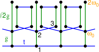
Figure 1: Variational Hilbert space construction for the 1D polaron problem. Basis states are represented by dots, off-diagonal matrix elements by lines. Vertical bonds create or destroy phonons with frequency $\omega_{0}$. Horizontal bonds correspond to electron hops $(\propto t)$. Accordingly, state $|1\rangle$ describes an electron at the origin (0) and no phonon, state $|2\rangle$ is an electron and one phonon both at site 0, $|3\rangle$ is an electron at the nearest-neighbour site 1, and a phonon at site 0, and so on BTB99 .

States in generation $L$ are those obtained by acting $L$ times with these “off-diagonal” terms. Only one copy of each state is retained. Importantly, all translations of these states on an infinite lattice are included. A translation moves the electron and all phonons $j$ sites to the right. Then, according to Bloch’s theorem, each eigenstate can be written as $\psi=\mbox{e}^{{\rm i}kj}a_{L}$, where $a_{L}$ is a set of complex amplitudes related to the states in the unit cell $j$, e.g. $L=7$ for the small variational space shown in Fig. 1. For each momentum $k$ the resulting numerical problem is then to diagonalise a Hermitian $L\times L$ matrix. The total number of states per unit cell ($N_{st}$) after $L$ generations increases exponentially as $(D+1)^{L}$ (note that the bipolaron has the same exponential dependence with only a larger prefactor). Most notably the error in the ground-state energy $E_{0}$ decreases exponentionally, because states are added in a fairly efficient order. Thus in most cases $10^{4}$ – $10^{6}$ basis states are sufficient to obtain an 8-16 digit accuracy for $E_{0}$ (see Fig. 2). The ground-state energy calculated this way is variational for the infinite system.

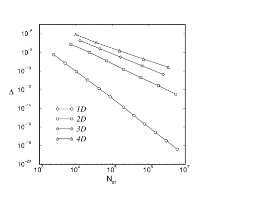
Figure 2: Fractional error $\Delta$ in the ground-state energy of a D-dimensional polaron as a function of the number of basis states $N_{st}$ retained. Parameters are $\lambda=0.5$, $g=1$, and $t=1$. Figure is taken from Ref. KTB02 .

Symmetrisation and phonon truncation

Treating more complex many-particle Hamilton operators on finite lattices, the dimension of the total Hilbert space can also be reduced. To this end we can exploit the space group symmetries [translations ($G_{T}$) and point group operations ($G_{L}$)] and the spin rotational invariance [($G_{S}$); $S^{z}=0~{}$ subspace only]. Working, e.g., on finite 1D or 2D bipartite clusters with periodic boundary conditions (PBC), we do not have all the symmetry properties of the underlying 1D or 2D (square) lattices BWF98 . Restricting ourselves to the 1D non-equivalent irreducible representations of the group $G(\vec{K})=G_{T}\times G_{L}(\vec{K})\times G_{S}$, we can use the projection operator ${\cal P}_{\vec{K},rs}=[g(\vec{K})]^{-1}\sum_{{\cal G}\in G(\vec{K})}\chi_{\vec{K},rs}^{(\cal G)}\;{\cal G}$ (with $[H,{\cal P}_{\vec{K},rs}]=0$, ${\cal P}_{\vec{K},rs}^{\dagger}={\cal P}_{\vec{K},rs}$ and ${\cal P}_{\vec{K},rs}\;{\cal P}_{\vec{K}^{\prime},r^{\prime}s^{\prime}}={\cal P}_{\vec{K},rs}\;\delta_{\vec{K},\vec{K}^{\prime}}\;\delta_{r,r^{\prime}}\;\delta_{s,s^{\prime}}$) in order to generate a new symmetrised basis set: $\{|b\rangle\}\stackrel{{\scriptstyle\cal P}}{{\to}}\{|\tilde{b}\rangle\}$. ${\cal G}$ denotes the $g(\vec{K})$ elements of the group $G(\vec{K})$ and $\chi_{\vec{K},rs}^{(\cal G)}$ is the (complex) character of ${\cal G}$ in the $[\vec{K},rs]$–representation, where $\vec{K}$ refers to one of the $N$ allowed wave vectors in the first Brillouin zone, $r$ labels the irreducible representations of the little group of $\vec{K}$, $G_{L}(\vec{K})$, and $s$ parameterises $G_{S}$. For an efficient parallel implementation of the matrix vector multiplication (see below) it is extremely important that the symmetrised basis can be constructed preserving the tensor product structure of the Hilbert space, i.e.,

$$\{|\tilde{b}\rangle=N^{[\vec{K}rs]}_{\tilde{b}}\,{\cal P}_{\vec{K},rs}\,\left[|\tilde{e}\rangle\otimes|p\rangle\right]\}$$ (6)

with $\tilde{e}=1,\ldots,\tilde{D}_{e}^{g(\vec{K})}$ $[\tilde{D}_{e}^{g(\vec{K})}\sim D_{e}/g(\vec{K})]$. The $N^{[\vec{K}rs]}_{\tilde{b}}$ are normalisation factors.

Since the Hilbert space associated to the phonons is infinite even for a finite system, we use a truncation procedure WRF96 retaining only basis states with at most $M$ phonons:

$$\{|p\rangle\;;\;m_{p}=\sum^{N}_{i=1}m_{i,p}\leq M\}\,.$$ (7)

Then the resulting Hilbert space has a total dimension $\tilde{D}=\tilde{D}_{e}^{g(\vec{K})}\times D_{p}^{M}$ with $D_{p}^{M}=(M+N)!/M!N!$, and a general state of the Holstein model is represented as

$$|\psi_{\vec{K},rs}\rangle=\sum_{\tilde{e}=1}^{\tilde{D}_{e}^{g(\vec{K})}}\sum_{p=1}^{D^{M}_{p}}c_{\tilde{e}p}^{\psi}\,|\tilde{b}\rangle\,.$$ (8)

The computational requirements can be further reduced if one separates the symmetric phonon mode, $B_{0}=\frac{1}{\sqrt{N}}\sum_{i}b_{i}$, and calculates its contribution to $H$ analytically SHBWF05 .

Note that switching from a real space representation to a momentum space description the truncation scheme takes into account all dynamical phonon modes, which has to be contrasted with the frequently used single-mode approach AP98 . In other words, depending on the model parameters and the band filling, the system “decides” by itself how the $M$ phonons will be distributed among the independent Einstein oscillators related to the $N$ Wannier sites or, alternatively, among the different phonon modes in $\vec{Q}$-space. Hence with the same accuracy phonon dynamical effects on lattice distortions being quasi-localised in real space (such as polarons, Frenkel excitons,…) or in momentum space (like charge-density-waves,…) can be studied.

Of course, one has carefully to check for the convergence of the above truncation procedure by calculating the ground-state energy as a function of the cut-off parameter $M$. In the numerical work below convergence is assumed to be achieved if $E_{0}$ is determined with a relative error less than $10^{-6}$ .

Phonon basis optimisation

In this section we outline an advanced phonon optimisation procedure based on controlled density-matrix basis truncation WFWB00 . The method provides a natural way to dress the particles with phonons which allows the use of a very small optimal basis without significant loss of accuracy.

Starting with an arbitrary normalised quantum state,

$$|\psi\rangle=\sum_{e=0}^{D_{e}-1}\sum_{p=0}^{D_{p}-1}c^{\psi}_{ep}[|e\rangle\otimes|p\rangle]\,,$$ (9)

expressed in terms of the basis of the direct product space, we wish to reduce the dimension $D_{p}$ of the phonon space $H_{p}$ by introducing a new basis,

$$|\tilde{p}\rangle=\sum_{p=0}^{D_{p}-1}\alpha_{\tilde{p}p}|p\rangle\,,$$ (10)

with $\tilde{p}=0,\ldots,(D_{\tilde{p}}-1)$ and $D_{\tilde{p}}<D_{p}$. We call $\{|\tilde{p}\rangle\}$ an optimised basis, if the projection of $|\psi\rangle$ on the corresponding subspace $\tilde{H}=H_{e}\otimes H_{\tilde{p}}\subset H$ is as close as possible to the original state. Therefore we minimise

$$\||\psi\rangle-|\tilde{\psi}\rangle\|^{2}=1-{\rm Tr}\;({\bf\alpha\rho\alpha^{\dagger}})$$ (11)

with respect to the $\alpha_{\tilde{p}p}$ under the condition $\langle\tilde{p}^{\prime}|\tilde{p}\rangle=\delta_{\tilde{p}^{\prime}\tilde{p}}$, where

$$|\tilde{\psi}\rangle=\sum_{e=0}^{D_{e}-1}\sum_{\tilde{p}=0}^{D_{\tilde{p}}-1}\sum_{p,p^{\prime}=0}^{D_{p}-1}\alpha_{\tilde{p}p}\alpha_{\tilde{p}p^{\prime}}^{*}c^{\psi}_{p^{\prime}e}[|e\rangle\otimes|p\rangle]$$ (12)

is the projected state. ${\bf\rho}=\sum_{e=0}^{D_{e}-1}(c^{\psi}_{ep})^{*}c^{\psi}_{ep}$ is called the density matrix of the state $|\psi\rangle$. Clearly the states $\{|\tilde{p}\rangle\}$ are optimal if they are elements of the eigenspace of ${\bf\rho}$ corresponding to its $D_{\tilde{p}}$ largest eigenvalues $w_{\tilde{p}}$. If we interpret $w_{\tilde{p}}\sim\exp(-a\tilde{p})$ as the probability of the system to occupy the corresponding optimised state $|\tilde{p}\rangle$, we immediately find that the probability for the complete phonon basis state $\otimes_{i=0}^{N-1}|\tilde{p}_{i}\rangle$ is proportional to $\exp(-a\sum_{i=0}^{N-1}\tilde{p}_{i})$. This is reminiscent of an energy cut-off, and we therefore propose the following choice of a mixed phonon basis $\{|\mu_{i}\rangle\}$ at each site,

$$\forall\ i:\ \{|\mu_{i}\rangle\} = \textrm{ON}(\{|\mu\rangle\})$$ (13)

$$|\mu\rangle = \left\{{\textrm{optimal state }\;\;\;|\tilde{p}\rangle,\ 0\leq\mu<M_{\rm opt}\atop\textrm{bare state }\qquad|p\rangle,\ M_{\rm opt}\leq\mu<M}\right.\,,$$ (14)

and for the complete phonon basis $\left\{\otimes_{\Sigma_{i}\mu_{i}<M}|\mu_{i}\rangle\right\}$, yielding $D_{\rm ph}={N+M-1\choose N}$.

After a first initialisation the optimised states are improved iteratively through the following steps: (1) calculate the requested eigenstate $|\psi\rangle$ of the Hamiltonian $H$ in terms of the actual basis, (2) replace $\{|\tilde{p}\rangle\}$ with the most important (i.e. largest eigenvalues $w_{\tilde{p}}$) eigenstates of the density matrix $\rho$; (3) change the additional states $\{|p\rangle\}$ in the set $\{|\mu\rangle\}$; (4) orthonormalise the set $\{|\mu\rangle\}$, and return to step (1).

A simple way to proceed in step (3) is to sweep the bare states $\{|p\rangle\}$ through a sufficiently large part of the infinite dimensional phonon Hilbert space. One can think of the algorithm as “feeding” the optimised states with bare phonons, thus allowing the optimised states to become increasingly perfect linear combinations of bare phonon states (see Fig. 3).

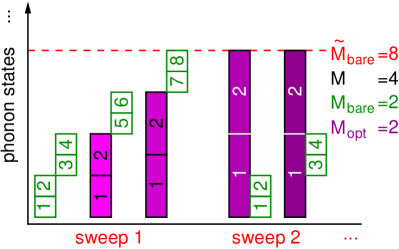
Figure 3: Sweep technique in constructing optimised phonon states.

Solution of the eigenvalue problem

In all the above cases the numerical problem that remains is to find the eigenstates of a (sparse) Hermitian matrix. Here iterative (Krylov) subspace methods like Lanczos CW85 and variants of Davidson Da75 diagonalisation techniques are frequently applied. These algorithms contain basically three steps: (1) project the problem matrix ${\rm A}$ $\in{\rm R}^{n}$ onto a subspace $\bar{\rm A}^{k}\in{\rm V}^{k}$ $(k\ll n)$; (2) solve the eigenvalue problem in ${\rm V}^{k}$ using standard routines; (3) extend the subspace ${\rm V}^{k}\to{\rm V}^{k+1}$ by a vector $\vec{t}\perp{\rm V}^{k}$ and go back to (2). This way we obtain a sequence of approximate inverses of the original matrix ${\rm A}$. A powerful and widely used technique is the Lanczos algorithm which recursively generates a set of orthogonal states (Lanczos vectors):

$$|\varphi_{l+1}\rangle={\rm H}^{\tilde{D}}|\varphi_{l}\rangle-a_{l}|\varphi_{l}\rangle-b_{l}^{2}|\varphi_{l-1}\rangle\,,$$ (15)

where

$$a_{l}=\frac{\langle\varphi_{l}|{\rm H}^{\tilde{D}}|\varphi_{l}\rangle}{\langle\varphi_{l}|\varphi_{l}\rangle}\,,\quad b_{l}^{2}=\frac{\langle\varphi_{l}|\varphi_{l}\rangle}{\langle\varphi_{l-1}|\varphi_{l-1}\rangle}\,,\quad b_{0}^{2}=0\,,$$ (16)

and $|\varphi_{-1}\rangle=0$. Obviously, the representation matrix $[{\rm T}^{L}]_{l,l^{\prime}}=\langle\varphi_{l}|{\rm H}^{\tilde{D}}|\varphi_{l^{\prime}}\rangle$ of ${\rm H}^{\tilde{D}}$ is tridiagonal in the $L$-dimensional Hilbert space spanned by the $\{|\varphi_{l}\rangle\}_{l=0,\ldots,L-1}$, where $L\ll\tilde{D}$. The eigenvalue spectrum of ${\rm T}^{L}$ can be easily determined using standard routines from libraries such as EISPACK (see http://www.netlib.org). Note that the convergence of the Lanczos algorithm is excellent at the edges of the spectrum (the ground state for example is obtained with high precision after at most $\sim 100$ Lanczos iterations) but rapidly worsens inside the spectrum.

In general the computational requirements of these eigenvalue algorithms are determined by matrix-vector multiplications (MVM), which have to be implemented in a parallel, fast and memory saving way on modern supercomputers. The MVM step can be be done in parallel by using a parallel library such as PETSc (see http://www-unix.mcs.anl.gov/petsc/petsc-as/).

Our matrices are extremely sparse because the number of non-zero entries per row of our Hamilton matrix scales linearly with the number of electrons. Therefore a standard implementation of the MVM step uses a sparse storage format for the matrix, holding the non-zero elements only. The typical storage requirement per non-zero entry is 12-16 Byte, i.e. for a matrix dimension of $\tilde{D}=10^{9}$ about one TByte main memory is required to store only the matrix elements of the EP Hamiltonian. To extend our EP studies to even larger matrix sizes we no longer store the non-zero matrix elements but generate them in each MVM step. Of course, at that point standard libraries are no longer useful and a parallel code tailored to each specific class of Hamiltonians must be developed. Clearly the parallelisation approach follows the inherent natural parallelism of the Hilbert space. Assuming that the electronic dimension ($\tilde{D}_{e}$) is a multiple of the number of processors used we can easily distribute the electronic basis states among the processors. As a consequence of this choice only the electronic hopping term generates inter-processor communication in the MVM while all other (diagonal electronic) contributions can be computed locally on each processor. Using supercomputers with hundreds of processors and one TByte of main memory, such as the IBM p690 cluster, at the moment, one is able to run simulations up to a matrix dimension of $3\times 10^{10}$.

Determination of dynamical correlation functions

The numerical calculation of dynamical spectral functions,

$$A^{\cal O}(\omega) = -\lim_{\eta\to 0^{+}}\frac{1}{\pi}\mbox{Im}\left[\langle\psi_{0}|{\rm O}^{\dagger}\frac{1}{\omega-{\rm H}+E_{0}+i\eta}{\rm O}|\psi_{0}\rangle\right]$$ (17)

$$= \sum_{n=0}^{\tilde{D}-1}|\langle\psi_{n}|{\rm O}|\psi_{0}\rangle|^{2}\delta[\omega-(E_{n}-E_{0})]\,,$$

where ${\rm O}$ is the matrix representation of a certain operator ${\cal O}$ [e.g., the creation operator $c_{\vec{K}}^{\dagger}$ of an electron with wavevector $\vec{K}$ if one wants to calculate the single-particle spectral function; or the current operator $\hat{\jmath}=-\mbox{i}et\sum_{i}(c_{i}^{\dagger}c_{i+1}-c_{i+1}^{\dagger}c_{i})$ if one is interested in the optical conductivity], involves the resolvent of the Hamilton matrix ${\rm H}$. Once we have obtained the eigenvalues and eigenvectors of $H$ we can plug them into Eq. (17) and directly obtain the corresponding dynamical correlation or Green functions. For the typical EP problems under investigation we deal with Hilbert spaces having total dimensions $\tilde{D}$ of $10^{6}$ - $10^{11}$. Finding all eigenvectors and eigenstates of such huge Hamilton matrices is impossible, because the CPU time required for exact diagonalisation of ${\rm H}$ scales as $\tilde{D}^{3}$ and memory as $\tilde{D}^{2}$. So in practice this “naive” approach is applicable for small Hilbert spaces only, where the complete diagonalisation of the Hamilton matrix is feasible. Fortunately, there exist very accurate and well-conditioned linear scaling algorithms for a direct approximate calculation of $A^{\cal O}(\omega)$.

Kernel polynomial method (KPM)

The idea of the KPM (for a review see WWAF06 ), is to expand $A^{\cal O}(\omega)$ in a finite series of $L+1$ Chebyshev polynomials $T_{m}(x)=\cos[m\arccos(x)]$. Since the Chebyshev polynomials are defined on the real interval $[-1,1]$, first a simple linear transformation to the Hamiltonian and all energy scales has to be applied: ${\rm X}=({\rm H}-b)/a$, $x=(\omega-b)/a$, $a=(E_{max}-E_{min})/2(1-\epsilon)$, and $b=(E_{max}+E_{min})/2$ (the small constant $\epsilon$ is introduced in order to avoid convergence problems at the endpoints of the interval – a typical choice is $\epsilon\sim 0.01$ which has only 1% impact on the energy resolution SR97 ). Then the expansion is

$$A^{\cal O}(x)=\frac{1}{\pi\sqrt{1-x^{2}}}\left(\mu_{0}^{\cal O}+2\sum_{m=1}^{L}\mu_{m}^{\cal O}T_{m}(x)\right)\,,$$ (18)

with moments

$$\mu_{m}^{\cal O}=\int_{-1}^{1}dx\,T_{m}(x)A^{\cal O}(x)=\langle\psi_{0}|{\rm O}^{\dagger}T_{m}({\rm X}){\rm O}|\psi_{0}\rangle\,.$$ (19)

Eq. (18) converges to the correct function for $L\to\infty$. The moments

$$\mu_{2m}^{\cal O}=2\langle\phi_{m}|\phi_{m}\rangle-\mu_{0}^{\cal O}\quad\mbox{and}\quad\mu_{2m+1}^{\cal O}=2\langle\phi_{m+1}|\phi_{m}\rangle-\mu_{1}^{\cal O}$$ (20)

can be efficiently obtained by repeated parallelised MVM, where $|\phi_{m+1}\rangle=2{\rm X}|\phi_{m}\rangle-|\phi_{m-1}\rangle$ but now $|\phi_{1}\rangle={\rm X}|{\rm O}\phi_{0}\rangle$ with $|\phi_{0}\rangle\equiv|\psi_{0}\rangle$ determined by Lanczos ED.

As is well known from Fourier expansion, the series (18) with $L$ finite suffers from rapid oscillations (Gibbs phenomenon) leading to a poor approximation to $A^{\cal O}(\omega)$. To improve the approximation the moments $\mu_{n}$ are modified $\mu_{n}\to g_{n}\mu_{n}$, where the damping factors $g_{n}$ are chosen to give the “best” approximation for a given $L$. In more abstract terms this truncation of the infinite series to order $L$ together with the corresponding modification of the coefficients is equivalent to a convolution of the spectral function with a smooth approximation kernel $K_{L}(x,y)$. The appropriate (optimal) choice of this kernel, that is of $g_{n}$, e.g. to guarantee positivity of $A^{\cal O}(\omega)$, lies at the heart of KPM. We mainly use the Jackson kernel which results in a uniform approximation whose resolution increases as $1/L$, but for the determination of the single-particle Green functions below we use a Lorentz kernel which mimics a finite imaginary part $\eta$ in Eq. (17) WWAF06 .

In view of the uniform convergence of the expansion, the accuracy of the spectral functions can be made as good as required by just increasing $L$.

Cluster perturbation theory (CPT)

The spectrum of a finite system of $N$ sites which we obtain through KPM differs in many respects from that in the thermodynamic limit $N\to\infty$, especially in that it is obtained for a finite number of momenta $K=\pi\,m/N$ only. While we cannot easily increase $N$ without going beyond computationally accessible Hilbert spaces we can try to extrapolate from a finite to the infinite system.

For this purpose we first calculate the Green function $G^{c}_{ij}(\omega)$ for all sites $i,j=1,\dots,N_{c}$ of a $N_{c}$ – size cluster with open boundary conditions, and then recover the infinite lattice by pasting identical copies of this cluster at their edges SPP00 . The “glue” is the hopping $V$ between these clusters, where $V_{kl}=t$ for $|k-l|=1$ and $k,l\equiv 0,1({\rm mod}N)$, which is dealt with in first order perturbation theory. Then the Green function $G_{ij}(\omega)$ of the infinite lattice is given through a Dyson equation $G_{ij}(\omega)=G^{c}_{ij}(\omega)+\sum_{kl}G^{c}_{ik}(\omega)V_{kl}G_{lj}(\omega)$, where indices of $G^{c}(\omega)$ are counted modulo $N_{c}$. The Dyson equation is solved by Fourier transformation over momenta $K=kN_{c}$ corresponding to translations by $N_{c}$ sites

$$G_{ij}(K,\omega)=\left[\frac{G^{c}(\omega)}{1-V(K)G^{c}(\omega)}\right]_{ij}\,,$$ (21)

from which one finally obtains

$$G(k,\omega)=\frac{1}{N_{c}}\sum_{i,j=1}^{N_{c}}G^{c}_{ij}(N_{c}k,\omega)\exp(-\mathrm{i}k(i-j))\;.$$ (22)

In this way we obtain a Green function $G(k,\omega)$ with continuous momenta $k$ from the cluster Green function $G^{c}$. Two approximations are made, one by using first order perturbation theory in $V=t$, the second on assuming translational symmetry in $G_{ij}(\omega)$ which is only approximatively satisfied.

3 Ground state results

The VED method can compute polaron properties in dimensions 1 through 4 and higher. The energies for 1D to 4D polarons at $\vec{k}=0$ for intermediate to weak coupling on linear, square, cubic, and hypercubic lattices are listed in the Tab. LABEL:t:e0. The number of significant digits is determined by comparing the energy as the size of the Hilbert space is increased. The accuracy is high compared to that of other numerical methods, even when limited by the single-processor desktop workstations of several years ago, on which the results were obtained KTB02 . Correlation functions are generally less accurate than energies.

Table 1: Polaron ground state energies at $\vec{k}=0$ in 1D - 4D for $\lambda=0.5$ and $g=1.0$ In the following $t=1$ unless specifically noted.

	1D	2D	3D	4D
$E_{0}/t\quad$	-2.46968472393287071561	-4.814735778337	-7.1623948409	-9.513174069

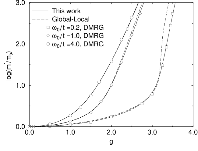
Figure 4: Logarithm of the polaron effective mass in 1D as a function of $g$. VED results (full lines) were obtained operating repeatedly $L=20~{}$ times with the off-diagonal pieces of the Holstein Hamiltonian (cf. Sec. 2.2). For comparison GL (global-local) results (dashed lines) are included RBL98 . Open symbols, indicating the value of $\omega_{0}/t$, are DMRG results JW98b .

Figure 4 shows the effective mass computed by VED BTB99 in comparison with GL and DMRG methods. $m^{*}$ is obtained from

$${m_{0}\over m^{*}}=\left.{1\over{2t}}{\partial^{2}E_{k}\over{\partial k^{2}}}\right|_{k=0},$$ (23)

where $m_{0}=1/(2t)$ is the effective mass of a free electron. The second derivative is evaluated by small finite differences in the neighbourhood of ${\vec{k}}=0$. Note that although the calculated energy $E_{\vec{k}}$ is a variational bound for the exact energy, there is no such control on the mass, which may be either above or below the exact answer, and is expected to be more difficult to obtain accurately. Nevertheless, in the intermediate coupling regime where VED at $L=20$ gives an energy accuracy of 12 decimal places, one can calculate the effective mass accurately (6-8 decimal places) by letting $\Delta k\to 0$.

In Fig. 4 the parameters span different physical regimes including weak and strong coupling, and low and high phonon frequency. We find good agreement between VED and GL away from strong coupling and excellent agreement in all regimes with DMRG results. DMRG calculations are not based on finite-$k$ calculations due to a lack of periodic boundary conditions, so they extrapolate the effective mass from the ground state data using chains of different sizes, which leads to larger error bars and demands more computational effort. Notice that their discrete data is slightly scattered around the VED curves. Nevertheless, both methods agree well. We have compared the VED results for effective mass obtained on different systems from $L=16$ with $N_{st}=178617$ states to $L=20$ with $N_{st}=2975104$ states and obtained convergence of results to at least 4 decimal places in all parameter regimes presented in Fig. 4. Our error is therefore well below the linewidth. Even though there is no phase transition in the ground state of the model, the polaron becomes extremely heavy in the strong coupling regime. The crossover to a regime of large polaron mass is more rapid in adiabatic regime, i.e. at small $\omega_{0}/t$.

The polaron effective mass in higher dimensions is shown as a function of the EP coupling in Fig. 5. The mass increases exponentially for large $\lambda$. The crossover to larger effective mass is more rapid, though still continuous, in higher dimensions.

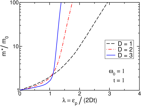
Figure 5: Effective mass of the Holstein polaron in dimensions 1, 2, and 3.

Of course it is of special interest to understand the evolution of the polaronic band structure as the EP coupling strength increases. Figure 6 presents the results for the wavevector dependence of the ground-state energy $E_{k}$ in 1D at weak (a) and strong (b) EP couplings.

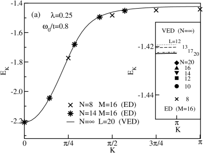
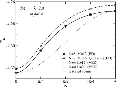
Figure 6: Band structure of the 1D Holstein model in the weak (a) and strong (b) EP coupling regimes. $M$ and $L$ denote the number of phonons and the depth of the basis in ED and VED calculations, respectively. Within ED the ($Q=0$) centre of mass motion has been separated if indicated. The inset shows the finite-size dependence being significant for weak EP coupling only. In the strong EP coupling case ED results basically agree with those obtained by VED.

As might be expected, for $\lambda=0.25$ the coherent bandwidth, $\Delta E=\sup_{k}E_{k}-\inf_{k}E_{k}$, is approximately given by the phonon energy ($\Delta E=0.782\sim\omega_{0}=0.8$). If the EP interaction is enhanced a band collapse appears. Note, however, that even in the relatively strong EP coupling regime displayed Fig. 6 (b) the standard Lang-Firsov formula, $\Delta E_{LF}=4Dt\exp[-g^{2}]$ (obtained by performing the Lang-Firsov canonical transformation LF62 and taking the expectation value of the kinetic energy over the transformed phonon vacuum), does not give a satisfactory estimate of the bandwidth. So we found $\Delta E_{LF}=0.0269$ which has to be contrasted with the exact result $\Delta E=0.0579$. Besides the band narrowing effect, there are several other features worth mentioning for polaronic band states in the crossover region. Most notably, throughout the whole Brillouin zone the band structure differs significantly from that of a rescaled tight-binding (cosine) band containing only nearest-neighbour hopping WF97 . Obviously the residual polaron-phonon interaction generates longer-ranged hopping processes Fi75 ; WF97 . Concomitantly, the mass enhancement due to the EP interaction is weakened at the band minimum. It is important to realize that these effects are most pronounced at intermediate EP couplings and phonon frequencies. In this parameter region even higher-order strong-coupling perturbation theory, with its internal states containing some excited phonons, seems to be intractable because the convergence of the series expansion is poor St96 . Of course the dispersion is barely changed from a rescaled tight-binding band in the very extreme small polaron limit ($\lambda,\;g^{2}\gg 1$).

Further information about the quasiparticle may be obtained by computing the quasiparticle residue, the overlap squared between a bare electron and a polaron,

$$Z_{\vec{k}}=|\langle\psi_{\vec{k}}|c_{\vec{k}}^{\dagger}|0\rangle|^{2},$$ (24)

where $|0\rangle$ is the state with no electron and no phonon excitations, and $|\psi_{\vec{k}}\rangle$ is the polaron wavefunction at momentum $\vec{k}$. $Z_{\vec{k}}$ can be measured by angle-resolved photoemission, and gives the bare electronic contribution of the polaronic state. The phonon contribution to the quasiparticle is described by the $k-$dependent mean phonon number

$$N^{ph}_{\vec{k}}=\sum_{i}|\langle\psi_{\vec{k}}|b_{i}^{\dagger}b_{i}|\psi_{\vec{k}}\rangle|^{2}.$$ (25)

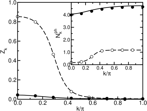
Figure 7: The quasiparticle weight $Z_{\vec{k}}$ and in the inset the total number of phonons $N^{ph}_{\vec{k}}$ as a function of the wavevector ${\vec{k}}$ for the 1D Holstein model with $(\bar{g}/t)^{2}=0.4$ [dashed line (VED); open circles (ED)], $3.2$ [solid line (VED); filled circles (ED)]. $\alpha=\omega_{0}/t=0.8.$ Data are taken from Refs. BTB99 ; WF97 .

Figure 7 shows the spectral weight $Z_{\vec{k}}$ and the mean phonon number $N_{\vec{k}}^{ph}$ as a function of $\vec{k}$. The two sets of parameters correspond to the large and small polaron regime respectively. The DMRG cannot straightforwardly compute this quantity. There is excellent agreement between the VED and ED methods in the weak coupling case. In the strong coupling regime there is an approximately $1\%$ disagreement in $N^{ph}_{\vec{k}}$ due to a lack of phonon degrees of freedom in the variational space of the ED calculation. The results in the weak coupling case show a smooth crossover from predominantly electronic character of the wavefunction for small $k$ (large $Z_{\vec{k}}$ and small $N^{ph}_{\vec{k}}\approx 0$) to predominantly phonon character around ${\vec{k}}=\pi$ characterised by $Z_{\vec{k}}\approx 0$ and $N^{ph}_{\vec{k}}\approx 1$. In the strong coupling regime there is less $\vec{k}$-dependence. The $Z_{\vec{k}}$ is already close to zero at small $k$, indicating strong EP interactions that lead to a large polaron mass. Concomitantly an appropriately defined polaron quasiparticle residue $\tilde{Z}_{0}$ tends to one FLW97 ; LHF06 . So we arrive at the conclusion that a well-defined electronic (polaronic) quasiparticle exists for $k=0$ at weak (strong) EP coupling.

VED is one of the few methods that can also calculate the polaron band dispersion in 3D systems (QMC is another, but is limited to the condition that the polaron bandwidth is much smaller than the phonon frequency, which corresponds to the strong-coupling regime.) Figure 8(a) shows the band dispersion for the 3D polaron along symmetry directions in the Brillouin zone at various EP coupling constants $\bar{g}=g\omega_{0}$.

Figure 8: Ground-state energy $E_{\vec{k}}$ (shifted by $E_{0}$) of the 3D polaron in panel (a) and quasiparticle weight $Z_{\vec{k}}$ in panel (b) for three different EP coupling constants, $\bar{g}=4.5$ (solid line), $\bar{g}=3.5$ (dotted line), and $\bar{g}=2.0$ (dashed line), for $\omega_{0}/t=2$. The dot-dashed line in (a) is the dispersion of a bare electron. The corresponding ground state energies $E_{0}/t$ are $-10.608348,\;-8.0642850$, and $-6.588526818$ respectively.

Starting with weak coupling $\bar{g}=2.0$ (dashed line), the polaron band is close to the bare electron band at the lower band edge. The deviation between them increases as ${\vec{k}}$ increases. When $E_{\vec{k}}-E_{0}$ approaches $\omega_{0}$, we observe a band flattening effect, similar to the 1D and 2D cases, accompanied by a sharp drop of quasiparticle weight $Z_{\vec{k}}$ (see Fig. 8(b)). The large $\vec{k}$ lowest energy state can be considered roughly as “a $\vec{k}=0$ polaron ground state” plus “an itinerant (or weakly-bound) phonon with momentum ${\vec{k}}$”. It is the phonon that carries the momentum so as to make $Z_{\vec{k}}$ essentially vanish and give an approximate bandwidth $\omega_{0}$. Due to the large spatial extent of the EP correlations in the flattened band, our results are less accurate in this regime. In the case of intermediate coupling $\bar{g}=3.5$ ($\lambda=1.0208$), the polaron bandwidth is narrower than the phonon frequency. The upper part of the band has much less dispersion than the lower part but with a substantial $Z_{\vec{k}}$. This indicates a distinct mechanism for the crossover as a function of ${\vec{k}}$. In the case of $\bar{g}=4.5$, the strong EP interaction leads to a significant suppression of $Z_{\vec{k}}$ at all ${\vec{k}}$. $Z_{\vec{k}=0}$ approaches the strong-coupling result $Z=\exp(-g^{2})$ for $\lambda\,,g^{2}\gg 1$. Note that the inverse effective mass $m^{*}/m_{0}$ and $Z$ differ if the self-energy is strongly ${\vec{k}}$-dependent. This discrepancy has its maximum in the intermediate-coupling regime for 1D systems, but vanishes in the limit $\lambda\to\infty$. In the Holstein model with on-site electron-phonon interactions, $Z$ and the inverse effective mass are closely related. However, the two can be made arbitrarily different by increasing the range of the EP interaction KTB02 .

The correlation function between the electron position and the phonon displacement is

$$\chi_{i,j}=\langle\psi_{\vec{k}}|c_{i}^{\dagger}c_{i}(b_{j}+b^{\dagger}_{j})|\psi_{\vec{k}}\rangle.$$ (26)

This correlation function can be considered as a measure of the polaron size. It should not be confused with the “polaron radius” in the extreme adiabatic limit, which refers to the spatial extent of a hypothetical symmetry-breaking localised state. The ground-state EP correlation function is plotted for the 1D Holstein polaron in Fig. 9.

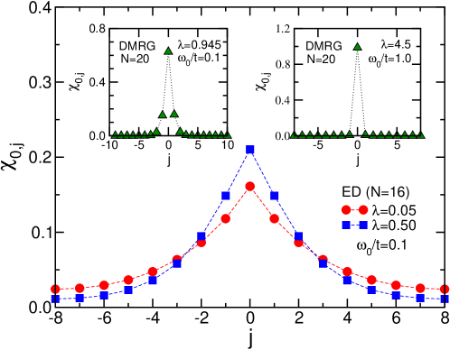
Figure 9: Renormalised EP correlation function $\chi_{0,j}=\langle n_{0}(b^{\dagger}_{0+j}+b_{0+j})\rangle/2g\langle n_{0}\rangle$ as a function of the electron-phonon separation $j$ in the $\vec{k}=0$ ground state of the 1D Holstein model. Results are taken from WF98a ; FAHW06 .

For parameters close to the (adiabatic) weak EP coupling regime (main panel), the amplitude of $\chi_{0,j}$ is small and the spatial extent of the electron-induced lattice deformation is spread over the whole (finite) lattice. The DMRG results shown in the left inset indicate a substantial reduction of the polaron’s size near the crossover region. Finally a small polaron is formed at large couplings (right inset); now the position of the electron and the phonon displacement is strongly correlated.

How does the electron-phonon correlation function change as the polaron acquires a nonzero momentum $\vec{k}$? The answer is shown for 1D in Fig. 10 BTB99 . The parameters correspond to weak coupling. At $k=0$, where the group velocity is zero, the deformation is limited to only a few lattice sites around the electron. The correlation is always positive and exponentially decaying. At finite but small $k=\pi/4$, the deformation around the electron increases in amplitude and rings (oscillates in sign) as the polaron acquires a finite group velocity. At $k=\pi/2$ the ringing is strongly enhanced. Note also that the spatial extent of the deformation increases in comparison to $k=0$. The range of the deformation is maximum at $k=\pi$, where it extends over the entire region shown in the figure. In keeping with the larger extent of the lattice deformation near $k=\pi$, the ground-state energy $E_{\pi}$ converges more slowly with the size of the Hilbert space. We have also computed the $k-$dependent $\chi$ for the strong-coupling case $\omega_{0}=0.8,\bar{g}^{2}=3.2$ (not shown). We find only weak $k-$dependence, which is a consequence of the crossover to the small polaron regime. The lattice deformation is localised predominantly on the electron site.

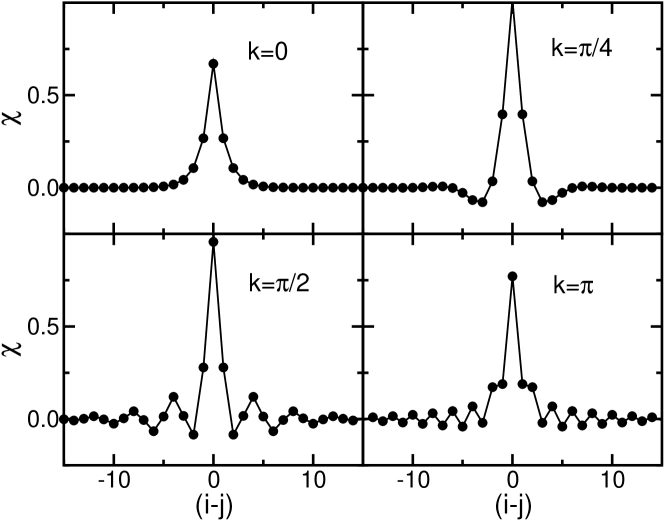
Figure 10: Lattice deformation $\chi$ for 1D as a function of $(i-j)$ for $\omega_{0}=0.8$, $t=1$, $\bar{g}^{2}=0.4$ and $L=18$, for four different values of momentum $k$. The variational Hilbert space for $L=18$ allows nonzero correlations up to a maximum distance $|i-j|_{max}=17$. Only distances up to 15 are plotted.

Over four decades ago, a simple and intuitive variational approach to the 1D polaron problem was proposed by Toyozawa To61 . This method has been successfully applied to various fields and revisited in a number of guises over the years. It is generally believed to provide a qualitatively correct description of the polaron ground state, aside from predicting a spurious discontinuous change in the mass at intermediate coupling. The Toyozawa variational wavefunction consists of a product of coherent states (displaced oscillators) around the instantaneous electron position. The phonons create a symmetrical cloud around the electron. Numerical studies of the 1D electron-phonon correlation function (two-point function) are in semi-quantitative agreement with the Toyozawa variational wavefunction. The numerically exact three-point function, however, disagrees wildly. Denoting the instantaneous electron position as 0, the Toyozwa variational wavefunction requires that the probability to find phonon excitations, for example, on both sites 3 and 4, should be identical to finding them on sites (-3) and 4. Numerically, however, the latter is many orders of magnitude less probable KTB02 . This suggests a physical picture in which the $k=0$ polaron is viewed not as an electron surrounded by a symmetrical cloud of phonons, but is instead a coherent superposition of two “comets,” one with a tail extending to the right, and the other to the left.

Figure 11: On-site correlation $\chi(0)$ for the 3D polaron. VED results (solid lines) KTB02 are compared to DMFT (dotted lines with symbols) CPFF97 . $\chi(0)$ is normalised to 1 when $\lambda$ is infinite (i.e. $t\to 0$) according to $\mathop{\lim}\limits_{t\to 0}\chi(0)=2g$. Parameters are $\omega_{0}=t=1$.

Studying the properties of Holstein polarons, DMFT is exact in infinite dimensions. An interpolation to 3D lattices is made possible by using a semielliptical free density of states $N(E)$ to mimic the low-energy features. Here DMFT is accurate in the strong-coupling regime, where the surrounding phonons are predominately on the electron site. This is also the regime where strong-coupling perturbation theory works well. However, DMFT fails to compute quantities such as the polaron mass correctly in the weak-coupling regime. The reason is that in DMFT, the lattice problem is mapped onto a self-consistent local impurity model, which preserves the interplay of the electron and the phonons only at the local level. The spatial extent of the EP correlations increases as the EP coupling decreases, which explains the significant discrepancy in the weak-coupling regime. Therefore only the on-site EP correlation has been studied by DMFT, and the results are compared with VED KTB02 in Fig. 11. There is good qualitative agreement. The curves show a rapid change in slope only for large $g$, where DMFT is less accurate. It is worth noting that DMFT neglects the $\vec{k}$ dependence of self-energy, i.e., the inverse effective mass is always equal to the quasiparticle spectral weight. Clearly the difference between $m_{0}/m^{*}$ and the spectral weight $Z_{\vec{k}}$ is not negligible in the intermediate- to weak-coupling regime.

4 Excited states

In this section we turn our attention from the ground state to the excited states of the Holstein model. Figure 12 plots the energy eigenvalues for a small variational space containing a maximum of 9 phonon excitations. The lowest curve is the polaron ground state at momentum $k$. Excited states are the polaron with additional bound or unbound (or both) phonon excitations. A ripple can be discerned near the bare electron dispersion. The figure superficially resembles a “band structure,” which however encodes ground and excited state information for the many-body (many phonon) polaron problem. The ac conductivity of the polaron, for example, appears as an “interband” transition in this mapping.

Figure 12: The ground and excited state 1D polaron energy eigenvalues (those energies below 0) are plotted as a function of $k$ (in units of $\pi$) for $\bar{g}=\omega_{0}=t=1$, $L=9$, $N_{st}=1185$.

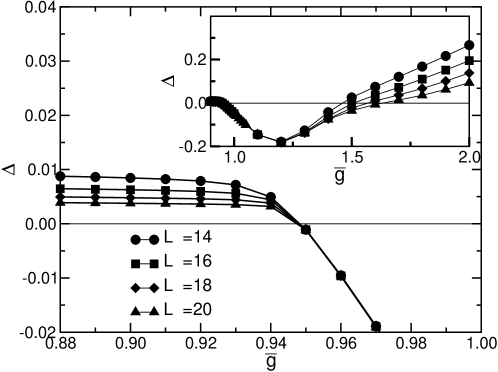
Figure 13: First excited state binding energy $\Delta=E_{1}-E_{0}-\omega_{0}$ as a function of $\bar{g}~{}$ BTB99 . Results are for $\omega_{0}=0.5$ and various Hilbert space sizes $L$. Inset: Binding energy over a wider range of $\bar{g}$.

What is the nature of the first excited state? We focus on the question of whether an extra phonon excitation forms a bound state with the polaron, or instead remain as two widely separated entities. Using numerical and analytical approaches we show evidence that there is a sharp phase transition (not a crossover) between these two types of states, with a bound excited state appearing only as the EP coupling is increased. Although the ground state energy $E_{0}$ is an analytic function of the parameters in the Hamiltonian, there are points at which the energy $E_{1}$ of the first excited state is nonanalytic. In previous work, Gogolin has found bound states of the polaron and additional phonon(s), but he does not obtain a phase transition between bound and unbound states because his approximations are limited to strong coupling $g\gg 1$ Go82 . A phase transition between a bound and unbound first excited state has been calculated for 3D using a dynamical CPA (coherent potential approximation) Su74 and DMFT CPFF97 .

We compute the energy difference $\Delta E=E_{1}-E_{0}$, where $E_{1}$ and $E_{0}$ are the first excited state and the ground state energies at $k=0$ (the two lowest bands in Fig. 12). In the case where the first excited state of a polaron can be described as a polaron ground state and an unbound extra phonon excitation, this energy difference should in the thermodynamic limit equal the phonon frequency, $\Delta E=\omega_{0}$. In Fig. 13 we plot the binding energy $\Delta=\Delta E-\omega_{0}$ for $\omega_{0}=0.5$ as a function of the EP coupling $\bar{g}$ for various sizes of the variational space. We see two distinct regimes. Below $\bar{g}_{c}\sim 0.95$, $\Delta$ varies with the system size but remains positive $(\Delta>0)$. Physically, for $\bar{g}<\bar{g}_{c}$, the additional phonon excitation would prefer to be infinitely separated from the polaron, but is confined to a distance no greater than $L-1$ by the variational Hilbert space. As the system size increases, $\Delta$ slowly approaches zero from above as the “particle in a box” confinement energy decreases. In the other regime, $\bar{g}>\bar{g}_{c}$, the data has clearly converged and $\Delta<0$. This is the regime where the extra phonon excitation is absorbed by the polaron forming an excited polaron bound state. Since the excited polaron forms an exponentially decaying bound state, the method already converges at $L=14$. In the inset of Fig. 13 we show the binding energy $\Delta$ in a larger interval of EP coupling $\bar{g}$. Although the results cease to converge at larger $\bar{g}$, we notice that the binding energy $\Delta$ reaches a minimum as a function of $\bar{g}$. As one can demonstrate within the strong coupling approximation, the true binding energy approaches zero exponentially from below with increasing $\bar{g}$.

Figure 14 shows the phase diagram for $k=0$ separating the two regimes. The phase boundary, given by $\Delta=0$, was obtained numerically, and compared to strong coupling perturbation theory in $t$ to first and second order. The phase transition where $\Delta$ becomes negative at sufficiently large $\bar{g}$ is also seen in ED calculations.

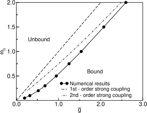
Figure 14: The phase diagram for the bound to unbound transition of the first excited state, obtained using the condition $\Delta(\omega_{0},\bar{g})=0$. The corresponding phase diagram for the ground state would be blank: there is no phase transition in the ground state, only a crossover.

The distribution of the number of phonons in the vicinity of the electron is defined as

$$\gamma(i-j)=\langle\psi_{k}|c_{i}^{\dagger}c_{i}b^{\dagger}_{j}b_{j}|\psi_{k}\rangle.$$ (27)

In Fig. 15 we compute this distribution for the ground state $\gamma_{0}$ and the first excited state $\gamma_{1}$ slightly below $(\bar{g}=0.9)$, and above $(\bar{g}=1.0)$ the transition for $\omega_{0}=0.5$.

The central peak of the correlation function $\gamma_{1}$ below the transition point is comparable in magnitude to $\gamma_{0}$ (Fig. 15 (a,b)). The main difference between the two curves is the long range decay of $\gamma_{1}$ as a function of distance from the electron, onto which the central peak is superimposed. The extra phonon that is represented by this long-range tail extends throughout the whole system and is not bound to the polaron. The existence of an unbound, free phonon is confirmed by computing the difference of total phonon number $N^{ph}_{0,1}=\sum_{l}\gamma_{0,1}(l)$. This difference should equal one below the transition point. Our numerical values give $N^{ph}_{1}-N^{ph}_{0}\sim 1.02$. We attribute the deviation from the exact result to the finite relative separation allowed.

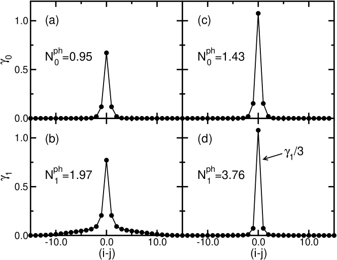
Figure 15: The phonon number $\gamma$ as a function of the distance from the electron position for the ground state (a) and the first excited state (b), both computed at $\bar{g}=0.9$; and the same in (c) and (d) for $\bar{g}=1.0$. All data are computed at phonon frequency $\omega_{0}=0.5$ and $L=18$. Note that (d) is a plot of $\gamma_{1}/3$. In (a,b), $\gamma_{1}-\gamma_{0}$ drops to zero around $|i-j|=15$. This is a finite-size effect. Computing the same quantity with larger $L$ below the phase transition would lead to a larger extent of the correlation function indicating that the extra phonon excitation is not bound to the polaron.

Correlation functions above the transition point (Fig. 15 (c,d)) are physically different. First, phonon correlations in $\gamma_{1}$ decay exponentially, which also explains why the convergence in this region is excellent. Second, the size of the central peak in $\gamma_{1}$ is 3 times higher than $\gamma_{0}$. (Note that to match scales in Fig. 15 (d) we divided $\gamma_{1}$ by 3). The difference in total phonon number gives $N^{ph}_{1}-N^{ph}_{0}\sim 2.33$. We are thus facing a totally different physical picture: The excited state is composed of a polaron which contains several extra phonon excitations (in comparison to the ground-state polaron) and the binding energy of the excited polaron is $\Delta<0$. The extra phonon excitations are located almost entirely on the electron site. The value of $\gamma_{1}-\gamma_{0}$ at $j=0$ is 2.16, which almost exhausts the phonon sum.

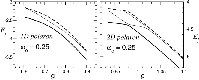
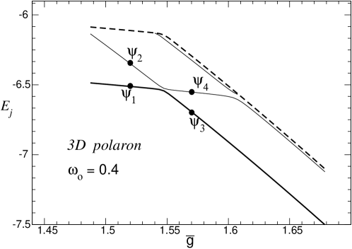
Figure 16: Eigenvalues of low-lying states as functions of coupling constant in 1D through 3D. Hopping $t=1$ in all panels. In the adiabatic regime in higher dimensions, the ground state (thick solid lines) shows a fairly abrupt change in slope. In the 3D panel, $\psi_{1}$ and $\psi_{4}$ are a lightly-dressed electron state; $\psi_{2}$ and $\psi_{3}$ are a heavy polaron state. The dashed lines are the beginning of the lowest continua.

Next we discuss the role of dimensionality in the excited states. The effect of dimensionality on static properties has been studied previously EH76 ; JE83 ; KM93 ; KTB02 . The eigenvalues of the low-lying $k=0$ states are shown as functions of $\bar{g}$ in Fig. 16. The energy spectra in D$>$1 are qualitatively different than in 1D. The 1D polaron ground state becomes heavy gradually as $\bar{g}$ increases. However, in D$\geq$2, the ground state crosses over to a heavy polaron state by a narrow avoided level crossing, which is consistent with the existence of a potential barrier EH76 . In the lower panel of Fig. 16, $\psi_{1}$ and $\psi_{4}$ are nearly free electron states; $\psi_{2}$ and $\psi_{3}$ are heavy polaron states. The inner product $|\langle\psi_{1}|\psi_{4}\rangle|$ is equal to 0.99. Just right of the crossing region the effective mass (approximately equal to the inverse of the spectral weight) of the first excited state can be smaller than the ground state by 2 or 3 orders of magnitude, while their energies can differ by much less than $\omega_{0}$. The narrow avoided crossing description works less well for larger $\omega_{0}$.

5 Dynamics of polaron formation

How does a bare electron time evolve to become a polaron quasiparticle? The bare electron can be injected by inverse photoemission or tunnelling, or a hole by photoemission, or an exciton (electron-hole bound state) by fast optics.

One approach is to construct a variational many-body Hilbert space including multiple phonon excitations, and to numerically integrate the many-body Schrödinger equation,

$$i{{d\psi}\over{dt}}=H\psi$$ (28)

in this space KG96 . The full many-body wave function is obtained. This method includes the full quantum dynamics of the electrons and phonons. Note that alternative treatments, such as the semiclassical approximation that treats the phonons classically, fail for this problem, particularly in the limit of a wide initial electron wavepacket.

Figure 17 shows snapshots of polaron formation at weak coupling. An initial bare electron wave packet is launched to the right as shown in panel (a). This initial condition is relevant to the recent experiments Geea98 ; SSKYK01 ; DVBS00 ; TNSSTK98 ; AT02 , and to electron injection from a time-resolved STM (scanning tunneling microscope) tip DRT00 . Although polarons injected optically or by STM can have a range of initial momenta, it would be more realistic to take $k=0$ for an optically created exciton. In panel (b) the electron is not yet dressed and thus is moving roughly as fast as the free electron (green dashed line). In addition, there exists a back-scattered current (which later evolves into a left-moving polaron) on the left side of the wave packet (green dot-dashed and thick black curves). In panel (c) after an elapsed time of one phonon period, the electron density consists of two peaks. The peak on the right (black arrow) is essentially a bare electron. The peak on the left is a polaron wave packet moving more slowly. As time goes on, the bare electron peak decays and the polaron peak grows. Some phonons are left behind (blue double-dot dashed line), mainly near the injection point. These phonons are of known phase with displacement shown in thin solid red. Some phonon excitations travel with the polaron (magenta dot double-dashed line). Finally, a coherent polaron wave packet is observed when the polaron separates from the uncorrelated phonon excitations. The velocity operator is defined as

$$\hat{v}_{j}\equiv{2\hat{\jmath}_{j,j+1}\over e\langle c_{j}^{\dagger}c_{j}+c_{j+1}^{\dagger}c_{j+1}\rangle},$$ (29)

where $j$ is the site index and $\hat{\jmath}$ is the current operator. $\langle\hat{v}_{j}\rangle$ is shown as a green dot-dashed line.

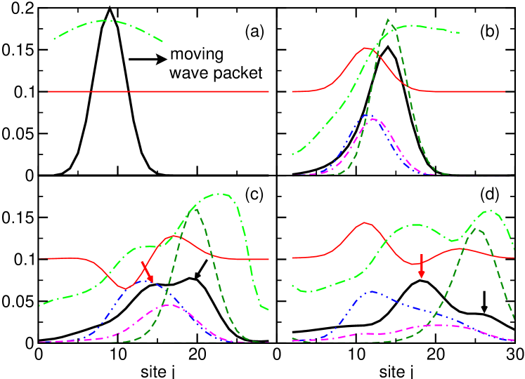
Figure 17: Snapshots of the polaron-formation process, for $t=\omega_{0}=1$, and $\bar{g}=0.4$. The calculation is performed on a 30-site periodic lattice. Time is measured in units of the phonon period. Shown are the electron density $\langle c_{j}^{\dagger}c_{j}\rangle$ (thick solid black line), phonon density $\langle b_{j}^{\dagger}b_{j}\rangle$ (blue double-dot dashed line), lattice displacement $\langle\hat{x}_{j}\rangle\equiv\langle b_{j}+b_{j}^{\dagger}\rangle$ (thin solid red line), velocity in units of lattice constant per phonon period (green dot dashed line), and EP correlation function $\langle c_{j}^{\dagger}c_{j}b_{j}^{\dagger}b_{j}\rangle$ (magenta dot double-dashed line). The green dashed line gives the free-electron wave packet for reference. For clarity, the origins of the thin solid red and green dashed curves are offset by 0.1 and their values are rescaled by a factor of 0.2 and $0.05/(2\pi)$ respectively. The blue double-dot dashed curve has been rescaled by a factor of 0.5.

There are regimes where the polaron formation time is a calculable constant of order unity times a phonon period $T_{0}$, as seen in some experiments and in Fig. 17, but there are other regimes in which the phonon period is not the relevant timescale. The limit of hopping $t\rightarrow 0$ is instructive KAK02 ; BLW86 . After a time $T_{0}/4$, the expectation of the lattice displacement $\langle\hat{x}_{j}\rangle$ on the electron site has the same value as a static polaron. It is tempting (but we would argue incorrect) to identify this as the polaron formation time. At later times, $\langle\hat{x}_{j}\rangle$ overshoots by a factor of two, and after a time $T_{0}$, $\langle\hat{x}_{j}\rangle$ and all other correlations are what they were at time zero when the bare electron was injected. The system oscillates forever. In general an electron emits phonons enroute to becoming a polaron, and we propose that the polaron formation time be defined as the time required for the polaron to physically separate from the radiated phonons. The polaron formation time for hopping $t\rightarrow 0$ is thus infinite, because the electron is forever stuck on the same site as the radiated phonons.

Figure 18: The on-site electron-phonon correlation function $\chi=\langle c_{j}^{\dagger}c_{j}(b_{j}+b^{\dagger}_{j})\rangle$ as a function of time measured in phonon periods. For all curves, $\omega_{0}=0.5$ and hopping $t=1$. The solid line is for a bare electron injected with nonzero initial momentum at energy $E_{i}=-0.7$, where the bottom of the bare band is at energy -2. The phonon displacement is larger and more weakly damped for larger electron-phonon coupling $\bar{g}$, dotted line. In contrast to a bare electron, an exciton (bound particle-hole pair) is generally created with an initial momentum zero, corresponding to $E_{i}=-2$, dashed line.

An electron injected at several times the phonon energy $\omega_{0}$ above the bottom of the band is another instructive example. The electron radiates successive phonons to reduce its kinetic energy to near the bottom of the band, and then forms a polaron. For very weak EP coupling, the rate for radiating the first phonon can be computed by Fermi’s golden rule, $\tau_{FGR}^{-1}=\bar{g}^{2}/[\hbar~{}t\sin(k_{f})],$ where $k_{f}$ is the electron momentum after emitting a phonon. The phonon emission time can be arbitrarily long for small $\bar{g}$. For strong coupling, the rate approaches $\tau_{SC}^{-1}=\bar{g}/\hbar$ because the polaron spectral function smoothly spans numerous narrow bands and its standard deviation is equal to $\bar{g}$.

Figure 19: Panel (a): Spectral function at strong coupling. There are three quasiparticle excited states split off from the continua. Shaded areas (1) and (2) correspond to continuum states. (b): Quantum beat formed by multiple excited states and continua.

Decaying oscillations in polaron formation (actually the formally equivalent problem of an exciton coupled to phonons Ra82 ) have been observed in a pump-probe experiment that measures reflectivity after a bare exciton is created SSKYK01 . The observed oscillatory reflectivity was interpreted as the lattice motion in the phonon-dressed (or “self-trapped”) exciton level. Assuming the modulation in the exciton level goes as $\Delta E=-\lambda c_{j}^{\dagger}c_{j}\hat{x}_{j}$, where $\hat{x}_{j}=\langle b_{j}+b^{\dagger}_{j}\rangle$ is the lattice displacement, the model Hamiltonian applies directly to the experiment. We calculate the corresponding EP correlation function in Fig. 18. In this regime, the polaron formation time (damping time) increases as the electron-phonon coupling $\bar{g}$ increases, and also as the initial electron (exciton) energy approaches the band bottom. We find satisfactory agreement when compared to Fig. 2b of Ref. SSKYK01 . Both show a damped oscillation with a delayed phase. (Numerical calculations in Figs. 18-19 are performed on an extended system, not a finite cluster.)

Figure 19 shows the spectral function at strong coupling. Three delta functions are visible, corresponding to polaron ground and excited states, along with three continua containing unbound phonons. There is additional structure at higher energy (not shown). The probability to remain in the initial bare particle state $P(\tau)\equiv|\langle\psi(\tau)|c_{k}^{\dagger}|0\rangle|^{2}$ for this spectrum is complicated, and includes oscillating terms that do not decay to zero at zero temperature from the polaron ground and excited states beating against each other. The branching ratios into the various channels are calculated in Ref. Ku03 .

6 Spectral signatures of Holstein polarons

As already stressed in the introduction the crossover from quasi-free electrons or large polarons to small polarons becomes manifest in the spectral properties above all. Here of particular interest is whether an “electronic” or “polaronic” (quasi-particle) excitation exists in the spectrum. This question has been partially addressed by calculating the wavefunction renormalisation factor [(electronic) quasi-particle weight] $Z_{k}$ in Sec. 3 (see Fig. 7). More detailed information can be obtained from the one-particle spectral function $A(k,\omega)$. This quantity of great importance can be probed by direct (inverse) photoemission, where a bare electron with momentum $k$ and energy $\omega$ is removed (added) from (to) the many-particle system. The intensities (transition amplitudes) of these processes are determined by the imaginary part of the retarded one-particle Green’s function, i.e. by

$$A(k,\omega)=-\frac{1}{\pi}{\rm Im}\,G(k,\omega)=A^{+}(k,\omega)+A^{-}(k,\omega)\,,$$ (30)

with

$$A^{\pm}(k,\omega) = -\frac{1}{\pi}{\rm Im}\!\!\lim_{\eta\to 0^{+}}\langle\psi_{0}|c_{k}^{\mp}\frac{1}{\omega+{\rm i}\eta\mp H}c_{k}^{\pm}|\psi_{0}\rangle$$ (31)

$$= \sum_{m}|\langle\psi_{m}^{\pm}|c_{k}^{\pm}|\psi_{0}\rangle|^{2}\delta[\,\omega\mp(E_{m}^{\pm}-E_{0})]\,,$$

where $c_{k}^{+}=c_{k}^{\dagger}$ and $c_{k}^{-}=c_{k}$ ($T=0$; 1D spinless case). These functions test both excitation energies ($E_{m}^{\pm}-E_{0}$) and overlap ($\propto Z_{k}$) of the $N_{e}$-particle ground state $|\psi_{0}\rangle$ with the exact eigenstates $|\psi_{m}^{\pm}\rangle$ of a $(N_{e}\pm 1)$–particle system. The electron spectral function of the single-particle Holstein model corresponds to $N_{e}=0$, i.e., $A^{-}(k,\omega)\equiv 0$. $A(k,\omega)$ can be determined, e.g., by a combination of KPM and CPT (cf. Sec. 2.2).

Figure 20 (a) shows that at weak EP coupling, the electronic spectrum is nearly unaffected for energies below the phonon emission threshold. Hence, for the case considered with $\omega_{0}$ lying inside the bare electron band $\varepsilon_{k}=-2t\cos k$, the signal corresponding to the renormalised dispersion $E_{k}$ nearly coincides with the tight-binding cosine band (shifted $\propto\varepsilon_{p}$) up to some $k_{X}$, where the phonon intersects the bare electron band. At $k_{X}$ electron and phonon states “hybridise” and repel each other, forming an avoided-crossing like gap. For $k>k_{X}$ the lowest absorption signature in each $k$ sector follows the dispersionless phonon mode, leading to the flattening effect WF97 . Accordingly the (electronic) spectral weight of these peaks is very low. The high-energy incoherent part of the spectrum is broadened $\propto\varepsilon_{p}$, with the $k$-dependent maximum again following the bare cosine dispersion.

Reaching the intermediate EP coupling (polaron crossover) regime a coherent band separates from the rest of the spectrum [$k_{X}\to\pi$; see panel (b)]. At the same time its spectral weight becomes smaller and will be transferred to the incoherent part, where several sub-bands emerge.

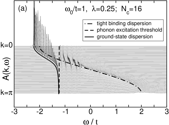
Figure 20: Spectral function of the 1D Holstein polaron in the weak (a), intermediate (b), and strong (c) EP coupling regimes. CPT data based on finite-cluster ED with $N_{c}$ sites, and $M=7$ ($\lambda=0.25$), $M=15$ ($\lambda=1$), $M=25$ ($\lambda=2$) phonon quanta. Note that the non-monotonic heights of the lowest energy peaks in (a) are an artifact of the CPT calculation, where some of the wavevectors fit the $N_{c}=16$ cluster size, and some don’t. Also the dispersionless absorption feature in (c), just above the small-polaron peak, is due to a finite-size effect, but not the double-peak structures of the higher excitation bands. This has been proved by determining the spectral function in the $k=0$–sector by VED.

The inverse photoemission spectrum in the strong-coupling case is shown in Fig. 20 (c). First, we observe all signatures of the famous polaronic band-collapse. The coherent quasi-particle absorption band becomes extremely narrow. Its bandwidth approaches the strong-coupling result $4Dt\exp(-g^{2})$ for $\lambda\,,g^{2}\gg 1$. If we had calculated the polaronic instead of the electronic spectral function, nearly all spectral weight would reside in the coherent part of the spectrum, i.e. in the small-polaron band. This has been demonstrated quite recently LHF06 . In our case the incoherent part of the spectrum carries most of the spectral weight. It basically consists of a sequence of sub-bands separated in energy by $\omega_{0}$, which correspond to excitations of an electron and one or more phonons.

Let us emphasise that for all couplings the lowest signature in $A(k,\omega)$ almost perfectly coincides with the coherent polaron band-structure (solid lines) obtained by VED (see Sec. 3), which underlines the high precision of the CPT-KPM approach used here.

Of course, the phonon modes are unaffected by one electron in the solid, i.e. the phonon self-energy is zero. Actually this is true in the thermodynamic limit only. In a finite-cluster calculation there will be an influence of order ${\cal O}(1/N)$ and the phonon spectra provide additional useful information concerning the polaron dynamics. For this purpose, we calculate the $T=0$ phonon spectral function

$$B(q,\omega)=-\frac{1}{\pi}{\rm Im}D^{R}(q,\omega)$$ (32)

which is related to the phonon Green’s function

$$D^{R}(q,\omega)=\lim_{\eta\to 0^{+}}\ \langle\psi_{0}|\hat{x}_{q}\frac{1}{\omega+{\rm i}\eta-H}\hat{x}_{-q}|\psi_{0}\rangle\,,$$ (33)

where $\hat{x}_{q}=N^{-1/2}\sum_{j}\hat{x}_{j}e^{-{\rm i}qj}$ and $\hat{x}_{j}=(b^{\dagger}_{j}+b_{j})/\sqrt{2\omega_{0}}$.

For the Holstein model (1), $B(q,\omega)$ is symmetric in $q$. The bare propagator $D_{0}(q,\omega)=2\omega_{0}/(\omega^{2}-\omega_{0}^{2})$ is dispersionless. Then, adapting the CPT-KPM approach to the calculation of the phonon spectral function, the cluster expansion is identical to replacing the full real-space Green’s function $D_{ij}$ by $D^{c}_{ij}$.

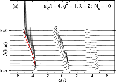
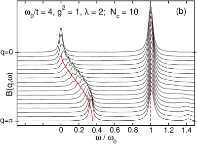
Figure 21: Electron (a) and phonon (b) spectral functions in the anti-adiabatic intermediate EP coupling regime. Solid (dashed) lines give $E_{k}$ ($\omega_{0}$) determined by VED. Note that abscissae are scaled differently.

Figure 21 compares electron (a) and phonon (b) spectra in the high phonon-frequency limit, where the small polaron crossover is determined by $g^{2}$. Obviously the phonon spectrum is also renormalised by the EP interaction due to the finite “particle density” $N_{e}/N_{c}=1/10$. So we can detect a clear signature of the polaron band having a width $W\simeq 1.5t$ (cf. Fig. 21 (a)). The dispersionless excitation at $\omega/\omega_{0}=1$ is obtained by adding one phonon with momentum $q$ to the $k=0$ ground state. Above this pronounced peak, we find an “image” of the lowest polaron band – shifted by $\omega_{0}$ – with extremely small spectral weight, hardly resolved in Fig. 21 (b).

7 Transport and optical response

The investigation of transport properties has been playing a central role in condensed matter physics for a long time. Optical measurements, for example, proved the importance of EP interaction in various novel materials such as the cuprates, nickelates or manganites and, in particular, corroborated polaronic scenarios for modelling their electronic transport properties at least at high temperatures Emi93 ; AM95 ; WMG98 . Actually, the optical absorption of small polarons is distinguished from that of large (or quasi-free) polarons by the shape and the temperature dependence of the absorption bands which arise from exciting the self-trapped carrier from or within the potential well that binds it Emi95 . Furthermore, as was the case with the properties of the ground state, the optical spectra of light and heavy electrons, small and large polarons differ significantly as well Ra82 . In the most simple weak-coupling and anti-adiabatic strong EP coupling limits, the absorption associated with photoionization of Holstein polarons is well understood and the optical conductivity can be analysed analytically (Emi93 ; Mah00 ; RH67 ; Lo88 ; Feea94 ; for a detailed discussion of small polaron transport phenomena we refer to Refs. Fi95 ; Fir ). The intermediate coupling and frequency regime, however, is as yet practically inaccessible for a rigorous analysis (here the case of infinite spatial dimensions, where dynamical mean-field theory yields reliable results, is an exception FC03 ; FC06 ). So far unbiased numerical studies of the optical absorption in the Holstein model were limited to very small 2 to 10-site 1D and 2D clusters AKR94 ; CSG97 ; FLW97 ; WF98a . In the following we will exploit the VED and KPM schemes EBKT03 ; SWWAF05 , in order to calculate the optical conductivity numerically in the whole parameter range on fairly large systems.

7.1 Optical conductivity at zero-temperature

Applying standard linear-response theory, the real part of the conductivity takes the form

$${\rm Re}\sigma(\omega)={\cal D}\delta(\omega)+\sigma^{reg}(\omega)\,,$$ (34)

where ${\cal D}$ denotes the so-called Drude weight at $\omega=0$ and $\sigma^{reg}$ is the regular part (finite-frequency response) for $\omega>0$ which can be written in spectral representation at $T=0$ as Mah00

$$\sigma^{reg}(\omega)=\frac{\pi}{\omega N}\sum_{E_{m}>E_{0}}|\langle\psi_{m}|\hat{\jmath}|\psi_{0}\rangle|^{2}\ \delta[\omega-(E_{m}-E_{0})]$$ (35)

with the (paramagnetic) current operator $\hat{\jmath}=-\mbox{i}et\sum_{i}(c_{i}^{\dagger}c_{i+1}-c_{i+1}^{\dagger}c_{i})$.

Introducing the $\omega$-integrated spectral weight,

$$S^{reg}(\omega)=\int_{0^{+}}^{\omega}\,d\omega^{\prime}\sigma^{reg}(\omega^{\prime})\,,$$ (36)

we arrive at the f-sum rule

$$-E_{kin}/2={\cal D}+S^{reg}/\pi\qquad{\rm(1D\;case)}\,,$$ (37)

where $E_{kin}=-t\sum_{i}(c_{i}^{\dagger}c_{i+1}+c_{i+1}^{\dagger}c_{i})$ is the kinetic energy and $S^{reg}=S^{reg}(\infty)$. Since for the Holstein model the Drude weight can be calculated independently from Kohn’s formula or the effective mass,

$${\cal D}=\frac{1}{2N}\frac{\partial^{2}E_{0}(\Phi)}{\partial\Phi^{2}}\Big{|}_{\Phi=0}=\frac{1}{2N}\frac{\partial^{2}E_{k}}{\partial k^{2}}\Big{|}_{k=0}=\frac{1}{2m^{*}}\,,$$ (38)

the f-sum rule may be used to test the numerics. In Eq. (38), the first equality relates ${\cal D}$ to the second derivative of the (non-degenerate) ground-state energy with respect to a field-induced phase $\Phi$ coupled to the hopping.

We first present $\sigma^{reg}(\omega)$ and its integral $S^{reg}(\omega)$ for the 1D Holstein model in Fig. 22. The upper panel (a) gives the results for intermediate-to-strong EP coupling, i.e. near the polaron crossover, in the adiabatic (light electron) regime. Of course, the optical conductivity threshold is $\omega=\omega_{0}$ for the infinite system we deal with using VED. In this respect standard ED, defined on finite lattices, suffers from pronounced finite-size effects due to the discreteness in $k$-space. Knowing that at about $\lambda\simeq 1$ a coherent polaron band with bandwidth much smaller than $\omega_{0}$ splits off, the first (few) isolated peak(s) at the lower bound of the spectrum can be attributed to one- (few-) ($q=0-$) phonon emission processes (cf. also Fig. 20 (b)). Of course, these transitions have little spectral intensity. At higher energies transitions to the incoherent part of the spectrum take place by “emitting” phonons with finite momentum (to reach the total momentum $k=0$ ground-state sector). The main signature of $\sigma^{reg}(\omega)$ is that the spectrum is strongly asymmetric, which is characteristic for rather large polarons. The weaker decay at the high-energy side meets the experimental findings for many polaronic materials like ${\rm TiO_{2}}$ KMF69 even better than standard small-polaron theory.

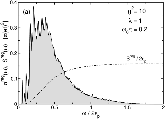
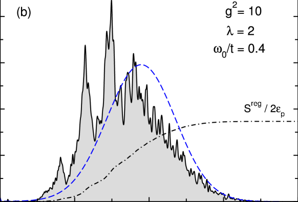
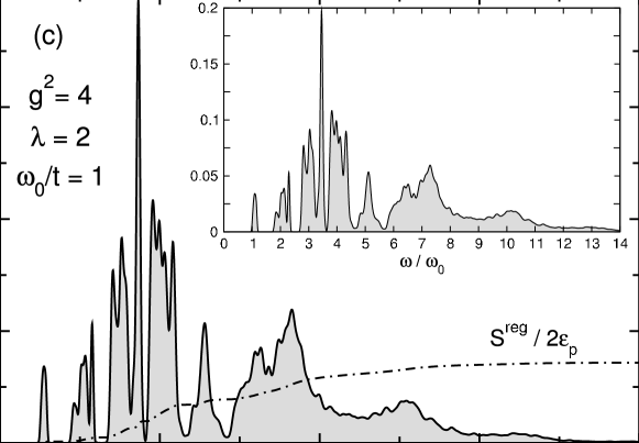
Figure 22: Optical conductivity of the 1D Holstein polaron at $T=0$. Results for $\sigma^{reg}(\omega)$ and $S^{reg}(\omega)$ are obtained by VED. In order to reduce finite-$M$ effects, data calculated for $M=15$ to 20 were averaged. The dashed line in (b) displays the analytical small polaron result, $\sigma^{reg}(\omega)=\frac{\sigma_{0}}{\sqrt{\varepsilon_{p}\omega_{0}}}\frac{1}{\omega}\exp\left[-\frac{(\omega-2\varepsilon_{p})^{2}}{4\varepsilon_{p}\omega_{0}}\right]$ (cf. Ref. Emi93 ), where $\sigma_{0}$ was determined to give the same integrated spectral weight as $\sigma^{reg}(\omega>0)$.

For $\lambda=2$ and $\omega_{0}=0.4$, i.e., at larger EP coupling, but not yet in the small-polaron limit, we find a more pronounced and symmetric maximum in the low-temperature optical response (see Fig. 22 (b)). The maximum is located below the corresponding one for small polarons at $T=0$, which on its part lies somewhat below $2\varepsilon_{p}=2t\lambda=2g^{2}\omega_{0}$ (being the maximum of the Poisson distribution) because of the $1/\omega$ factor contained in the conductivity. In this case the polaron band structure is more strongly renormalised, but, more importantly, the phonon distribution function in the ground state becomes considerably broadened. Since the current operator connects only different-parity states having substantial overlap as far as the phononic part is concerned, in the optical response multi-phonon emissions/absorptions (i.e., non-diagonal transitions Mah00 ) become increasingly important. Again deviations from the analytical small-polaron result (dashed line in Fig. 22 (b)) might be important for relating theory to experiment.

The optical response obtained if the phonon frequency becomes comparable to the electron transfer amplitude is illustrated in Fig. 22 (c). Now the lowest one-phonon absorption (threshold) signal is well separated. In contrast to the light electron case Fig. 22 (a), the different absorption bands appearing for a heavier electron can be classified according to the number of phonons involved in the optical transition (see inset). Increasing $\omega_{0}$ at fixed $g^{2}$ this becomes even more manifest (at the same time a Poisson distribution of the different sub-bands evolves). The sub-bands are broadened by transitions to different “electronic” levels. For our parameters, a scattering continuum appears above $\omega>5$ to $6~{}\omega_{0}$. Note that the “fragmentation” of the spectrum appearing at smaller energy transfer is not caused by finite-size effects.

Turning to the sum rules presented in Fig 23, we notice a monotonic decrease of the total sum rule $S^{tot}/\pi=-E_{kin}/2$, which indicates a suppression of the electronic kinetic energy with increasing EP coupling. In agreement with previous numerical results RL82 ; WF98a ; HEL04 , the kinetic energy clearly shows the crossover from a large polaron, characterised by a $E_{kin}$ that is only weakly reduced from its non-interacting value [$E_{kin}(\lambda=0)=-2t$], to a less mobile small polaron in the strong EP-coupling limit, where the strong-coupling perturbation theory result,

$$E_{kin}^{SCPT}=-\frac{4t}{\omega_{0}}\Big{\langle}\frac{1}{s}\Big{\rangle}_{\kappa=2g^{2}}-\mbox{e}^{-g^{2}}\left[2+\frac{4t}{\omega_{0}}\Big{\langle}\frac{1}{s}\Big{\rangle}_{\kappa=g^{2}}\right]$$ (39)

($\langle\ldots\rangle_{\kappa}$ denotes the average with respect to the Poisson distribution with parameter $\kappa$), gives a sufficiently accurate description in both the adiabatic and antiadiabatic regimes.

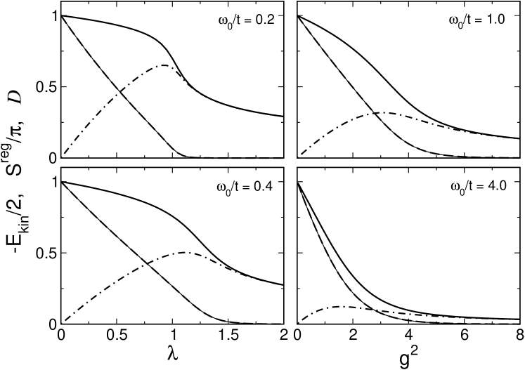
Figure 23: Renormalised kinetic energy ($E_{kin}$; solid line) and contribution of $\sigma^{reg}$ to the f-sum rule ($S^{reg}$; dot-dashed line) as a function of the EP couplings $\lambda$ and $g$ in the adiabatic (left panels) and non-to-antiadiabatic (right panels) regimes, respectively. The Drude weights were obtained from the f-sum rule [(Eq. (37); thin solid line)] and effective mass [(Eq. (38); dashed line)].

For light electrons (adiabatic regime $\omega_{0}/t=0.2,\;0.4$; left panels), we found a rather narrow transition region. The drop of $S^{tot}$ in the crossover region $\lambda\simeq 1$ is driven by the sharp fall of the Drude weight, which is a measure of the coherent transport properties of a polaron. By contrast the optical absorption due to inelastic scattering processes, described by the regular (dissipative) part of the optical conductivity, becomes strongly enhanced around $\lambda\simeq 1$ FLW97 (cf. the behaviour of $S^{reg}$).

The large to small polaron crossover is considerably broadened for heavy electrons (non-to-antiadiabatic case $\omega_{0}/t=1,\;4$; right panels). Here $E_{kin}$ decreases more gradually and $S^{reg}$ exhibits a less pronounced maximum at about $g^{2}=1$.

As quoted above, we can calculate the Drude weight independently from the effective mass of the Holstein polaron. Using this data, it is worth mentioning that the f-sum rule (37) is satisfied numerically to at least six digits in the whole parameter regime EBKT03 .

7.2 Thermally activated transport

If the polaron effects are assumed to be dominant the coherent bandwidth is extremely small. Then the physical picture is that the particle is trapped at a certain lattice site and that hopping occurs infrequently from site to site. There are two kinds of transfer processes Ho59b . All phonon numbers might remain the same during the hop (diagonal transition) or, alternatively, the number of phonons is changed (non-diagonal transition). In the latter case each hop may be approximated as a statistically independent event and the particle loses its phase coherence by this phonon emission or absorption (inelastic scattering). Diagonal and non-diagonal transitions show a different temperature dependence. While the rate of diagonal (band-type) transitions decreases with increasing temperature, small-polaron theory predicts that the non-diagonal (incoherent hopping) rate is thermally activated and may become the main transport process at higher temperatures (cf., e.g., Ref. Mah00 ). Deviations from standard small-polaron theory are expected to occur in the intermediate coupling regime. By means of ED and KPM techniques we are able to study the optical response of Holstein polarons precisely in this regime, at least for small lattices.

ac conductivity

Our starting point is the Kubo formula for the electrical conductivity at finite temperatures Mah00 ,

$$\sigma^{reg}(\omega;T)=\frac{\pi}{\omega N}\frac{1}{Z}\sum_{m,n>0}^{\infty}\left[{\rm e}^{-\beta E_{n}}-{\rm e}^{-\beta E_{m}}\right]\,|\langle\psi_{n}|\hat{\jmath}|\psi_{m}\rangle|^{2}\,\delta(\omega-\omega_{mn})\,,$$ (40)

where $Z=\sum_{n}^{\infty}\mathrm{e}^{-\beta E_{n}}$ is the partition function and $\beta=T^{-1}$ denotes the inverse temperature ($k_{B}=1$). Since in practice the contribution of highly excited phonon states is negligible at the temperatures of relevance, the system is well approximated by a truncated phonon space with at most $M(\lambda,g,\omega_{0};T)$ phonons BWF98 . Then $|\psi_{n}\rangle$ and $|\psi_{m}\rangle$ are the eigenstates of $H$ within our truncated Hilbert space. $E_{n}$ and $E_{m}$ are the corresponding eigenvalues with $\omega_{mn}=E_{m}-E_{n}$.

In order to evaluate temperature-dependent response functions like (40), recently a generalised “two-dimensional” KPM scheme has been proposed WWAF06 ; SWWAF05 , which, in our case, can be set up using a current operator density

$$j(x,y)=\sum_{m,n}|\langle\psi_{n}|\hat{\jmath}|\psi_{m}\rangle|^{2}\ \delta(x-E_{n})\ \delta(y-E_{m})\,.$$ (41)

For the regular part of the conductivity we obtain

$$\sigma^{reg}(\omega)=\frac{2\pi}{\omega N}\frac{1}{Z}\int\limits_{0^{+}}^{\infty}j(y+\omega,y)\big{[}{\rm e}^{-\beta y}-{\rm e}^{-\beta(y+\omega)}\big{]}\,dy\,,$$ (42)

where the partition function $Z=2\int_{0^{+}}^{\infty}\rho(E)\exp(-\beta E)$ is easily obtained by integrating over the density of states $\rho(E)=\sum_{n=0}^{D-1}\delta(E-E_{n})$, which can be expanded in parallel to $j(x,y)$ (here $D$ is the dimension of the Hilbert space). One advantage of this approach is that the current operator density that enters the conductivity is the same for all temperatures, i.e., it needs to be expanded only once.

Figure 24 gives results for the finite-temperature optical conductivity of a Holstein polaron. Coherent transport related to diagonal transitions within the lowest polaron band is negligible at high temperatures. For instance, the amplitude of the current matrix elements between the degenerate states with momentum $K=\pm\pi/3$ ($K=0,\,\pm\pi/3,\,\pm 2\pi/3$, and $\pi$ are the allowed wave numbers of our 6-site system with periodic boundary conditions) is of the order of $10^{-7}$ only. In the small polaron limit , where the polaronic sub-bands are roughly separated by the bare phonon frequency, non-diagonal transitions become important for $T>\omega_{0}$. Let us consider the activated regime in more detail (see Fig. 24 (upper panel)). With increasing temperatures we observe a substantial spectral weight transfer to lower frequencies, and an increase of the zero-energy transition probability in accordance with previous results Na63 .

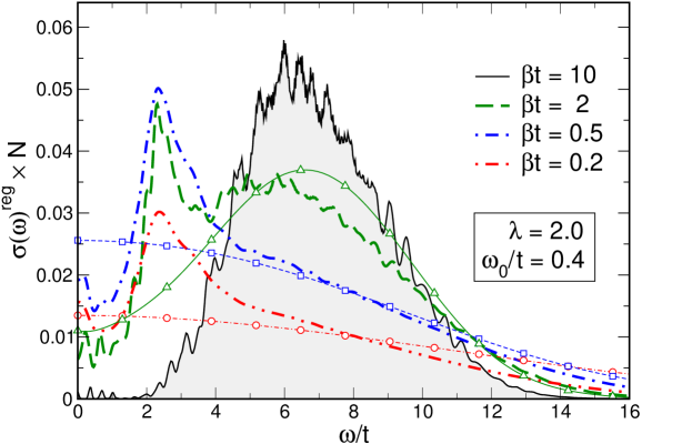
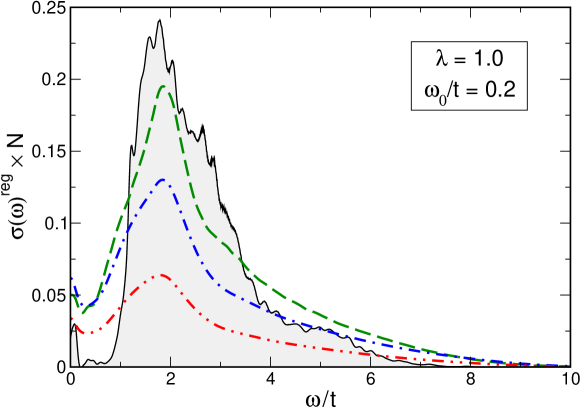
Figure 24: Optical absorption by Holstein polarons at finite temperatures in the adiabatic strong (upper panel) and intermediate (lower panel) EP coupling regime. Results are obtained by ED for a $N=6$ site lattice with $M=45$ phonons. In the upper panel, thin lines with symbols give the analytical results for the small polaron transport BB85 ; Mah00 at temperatures $\beta t=2$ (triangles), $0.5$ (squares), $0.2$ (circles). The deviations observed for high excitation energies at very large temperatures are caused by the necessary truncation of the phonon Hilbert space in ED.

In addition, we find a strong resonance in the absorption spectra at about $\omega_{0}\sim 2t$, which can be easily understood using a configurational coordinate picture SWWAF05 . In order to activate these transitions thermally, the electron has to overcome the “adiabatic” barrier $\Delta=E_{1+}-E_{0}=\varepsilon_{p}/2-t$, where we have assumed that the first relevant excitation is a state with lattice distortion spread over two neighbouring sites and the particle mainly located at both these sites (in a symmetric ($+$) or antisymmetric ($-$) linear combination; $E_{1,\pm}=\mp t-\varepsilon_{p}/2$). A finite phonon frequency will relax this condition. From Fig. 24, we find the signature to occur above $T>0.5t$. Obviously this feature is absent in the standard small-polaron transport description which essentially treats the polaron as a quasiparticle without resolving its internal structure.

Now let us decrease the EP coupling strength $\lambda$ keeping $g^{2}=10$ fixed. Results for the optical response in the vicinity of the large to small polaron crossover are depicted in the lower panel of Fig. 24. Here the small polaron maximum has almost disappeared and the $2t$-absorption feature can be activated at very low temperatures ($\Delta\to 0$ for the two-site model with $\lambda=1$). The gap observed at low frequencies and temperatures is clearly a finite-size effect. The overall behaviour of $\sigma^{reg}(\omega;T)$ resembles that of polarons of intermediate size. At high temperatures these polarons will dissociate readily and the transport properties are equivalent to those of electrons scattered by thermal phonons. Let us emphasise that many-polaron effects become increasingly important in the large-to-small polaron transition region Hoea05 (see also Sec. 8 below). As a result, polaron transport might be changed entirely compared to the one-particle picture discussed so far.

dc conductivity and thermopower

We consider dc transport, or $\sigma(\omega)$ in the limit $\omega\rightarrow 0$. For simplicity, we consider only a single polaron, or a dilute system of polarons where interactions can be neglected and bipolaron formation is prevented, as by a large repulsive $U$. We also neglect impurities, which can localise or scatter a polaron.

At zero temperature, the conductivity or mobility of a polaron is infinite. The polaron can be placed in a state of nonzero momentum by a weak electric field acting for a short time. This is an eigenstate, which carries current forever and never decays. At small temperatures $T\ll\omega_{0}$, an exponentially small number of phonons are thermally excited. The conductivity becomes finite due to scattering of a polaron off thermally excited phonons of density $n_{ph}\sim e^{-\omega_{0}/T}$. The details depend on the EP scattering process.

In 1D, when a polaron of momentum $k$ encounters a thermally excited phonon, in general part of it is transmitted and part is backscattered. Certain anomalies occur. For example, in the limit of small hopping $t$, as $g$ approaches 1, the backscattering of the polaron vanishes and the phonon is simultaneously transferred one site in the direction opposite the polaron momentum. The phonon thus recoils opposite to the direction expected, cf. the collision of two balls. This leads to a heat current in the opposite direction as the polaron particle current, which should be observable in the thermopower. A polaron-thermal phonon bound state also exists for sufficiently large $g$. For this bound state, heat (a phonon excitation) can be transported by an electric field, which again should be observable as a large contribution to the thermopower of the opposite sign as the above. For large $g$, this bound state or internal polaron excited state can have a much smaller effective mass than the polaron ground state. Perhaps surprisingly, as the temperature increases, the polaron effective mass as measured by the low-frequency ac conductivity can decrease.

We next consider very high temperatures. As $T$ increases, the typical phonon displacement increases as $\tilde{K}\langle\hat{x}^{2}\rangle=k_{B}T$, where $\tilde{K}$ is the phonon spring constant. For quasi-static phonons (large phonon mass), this leads to a disorder potential for the electron that increases without bound as $T$ increases. The disorder Anderson localises the electron, leading to zero dc conductivity. The disorder, however, is not quite static, and rearranges itself on a timescale $\tau\sim 1/\omega_{0}$. Once every time of order $\tau$, the diagonal energies of the electron site and a neighbouring site become equal, and the electron can hop to a neighbouring site. It is then diffusing with a diffusion constant $\sim a^{2}\omega_{0}$, where $a$ is the lattice constant. Using the Einstein relation relating diffusion and mobility, the high temperature resistivity becomes

$$\rho={\pi k_{B}T\over ne^{2}a^{2}\omega_{0}}.$$ (43)

The high temperature resistivity is metallic, i.e. $d\rho/dT>0$, and can greatly exceed the Ioffe-Regel limit. Numerical studies to confirm or refute this scenario are incomplete.

8 From few to many polarons

Let us now address the important issue of how the character of the (polaronic) quasiparticles may change if we increase the carrier density $n=N_{e}/N$. Consider first the case of zero electron-electron interaction. Beginning with a noninteracting Fermi gas at $T=0$, as the Holstein EP interaction $g$ is increased from zero, a singlet superconductor is expected to form. As $g$ increases, the diameter of the Cooper pair decreases. Eventually, the Cooper pair diameter becomes smaller than the distance between Cooper pairs, and the behaviour crosses over from BCS superconductivity to that of Bose condensation, like that of ⁴He, where the hard core bosons are bipolarons (bound states of two polarons). In this limit, $T_{c}$ is given approximately by the Bose condensation temperature for ideal bosons of mass $m^{*}$, where $m^{*}$ is the bipolaron mass. The limit of Bose condensation of bipolarons is not given correctly by Eliashberg theory, which describes strong coupling, but not that strong.

8.1 Bipolaron formation

We investigate how two electrons coupled to phonons may bind together to form a bipolaron, including the bipolaron effective mass, the crossover between two different types of bound states, and the dissociation into two polarons (see also Ale ; Aub ). For problems with more than one electron, the Holstein Hamiltonian is generalised by adding a Hubbard electron-electron interaction term, $U\sum_{j}n_{j\uparrow}n_{j\downarrow}$. Basis states for the many-body Hilbert space can be written $|b\rangle=|j_{1},j_{2};\dots,n_{m},n_{m+1},\dots,\rangle$, where the up and down electrons are on sites $j_{1}$ and $j_{2}$, and there are $n_{m}$ phonons on site $m$. In a generalisation of the one electron VED method described above, a bipolaron variational space is constructed beginning with an initial state where both electrons are on the same site with no phonons, and operating repeatedly ($L$-times) with the off-diagonal pieces ($t$ and $\bar{g}$) of the Hamiltonian. All translations of these states are included on an infinite lattice. The method is very efficient in the intermediate coupling regime, where it provides results that are variational in the thermodynamic limit and bipolaron energies that are accurate to 7 digits for the case $L=18$ and size of the Hilbert space $N_{st}=2.2\times 10^{6}$ phonon and down electron configurations for a given up electron position. In 1D the size of the variational space approximately doubles as $L$ is increased by one, which is the same as for the one electron problem, although the prefactor for two electrons is larger BKT00 .

For large phonon frequency $\omega_{0}$, the EP interaction leads to a non-retarded attractive on-site interaction of strength $U_{0}\equiv 2\omega_{0}g^{2}$. One would expect that as the Hubbard repulsion $U$ becomes larger than this value, the bipolaron would dissociate into two polarons. As can be shown both analytically and numerically, this is not what happens. In the limit of small hopping $t$, as $U$ exceeds $U_{0}$, the bipolaron crosses over from a state S0 with both electrons primarily on the same site, to another bound state S1 with the electrons primarily on nearest neighbour sites. Only for $U>2U_{0}$ does the bipolaron dissociate into two polarons. The crossover from $S0$ to $S1$ bipolarons is important in theories of bipolaronic superconductivity applied to real materials, since S1 bipolarons are generally orders of magnitude lighter than S0 bipolarons. Since the superconducting $T_{c}$ in the dilute limit is inversely proportional to the effective mass, the S1 regime usually provides a more compelling theory.

We now discuss numerical variational results for the singlet bipolaron on an infinite 1D lattice. We have been unable to demonstrate the existence of a bound triplet bipolaron for the Holstein-Hubbard model. Fig. 25 shows the ground state electron-electron density correlation function $C(i-j)=\langle\psi_{0}|n_{i}n_{j}|\psi_{0}\rangle$, where $n_{i}=n_{i\uparrow}+n_{i\downarrow}$ and $|\psi_{0}\rangle$ denotes the ground state wave function. At $g=1$, the bipolaron widens with increasing $U$ and transforms into two unbound polarons (which can only move a finite distance apart in the variational space). The value $U=1.5$ is below the transition to the unbound state at $U_{c}=2.17$, calculated by comparing the polaron and bipolaron energies. We see that the probability of electrons occupying the same or neighbouring sites is almost equal. In the unbound regime, the nature of the correlation function changes significantly. At $U=1.5$, $C(i)$ falls off exponentially, while for $U>U_{c}$ the typical distance between electrons is the order of the maximum allowed separation $L$. The electrons can be no farther apart than $L$ in the variational space, although their centre of mass can be anywhere on an infinite lattice. A state of separated polarons is clearly seen for $U=20$.

Two distinct regimes are seen at $g=2$ within the bipolaronic region. At $U=7<U_{0}\equiv 2\omega_{0}g^{2}=8$, the correlation function represents the S0 bipolaron, while at $U=9>U_{0}$ we find the largest probability for two electrons to be on neighbouring sites, which is characteristic of the S1 bipolaron. In contrast to previous calculations where phonons were treated classically PA98 , we find a crossover rather than a phase transition between the two regimes. Moving from strong towards intermediate coupling, the S0 and S1 bipolarons consist of longer exponential tails extending over many lattice sites, and the two regimes can no longer be distinguished. The precision of presented correlation functions in the bipolaron regime is within the size of the plot symbols in the thermodynamic limit.

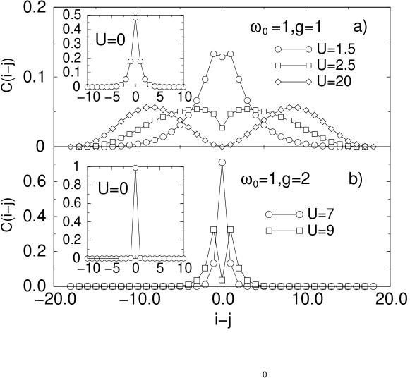
Figure 25: Electron-electron correlation function $C(i-j)$ calculated at $\omega_{0}=1$, a) $g=1$ and b) $g=2$ for different values of $U$, with $L=18$. The two ordinate axes have a different range. Insets show results for $U=0$. All curves are normalised, $\sum_{i}C(i)=1$.

Figure 26a plots the bipolaron mass ratio $R_{m}=m_{bi}/2m_{po}$ vs. $U$ for different values of $\omega_{0}$ and $g$. In all cases presented in Fig. 26, $R_{m}$ approaches 1 as $U$ approaches $U=U_{c}$ in agreement with a state of two free polarons. At fixed $\omega_{0}=1$ the bipolaron mass ratio increases by several orders of magnitude with increasing $g$ at $U=0$. Increasing $U$ sharply decreases $R_{m}$ in the S0 regime. Note that the mass scale is logarithmic. In the S1 regime with $U>U_{0}$, $R_{m}$ is small, as predicted by the strong coupling result.

Figure 26: a) The mass ratio $R_{m}=m_{bi}/2m_{po}$ vs. $U$ and b) the bipolaron isotope effect $\alpha_{I}$ vs. $U$. Numerical results are for $L=18$. Results for $R_{m}$ at $\omega_{0}=0.5$ are obtained by extrapolating $L\to\infty$. Precision in all curves is within the line-width in the thermodynamic limit, except for $\alpha_{I}$ with $\omega_{0}=0.5$, where the error is estimated to be $\pm 5\%$. The thin line in (a) is the strong coupling expansion result for $\omega_{0}=1$, $g=2$. Polaron masses in units of the noninteracting electron mass are $m_{po}=1.35,1.76,10.4,3.06$ from top to bottom respectively.

In the dilute bipolaron regime, the bipolaron isotope effect is the same as the classic superconductivity isotope effect for $T_{c}$. The bipolaron isotope effect, shown in Fig. 26b, is large in the strong coupling ($\omega_{0}=1,g=2$) and small $U$ regime, where its value is somewhat below the large $g$ strong coupling prediction $\alpha_{I,S0}\sim 2g^{2}-{1\over 4}=7.75$. With increasing $U$, $\alpha_{I}$ decreases and in the S1 regime approaches $\alpha_{I,S1}=g^{2}/2=2$. A kink is observed in the crossover regime. With decreasing $g$ or $\omega_{0}$, $\alpha_{I}$ also decreases.

The phase diagram $U_{c}(g)$ is shown in Fig. 27 at fixed $\omega_{0}=1$. Numerical results, shown as circles, indicate the phase boundary between two dissociated polarons each having energy $E_{po}$ and a bipolaron bound state with energy $E_{bi}$. In the inset of Fig. 27 we show the bipolaron binding energy defined as $\Delta=E_{bi}-2E_{po}$. The phase diagram is obtained from $\Delta=0$. The dashed line, given by $U_{0}=2\omega_{0}g^{2}$, is a reasonable estimate for the phase boundary at small $g$. At large $g$ the dashed line roughly represents the crossover between a massive S0 and lighter S1 bipolaron. The S1 region grows with increasing $g$. The dot-dashed line is the phase boundary between S1 and the unbound polaron phase, as obtained by degenerate strong coupling perturbation theory. Numerical results approach this line at larger $g$. The dot-dashed line asymptotically approaches $U_{c}=4\omega_{0}g^{2}$.

Figure 27: Phase diagram and binding energy $\Delta$ in units of $t$ (inset) calculated at $\omega_{0}=1$. Numerical results are circles. For greater accuracy, results near the weak and strong coupling regime were obtained by extrapolating $L\rightarrow\infty$.

8.2 Many-polaron problem

We consider how polarons evolve from the dilute to the concentrated limit, in the regime where spinless or fully spin-polarised fermions prevent bipolaron formation. In 1D with open boundary conditions, the spinless fermion problem is equivalent to infinite Hubbard $U$. While for very strong EP coupling no significant changes are expected due to the existence of rather independent small (self-trapped) polarons with negligible residual interaction (assuming spinless fermions or strong enough electron-electron repulsion to prevent bipolaron formation), a density-driven crossover from a state with large polarons to a metal with weakly dressed electrons should occur in the intermediate-coupling regime. This issue has recently been investigated theoretically by ED CGS99 , QMC Hoea05 , and variational canonical transformation LHF06 methods, and is known to be of experimental relevance, e.g., in ${\rm La_{2/3}(Sr/Ca)_{1/3}MnO_{3}}$ films HMDLK04 .

In the spinless fermion Holstein model, the above-mentioned density-driven transition from large polarons to weakly EP-dressed electrons is expected to be possible only in 1D, where large polarons exist at intermediate coupling. The situation is different for Fröhlich-type models Fr54 ; AK99 ; DT01 with long-range EP interaction, in which large-polaron states exist even for strong coupling and in $D>1$.

To set the stage, we first comment on the evolution of the one-electron spectral function $A(k,\omega)$ with increasing electron density $n$ in the weak- and strong-coupling limiting cases Hoea05 . In the former the spectra bear a close resemblance to the free-electron case for all $n$, i.e., there is a strongly dispersive band running from $-2t$ to $2t$, which can be attributed to weakly dressed electrons with an effective mass close to the non-interacting value. As expected, the height (width) of the peaks increases (decreases) significantly in the vicinity of the Fermi momentum. In the opposite strong-coupling limit the spectrum exhibits an almost dispersionless coherent polaron band $\forall\;n<0.5$. Besides, there are two incoherent features located above and below the Fermi energy, broadened $\propto\varepsilon_{p}$, which are due to phonon-mediated transitions to high-energy electron states. The most important point, however, is the clear separation of the coherent band from the incoherent parts even at large $n$, indicating that small polarons are well-defined quasiparticles in the strong-coupling regime, even at high carrier density.

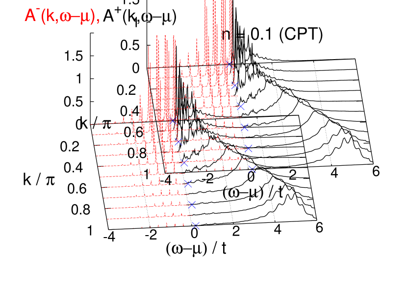
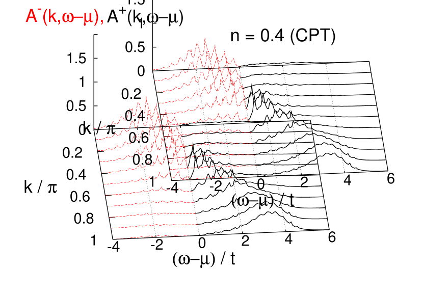
Figure 28: Single particle spectral functions $A^{-}(k,\omega)$ (red dashed lines) and $A^{+}(k,\omega)$ (black solid lines) for two characteristic band fillings, $n=0.1$ and $n=0.4$, at $\omega_{0}/t=0.4$ and $\lambda=1$ ($T=0$). Results are obtained by CPT using $N_{c}=10$). Blue crosses track the small-polaron band determined by ED.

Figure 28 displays the inverse photoemission [$A^{+}(k,\omega)$] and photoemission spectra [$A^{-}(k,\omega)$] at intermediate EP coupling strength, determined by CPT. At low densities, $n=0.1$ (upper panel), we can easily identify a (coherent) polaron band crossing the Fermi energy level $E_{F}=\mu(T\to 0)$, the latter being situated at the point where $A^{-}$ and $A^{+}$ intersect. This large-polaron band has rather small electronic spectral weight especially away from $E_{F}$ and flattens at large $k$, as known from single-polaron studies (see Sec. 6, Fig. 20). Below this band, there exist equally spaced phonon satellites, reflecting the Poisson distribution of phonons in the ground state. Above $E_{F}$ there is a broad dispersive incoherent feature whose maximum closely follows the dispersion relation of free particles.

As the density $n$ increases, a well-separated coherent polaron band can no longer be identified. At about $n\simeq 0.3$ the deformation clouds of the (large) polarons start to overlap leading to a mutual (dynamical) interaction between the particles. Increasing the carrier density further, the polaronic quasiparticles dissociate, stripping their phonon cloud. This is the case shown in the lower panel of Fig. 28. Now diffusive scattering of electrons and phonons seems to be the dominant interaction mechanism. As a result both the phonon peaks in $A^{-}(k,\omega)$ and the incoherent part of $A^{+}(k,\omega)$ are washed out, the spectra broaden and ultimately merge into a single wide band. Most notably, the incoherent excitations now lie arbitrarily close to the Fermi level. Obviously the low-energy physics of the system can no longer be described by single-particle small-polaron theory.

9 Polaronic effects in strongly correlated systems

The interplay of electron-electron and electron-phonon interactions in the formation of dressed quasiparticles is becoming the focus of attention in many contexts, including conducting polymers, ferroelectrics, halide-bridged transition-metal chain complexes, and several important classes of perovskites. Especially research on high-${\rm T_{c}}$ superconductivity (HTSC) and colossal magnetoresistance (CMR) has spurred intense investigations of the competition or, if possible, of the cooperation of these two fundamental interactions (for a recent review see Eg06 , and references therein).

Many experiments have indicated substantial EP interaction in the high-${\rm T_{c}}$ cuprates. The relevance of EP coupling can be seen from the experimental observation of phonon renormalisation Ri94 . Ion channelling SRBL89 ; Hagea90 , neutron scattering Egea91 and photo-induced absorption measurements Kiea88 proved the existence of large anharmonic lattice fluctuations, which may be responsible for local phonon-driven charge instabilities in the planar $\rm CuO_{2}$ electron system Jo91 ; ZS92 . Photo-induced absorption experiments MFVH90 , infrared spectroscopy Caea94 and reflectivity measurements FLKB93 indicate the formation of small polarons in the insulating parent compounds $\rm La_{2}CuO_{4+y}$ and $\rm Nd_{2}CuO_{4-y}$ of the hole- and electron-doped superconductors $\rm La_{2-x}Sr_{x}CuO_{4+y}$ and $\rm Nd_{2-x}Ce_{x}CuO_{4-y}$, respectively. Recently angle-resolved photoemission spectroscopy data were interpreted in terms of strong EP coupling giving rise to self-localisation of holes (hole polarons) Roea05 . Based on these experimental findings, several theoretical groups VPD91 ; Emi92b ; Emi94 ; AK92 ; AR92b ; ABMS93 ; Hi93 ; Mot93 ; AM94 ; Ra94 ; ICNC95 promote a (bi)polaronic scenario for HTSC.

Even stronger evidence for polaron formation in doped charge transfer oxides is provided by experiments on the nickelates $\rm La_{2-x}Sr_{x}NiO_{4}$ BE93 ; CCC93 . The isostructural compounds $\rm La_{2}CuO_{4}$ and $\rm La_{2}NiO_{4}$ show a remarkable difference upon the substitution of La by Sr. Both materials become metallic upon doping, but in the nickelates a nearly total substitution of La for Sr is necessary. Also in $\rm La_{2-x}Sr_{x}NiO_{4+y}$ no superconductivity is found for any $x$. A resolution of this problem might be given by extended LDA calculations AKZA92 , which show that the nickelates are much more susceptible to a breathing polaron instability than the cuprates. The reason is the much stronger magnetic confinement effect of additional holes and nickel spins. These low–spin composite holes are nearly entirely prelocalised and the EP coupling becomes much more effective in forming polarons. For the composition $\rm La_{1.5}Sr_{0.5}NiO_{4}$ (quarter filling, $x=0.5$), electron diffraction measurements show a commensurate superstructure spot at the $(\pi,\pi)$-point, which has been interpreted as a sign of truly 2D ordering of breathing-type polarons, i.e., as a polaronic superlattice.

Localised lattice distortions are also suggested to play an important role in determining the electronic and magnetic properties of hole-doped manganese oxides of the form $\rm La_{1-x}[Sr,Ca]_{x}MnO_{3}$ ZCKM96 ; Mi98 . In the region $x_{MI}\sim 0.2<x<0.5$ these compounds show a transition from a metallic ferromagnetic low-temperature phase to an insulating paramagnetic high-temperature phase associated with a spectacularly large negative magnetoresistive response to an applied magnetic field JTMFRC94 . Both breathing-mode collapsed ($\rm Mn^{4+}$) and (anti) Jahn-Teller distorted ($\rm Mn^{3+}$) sites are created simultaneously when the holes are localised in passing the metal-insulator transition AP99 ; BPPSK00 . The relevance of small polaron transport above $T_{c}$ is obvious from the activated behaviour of the conductivity WMG98 . Consequently many theoretical studies focused on polaronic approaches AB99 ; Caea97 ; LM97 ; Quea98 ; KJN98 ; Mu99 ; Deea99 ; WLF03 . Polaronic features have been established by a variety of experiments. For example, high-temperature thermopower JSRTHC96 ; PRCZSZ97 and Hall mobility measurements JHSRDE97 confirmed the polaronic nature of charge carriers in the paramagnetic phase. More directly the existence of polarons has been demonstrated by atomic pair distribution BDKNT96 , x-ray and neutron scattering studies SWKT99 ; VROSLMSPFM99 ; Daea00 . Interestingly it seems that the charge carriers partly retain their polaronic character well below $T_{c}$, as proved, e.g., by neutron pair-distribution-function analysis LEBRB97 and resistivity measurements ZSPK00 .

Regardless of whether the EP coupling acts as a secondary pairing interaction for HTSC in the cuprates, is responsible for the charge ordering in the nickelates, or triggers the CMR phenomenon in the manganites, EP and particularly polaronic effects need to be reconsidered for the case of strong electronic correlations realised in these materials. For instance, Coulomb or spin exchange interactions may lead to a “prelocalisation” of the charge carriers. Then a rather weak EP coupling can cause polaronic band narrowing and that way might drive the system further into the strongly correlated regime. In the remaining part of this section we will keep track of this problem and present some exact results for composite spin/orbital-lattice polarons.

9.1 Hole polarons in the Holstein $t-J$ model

Electronic motion in weakly doped Mott insulators like the HTSC cuprates is determined by the constraint of no double occupancy of sites and antiferromagnetic exchange between nearest-neighbour spins. The generic model studied in this context is the 2D $t-J$ Hamiltonian,

$$H_{tJ}=-t\sum_{\langle ij\rangle\sigma}\Big{(}\tilde{c}_{i\sigma}^{\dagger}\tilde{c}_{j\sigma}+{\rm H.c.}\Big{)}+J\sum_{\langle ij\rangle}\Big{(}{\vec{S}}_{i}{\vec{S}}_{j}-\frac{1}{4}\tilde{n}_{i}\tilde{n}_{j}\Big{)}\,,$$ (44)

acting in a projected Hilbert space, i.e. $\tilde{c}_{i\sigma}^{(\dagger)}=c_{i\sigma}^{(\dagger)}(1-\tilde{n}_{i,-\sigma})$, $\tilde{n}_{i}=\sum_{\sigma}\tilde{c}_{i\sigma}^{\dagger}\tilde{c}_{i\sigma}$, and ${\vec{S}}_{i}=\sum_{\sigma,\sigma^{\prime}}\tilde{c}_{i\sigma}^{\dagger}{\vec{\tau}}_{\sigma\sigma^{\prime}}\tilde{c}_{i\sigma^{\prime}}$. Within the $t-J$ model the bare transfer amplitude of electrons ($t$) sets the energy scale for incoherent transport, while the Heisenberg interaction ($J$) allows for spin flips leading to coherent hole motion at the bottom of a band with an effective bandwidth determined by $J$. $J<t$ corresponds to the situation in the cuprates, e.g. $J/t\simeq 0.4$ with $t\simeq 0.3$ eV is commonly used to model the quasi-2D $\rm La_{2-x}Sr_{x}CuO_{4}$ system.

In order to study polaronic effects in systems exhibiting besides strong antiferromagnetic exchange a substantial EP coupling the Hamiltionian (44) is often supplemented by a Holstein-type interaction term

$$H=H_{tJ}-\sqrt{\varepsilon_{p}\omega_{0}}\sum_{i}\big{(}b_{i}^{\dagger}+b_{i}\big{)}\,\tilde{h}_{i}+\omega_{0}\sum_{i}\big{(}b_{i}^{\dagger}b_{i}+\frac{1}{2}\big{)}$$ (45)

($\tilde{h}_{i}=1-\tilde{n}_{i}$ denotes the local density operator of the spinless hole). The resulting Holstein $t-J$ model (HtJM) (45) takes the coupling to the hole as dominant source of the particle-lattice interaction. In the cuprate context an unoccupied site, i.e. a hole, corresponds to a Zhang-Rice singlet (formed by $\rm Cu\,3d_{x^{2}-y^{2}}$ and $\rm O\,2p_{x,y}$ hole orbitals) for which the coupling should be much stronger than for the occupied ($\rm Cu^{2+}$) site FRMB93 ; Fer94 ; SS95 . The hole-phonon coupling constant is denoted by $\varepsilon_{p}=g^{2}\omega_{0}$, and $\omega_{0}$ is the bare phonon frequency of an internal vibrational degree of freedom of lattice site $i$.

The changes of the quasiparticle properties due to the combined effects of hole-phonon/magnon correlations are expected to be very complex and as yet there exist no well-controlled analytical techniques to address this problem. Naturally such a dressed hole quasiparticle will show the characteristics of both “lattice” and “magnetic” (spin) polarons.

We solved the Holstein $t-J$ Hamiltonian on finite lattices using ED, KPM and a phonon Hilbert space truncation method. To control our truncation procedure we carefully checked the ground-state energy and the weight of the $m$-phonon states ($|c^{m}|^{2}$) in the ground state as a function of the number of phonons retained ($M$). Convergence is assumed to be achieved if the relative error of both $E_{0}(M)$ and $|c^{m}|^{2}$ is less than $10^{-5}$.

Figure 29: Phonon-weight function $|c^{m}|^{2}$ and ground-state energy $E_{0}(M)$ for the 2D HtJM with $J=0.4$ (throughout this section all energies will be measured in units of $t$).

Figure 29 shows $|c^{m}|^{2}$ for the single-hole case at weak, intermediate and strong EP couplings. The curves $|c^{m}|^{2}$ are bell-shaped and their maxima correspond to the most probable number of phonon quanta. The importance of multi-phonon states becomes apparent especially in the adiabatic strong-coupling regime $\varepsilon_{p}\gg t,\;\omega_{0}$.

Let us start the analysis of the 2D HtJM with a discussion of the single-hole spectral function

$$A_{{\vec{K}}}(\omega)=\sum_{n,\sigma}\left|\langle{\mit\psi}_{n,{\vec{K}}}^{(N_{e}-1)}|\tilde{c}_{{\vec{Q}}-{\vec{K}},\sigma}|{\mit\psi}_{0,{\vec{Q}}}^{(N_{e})}\rangle\right|^{2}\;\delta\left[\omega-(E_{n,{\vec{K}}}^{(N_{e}-1)}-E_{0,{\vec{Q}}}^{(N_{e})})\right]\,.$$ (46)

Figure 30 displays $A_{{\vec{K}}}(\omega)$ for the allowed (nonequivalent) momenta ${\vec{K}}$ of a ten-site square lattice. To visualise the intensities (spectral weights) connected with the various peaks in each ${\vec{K}}$-sector we have also shown the integrated density of states

$$N(\omega)=\int_{-\infty}^{\omega}d\omega^{\prime}\frac{1}{N}\sum_{\vec{K}}A_{{\vec{K}}}(\omega^{\prime})\,.$$ (47)

In the absence of EP coupling, of course, we reproduced the single-particle spectrum of the pure $t-J$ model Da94 . Here one observes a quasiparticle pole corresponding directly to the coherent single-hole ground state (having momentum $(3\pi/5,\pi/5)$ on a ten-site lattice) separated by a pseudogap of about $J$ from the lower edge of a broad incoherent continuum being $\simeq 6t$ wide. In the weak coupling regime the mass renormalisation of the coherent quasiparticle band due to the hole-phonon Holstein coupling is small compared with that arising from hole-spin interactions (magnetic polaron regime). In particular, the integrated density of states is barely changed from that of the pure $t-J$ model. The new structures, nevertheless observed in the $A_{{\vec{K}}}$ spectra shown Fig. 30 (a), correspond to predominantly “phononic” side bands separated from the particle-spin excitations by multiples of the bare phonon frequency $\omega_{0}$. These phonon resonances have less and less “electronic” spectral weight the more phonons are involved. This is because $A_{{\vec{K}}}(\omega)$ measures the overlap of these excited states with the state obtained by creating a hole in the zero-phonon Heisenberg ground state.

Figure 30: Wavevector resolved single-hole spectral functions $A_{\vec{K}}(\omega)$ and integrated spectral weight $N(\omega)$ for the 2D Holstein $t-J$ model at weak (a) and strong (b) EP coupling. The results, taken from Ref. BWF98 , were obtained for a tilted $\sqrt{10}\times\sqrt{10}$ cluster with periodic boundary conditions (${\vec{K}}$-vectors are given in units of $(\pi/5,\pi/5)$).

With increasing $\varepsilon_{p}$ the lowest peaks in each ${\vec{K}}$-sector start to separate from the rest of the spectrum. These states become very close in energy and finally a narrow well-separated lattice hole-polaron band evolves in the strong-coupling case (see Fig. 30 (b)). Now the hole is heavily dressed by phonons and the quasiparticle pole strength is strongly suppressed (cf. Fig. 31). At the same time spectral weight is transferred to the high-energy part and the whole spectrum becomes incoherently broadened. Therefore we observe an overall smoothing of $N(\omega)$. The gap to the next higher energy band is of the order of $\omega_{0}$. This excitation will be triggered by an one-phonon absorption process. The crossover to the lattice hole-polaron state is accompanied by a strong increase in the on-site hole-phonon correlations WRF96 , indicating that the lattice polaron quasiparticle comprising a self-trapped hole and the phonon cloud is mainly confined to a single lattice site (small hole polaron). Most notably, compared to the non-interacting single-electron Holstein model FLW97 or the spinless fermion Holstein-$t$ model FRWM95 , the critical EP coupling strength for lattice polaron formation is considerably reduced due to magnetic prelocalisation effects.

To illustrate the formation of the lattice hole-polaron band in some more detail, we first determined the “coherent” band dispersion $E_{{\vec{K}}}$ of the 2D HtJM for a 16-site lattice. The band structure is shown in the left panel of Fig. 31 along the principal directions in the Brillouin zone. The minima of the quasiparticle dispersion are found to be located at the momenta ${\vec{K}}=(\pm\pi/2,\pm\pi/2)$ (the hidden symmetry of the 4$\times$4 cluster leads to an accidental degeneracy with the ${\vec{K}}=(\pm\pi,0)$, $(0,\pm\pi)$ states). At weak EP couplings the energy dispersion is not significantly changed from that of the standard $t-J$ model, provided that the phonon frequency exceeds the effective bandwidth of the magnetic lattice polaron ($\omega_{0}=0.8\geq\,\Delta E_{tJ}$).

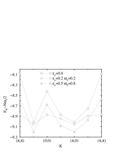
Figure 31: Left panel: Band dispersion for the 2D HtJM on a 16-site lattice ($J=0.4$). Right panel: Spectral weight factor $Z_{\vec{K}}$ as a function of the EP coupling strength $\varepsilon_{p}$ for the different ${\vec{K}}$ vectors of the ten-site lattice: (3,1) (triangles down), (2,4) (squares), (0,0) (circles), and (5,5) (triangles up) [in units of ($\pi/5,\pi/5$)]. The inset shows the narrowing of the coherent bandwidth $\Delta E$ with increasing $\varepsilon_{p}$.

Next we evaluated the wave-function renormalisation factor for different band states,

$$Z_{{\vec{K}}}=\frac{\left|\langle\psi_{0,{\vec{K}}}^{(N_{e}-1)}|\tilde{c}_{{\vec{Q}}-{\vec{K}},\sigma}|\psi_{0,{\vec{Q}}}^{(N_{e})}\rangle\right|^{2}}{\left|\langle\psi_{0,{\vec{Q}}}^{(N_{e})}|\tilde{c}^{\dagger}_{{\vec{Q}}-{\vec{K}},\sigma}\tilde{c}_{{\vec{Q}}-{\vec{K}},\sigma}|\psi_{0,{\vec{Q}}}^{(N_{e})}\rangle\right|^{2}}\,,$$ (48)

where $|\psi_{0,{\vec{Q}}}^{(N_{e}-1)}\rangle$ denotes the one-hole state being lowest in energy in the ${\vec{Q}}$-sector. $Z_{\vec{K}}$ can be taken as a measure of the “contribution” of the hole (dressed at $\varepsilon_{p}=0$ by spin-wave excitations only) to the composite spin/lattice polaron (having total momentum ${\vec{K}}$). The data obtained at weak EP coupling unambiguously confirm the different nature of band states in this regime (see Fig. 31 right panel). We found practically zero-phonon “hole” states at the band minima (${\vec{K}}=(3\pi/5,\pi/5)$, triangles down) and “phonon” states, which are only weakly affected by the hole, around the (flat) band maxima (${\vec{K}}=(\pi,\pi)$, triangles up). With increasing $\varepsilon_{p}$, a strong “mixing” of holes and phonons takes place, whereby both quantum objects completely lose their own identity. Concomitantly $Z_{{\vec{K}}}$ decreases for the “hole–like” states but increases (first of all) for the “phonon-like” states. At large $\varepsilon_{p}$, a small lattice hole polaron is formed, which, according to the numerical data, has an extremely small spectral weight. Then the question arises whether the lattice hole polaron is a “good” quasiparticle in the sense that one can construct a quasiparticle operator, $\tilde{c}_{\vec{K}\sigma}\to\tilde{d}_{\vec{K}\sigma}$, having large spectral weight at the lowest pole in the spectrum. It was demonstrated that such a composite electron/hole-phonon (polaron) operator could be constructed for the Holstein model FLW97 as well as for the $t-J$ model coupled to buckling/breathing modes SPS97 .

In Fig. 32 we show the optical response in the framework of the single-hole 2D HtJM. In the weak EP coupling regime and for phonon frequencies $\omega_{0}>\Delta E_{tJ}$, we recover the main features of the optical absorption spectrum of the 2D $t-J$ model Po91 , i.e., an “anomalous” broad mid-infrared band ($J<\omega<2t$), separated from the Drude peak (${\cal D}\delta(\omega)$; not shown) by a pseudo-gap $\simeq J$, and an “incoherent” tail up to $\omega\simeq 7t$ (cf. Fig. 32 (a)). At larger EP couplings, the overlap with excited multi-phonon states is enlarged and the optical response is enhanced at higher energies. This redistribution of spectral weight from low to high energies can be seen in Fig. 32 (b). As expected the transition to the lattice hole-polaron state, at about $\varepsilon_{p}^{c}(J=0.4,\omega_{0}=0.8)\simeq 2.0$, is accompanied by the development of a broad maximum in $\sigma^{reg}(\omega)$, whereas the Drude weight as well as the low-frequency optical response become strongly suppressed.

Figure 32: Optical conductivity in the 2D HtJM with $J=0.4$. $\sigma^{reg}(\omega)$ and $S^{reg}(\omega)$ were calculated for a ten-site lattice with 15 phonons.

Let us now make contact with the experimentally observed characteristics of the mid-infrared (MIR) spectra in the doped perovskites SAL95 ; Da94 ; TT92 ; AKR94b ). The simple 2D HtJM seems to contain the key ingredients to describe, at least qualitatively, the principal features of the optical absorption spectra of these compounds. This can be seen by comparing Figs. 32 (a) and (b), corresponding to the weak and strong EP coupling situations realized in the cuprate ($\rm La_{2-x}Sr_{x}CuO_{4}$) and nickelate ($\rm La_{2-x}Sr_{x}NiO_{4}$) systems, respectively. The EP interaction ratio $\varepsilon_{p}/t$ in the nickelates is estimated to be about one order of magnitude larger than in the cuprates because of the much smaller transfer amplitude ($t\simeq 0.08$ eV BE93 ). According to the internal structure of the low-spin state, the hopping transport of spin-1/2 composite holes in a spin-1 background is rather complex; implying, within an effective single-band description, a strong reduction of the transition matrix elements LF97 . A striking feature of the absorption spectra in the cuprate superconductors is the presence of a MIR band, centred at about 0.5 eV in lightly doped $\rm La_{2-x}Sr_{x}CuO_{4}$ (which, using $t\sim 0.3$ eV, means that $\omega\sim 1.5$). Such a strong MIR absorption is clearly visible in Fig. 32 (a). Obviously it is quite difficult to distinguish the spectral weight, produced by the dressing of the hole due to the “bag” of reduced antiferromagnetism in its neighbourhood SWZ88 , from other (e.g. hole-phonon coupling) processes that may contribute to the MIR band observed experimentally. The results presented for the HtJM in Fig. 32 (b) support the claims, however, that the MIR band in the cuprates has a mainly “electronic” origin, i.e., the lattice polaron effects are rather weak Da94 . The opposite is true for their isostructural counterpart, the nickelate system, where the MIR absorption band has been ascribed by many investigators to “polaronic” origin BE93 ; Caea97 . Within the HtJM such a situation can be modelled by the parameter set used in Fig. 32 (b). If we fix the energy scale by $t=0.08$ eV, the maximum in the optical absorption is again located at about 0.5 eV. The whole spectrum clearly shows lattice polaron characteristics, where it seems that the lattice hole polarons are of small-to-intermediate size Emi95 . Most notably, we are able to reproduce the experimentally observed asymmetry in the shape of the spectrum, in particular the very gradual decay of $\sigma^{reg}(\omega)$ at high energies. It is worth mentioning that this behaviour cannot be obtained from a simple fit to the analytical expressions derived for the small polaron hopping conductivity BE93 ; Re67 ; SPH91 . Exploiting the f-sum rule we found that there are almost no contributions from band-like carriers in agreement with the experimental findings BE93 ; Caea97 .

Next let us briefly discuss the two-hole problem. In order to study hole-binding effects, we have calculated the hole-hole correlation function

$$C_{ho-ho}(|i-j|)=\langle\psi_{0}(\varepsilon_{p},J)|\tilde{h}_{i}\tilde{h}_{j}|\psi_{0}(\varepsilon_{p},J)\rangle\,.$$ (49)

Results for $C_{ho-ho}(|i-j|)$ are presented in Fig. 33. At weak EP coupling, $C_{ho-ho}(|i-j|)$ becomes maximum at the largest distance of the ten-site lattice, while in the intermediate EP coupling regime the preference is on next NN pairs. As expected, further increasing $\varepsilon_{p}$, the maximum in $C_{ho-ho}(|i-j|)$ is shifted to the shortest possible distance, indicating hole-hole attraction. At $\varepsilon_{p}\gg 1$, the two holes become “self–trapped” sharing a sizeable common lattice distortion, i.e., a nearly immobile hole-bipolaron is formed. The behaviour of $C_{ho-ho}$ is found to be qualitatively similar for higher (lower) phonon frequencies (see inset), except that the crossings of different hole-hole correlation functions occur at larger (smaller) values of $\varepsilon_{p}$, which again shows the importance of both parameter ratios $\lambda=\varepsilon_{p}/2Dt$ and $g=\sqrt{\varepsilon_{p}/\omega_{0}}$.

Figure 33: Non-equivalent hole-hole pair correlation functions $C_{ho-ho}(|i-j|)$ in the two-hole ground state of the HtJM at various $\varepsilon_{p}$. Here 1, 2, and 3 label NN, next NN, and third NN distances, respectively.

Finally let us consider the quarter-filled band case. Here, we have investigated the simpler spinless fermion model (total $S^{z}=S^{z}_{max}$). In accordance with previous approximate treatments based on an inhomogeneous variational Lang-Firsov approach FRWM95 , we found, as the EP coupling increases, evidence for a transition from a free polaron state to a 2D polaronic superlattice, where the holes are self-trapped on every other site. This crossover is signalled by a pronounced peak in the charge structure factor $S_{c}(\pi,\pi)$. To visualise the correlations in this state in more detail, in Fig. 34 we have depicted $C_{ho-ho}(|i-j|)$ and the corresponding hole-phonon density correlation function $C_{ho-ph}(|i-j|)=\langle\psi_{0}|\tilde{h}_{i}b^{\dagger}_{j}b_{j}|\psi_{0}\rangle$ as a function of $|i-j|$. Our exact results clearly show the phonon-dressing of the holes and the tendency towards CDW formation as observed, e.g., in $\rm La_{1.5}Sr_{0.5}NiO_{4}$.

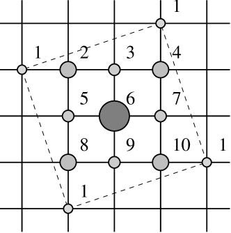
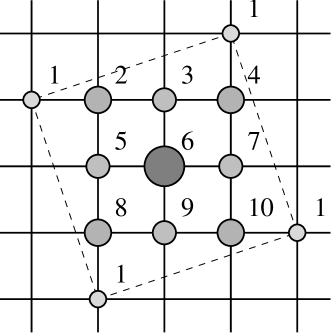
Figure 34: $C_{ho-ho}(|6-j|)$ (left) and $C_{ho-ph}(|6-j|)$ (right) are displayed at $\varepsilon_{p}=3$ and $\omega_{0}=0.8$, where both diameter and gray level of the circles are proportional to the correlation strength.

9.2 Lattice polarons in a generalised double-exchange model

The key elements of the electronic structure of the CMR ($\rm La_{1-x}[Sr,Ca]_{x}MnO_{3}$) compounds are the partially filled 3d states. The cubic environment of the Mn sites within the perovskite lattice results in a crystal field splitting of Mn d-orbitals into $e_{g}$ and $t_{2g}$. In the case of zero doping ($x=0$) there are four electrons per Mn site which fill up the three $t_{2g}$ levels and one $e_{g}$ level, and by Hund’s rule coupling, form a $S=2$ spin state. Doping will remove the electron from the $e_{g}$ level, and by hopping via bridging oxygen sites the resulting holes acquire mobility.

Due to the specific symmetry of the manganese $d$ and oxygen $p$ orbitals, the transfer of the $e_{g}$-electrons shows a pronounced orbital anisotropy. In the limit of large on-site Coulomb ($U$) and Hund ($J_{H}$) interactions the electron transfer is strongly affected by the spin of the core electrons as well. Concentrating on the link between magnetic correlations and transport, early studies on lanthanum manganites attributed the low-$T$ metallic behaviour to Zener’s double-exchange (DE) mechanism Ze51b ; KO72a , which maximises the hopping of a strongly Hund’s rule coupled electron in a polarised spin background.

As discussed above, it has been realized that physics beyond DE is important not only to explain the phase diagram of the manganites but also the CMR transition itself. The orbital degeneracy in the ground state of Mn³⁺ ions connects the system to the lattice, making it susceptible to Jahn-Teller polaron formation. There are two types of lattice distortions which are important in manganites. First the partially filled $e_{g}$ states of the $\rm Mn^{3+}$ ion are Jahn-Teller active, i.e., the system can gain energy from a quadrupolar symmetric elongation of the oxygen octahedra which lifts the $e_{g}$ degeneracy. A second possible deformation is an isotropic shrinking of a $\rm MnO_{6}$ octahedron. This “breathing”-type distortion couples to changes in the $e_{g}$ charge density, i.e., is always associated with the presence of an $\rm Mn^{4+}$ ion.

Restricting the electronic Hilbert space to the large Hund’s rule states given by the spin-$2$ orbital doublet state ${}^{5}E$ [$t_{2}^{3}(^{4}A_{2})e$] for Mn³⁺ (d⁴) and the spin-$\frac{3}{2}$ orbital singlet state ${}^{4}A_{2}$ [$t_{2}^{3}$] for Mn⁴⁺ (d³), within $2^{\rm nd}$ order perturbation theory the following Hamiltonian results (for details of the derivation and notation see Ref. WF02b ; WF04b ):

$$H = H_{\rm DE}+H_{\rm spin-orbital}^{\rm 2^{nd}\;order}+H_{\rm electron-JT}+H_{\rm electron-breathing}+H_{\rm phonon}{}$$ (50)

$$= \sum_{i,\delta,\alpha,\beta}(a_{i,\uparrow}a^{\dagger}_{i+\delta,\uparrow}+a_{i,\downarrow}a^{\dagger}_{i+\delta,\downarrow})\ t^{\delta}_{\alpha\beta}\ c^{\dagger}_{i,\alpha}n_{i,\bar{\alpha}}n_{i+\delta,\bar{\beta}}c_{i+\delta,\beta}{}$$

$$+\sum_{i,\delta,\kappa,\lambda}(J^{\delta}_{\kappa\lambda}\ {\vec{S}}_{i}{\vec{S}}_{i+\delta}+\Delta^{\delta}_{\kappa\lambda})\ P^{\kappa}_{i}P^{\lambda}_{i+\delta}{}$$

$$\,+\bar{g}\sum_{i}\left[(n_{i,\varepsilon}-n_{i,\theta})(b^{\dagger}_{i,\theta}+b_{i,\theta})+(d^{\dagger}_{i,\theta}d_{i,\varepsilon}+d^{\dagger}_{i,\varepsilon}d_{i,\theta})(b^{\dagger}_{i,\varepsilon}+b_{i,\varepsilon})\right]{}$$

$$\,+\tilde{g}\sum_{i}(n_{i,\theta}+n_{i,\varepsilon}-2n_{i,\theta}n_{i,\varepsilon})(b^{\dagger}_{i,a_{1}}+b_{i,a_{1}}){}$$

$$\,+\bar{\omega}_{0}\sum_{i}\left[b^{\dagger}_{i,\theta}b_{i,\theta}+b^{\dagger}_{i,\varepsilon}b_{i,\varepsilon}\right]+\tilde{\omega}_{0}\sum_{i}b^{\dagger}_{i,a_{1}}b_{i,a_{1}}\,.$$

The effective low-energy Hamiltonian $H$ contains Schwinger bosons $a^{(\dagger)}_{i,\mu}$, i.e. $2{\vec{S}}_{i}=a^{\dagger}_{i,\mu}\boldmath{\tau}_{\mu\nu}a_{i,\nu}$ ($\mu,\nu\in\{\uparrow,\downarrow\}$), fermionic holes $c^{(\dagger)}_{i,\alpha}$, phonons $b^{(\dagger)}_{i,\alpha}$ ($\alpha\in\{\theta,\varepsilon\}$), and orbital projectors $P^{\kappa(\lambda)}_{i}$ ($\kappa,\lambda\in\{\xi,\eta,\zeta\}$). In Eq. (50), the first term, being proportional to $t$, corresponds to the DE interaction Ze51b ; KO72a . The second term appears to be a bit more involved, since a rather large number of accessible virtual excitations (proportional to $t^{2}$ and $t_{\pi}^{2}$) contribute (see Refs. WF02b ; WF04b ). However, in all cases it is basically the product of a Heisenberg-type spin interaction and two orbital projectors.

The coupling between the orbital degree of freedom of the $e_{g}$ electrons and the optical phonon modes to lowest order can be modelled by the $E\otimes e$ Jahn-Teller Hamiltonian (third term) and a Holstein-type interaction (fourth term). The energy of the dispersionless optical phonons are given within the harmonic approximation (fifth term).

For analytical methods the above Hamiltonian (50) is far too complex to be understood in full detail, and even its numerical solution on finite lattices is hard. Using high performance computers and the phonon basis optimisation outlined in Sec. 2.2, we were able to calculate the ground-state properties of a small four-site cluster and to address, in particular, short-range correlations between the charge, spin, orbital and lattice degrees of freedom WF02b ; WF04b . (See also [62].) Figures 35 and 36 give a glimpse of these results. We assumed $t=0.4$ eV and $t/t_{\pi}=3$ for the hopping integrals and characterised the magnetic “order” according to the total spin of the ground state.

Undoped manganites ($\rm LaMnO_{3}$, $\rm PrMnO_{3}$) usually exhibit A-type antiferromagnetic order and strong Jahn-Teller distortion of the ideal perovskite structure. The origin of the observed magnetic order has been subject to discussions. While different band structure calculations Saea95 emphasise the importance of lattice distortions for the stability of antiferromagnetism, purely electronic mechanisms were also favoured FO99 . In our microscopic model (50), at $x=0$, only the second and third term will be active, and without EP interaction the competition of the spin-orbital contributions depends sensitively on the values of Coulomb and Hund’s rule coupling. Starting from the ”ferromagnetic” phase increasing either U or g changes the magnetic order of the ground state to ”antiferromagnetism” WF02b (see also Fig. 35 (upper left panel)). At larger EP interaction the system tends to develop static Jahn-Teller distortions, which also fixes the orbital pattern and subsequently the spin order. The change of orbital, spin and phonon correlations is illustrated schematically in Fig. 36 (left panels).

Our numerical calculations corroborate the enhancement of ferromagnetic correlations for the weakly doped case (see Fig. 35, upper left panel; $x=0.25$). However, if strong electron-phonon coupling causes self-trapping of the carriers the spin order switches back to antiferromagnetism. This coincidence can be seen by comparing the total spin of the cluster and the kinetic energy in the ground state, both depicted in the upper panels of Fig. 35. Obviously the change in the magnetic order is accompanied by the appearance of a lattice distortion and a signature in the fluctuation of the bond length ($\propto\langle q_{x/y}^{2}\rangle-\langle q_{x/y}\rangle^{2}$), which reminds of the data measured close to the critical temperature by Booth et al. BBKLCN98 (lower left panel). The orbital orientation at the sites surrounding the hole-site is sketched in Fig. 36 (middle panels). Increasing $g$ isolates the lattice sites, each optimising EP interaction individually and uncorrelated with the neighbours.

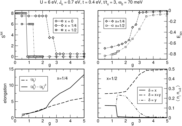
Figure 35: Upper panels: Total spin $S^{tot}$ and kinetic energy $E_{kin}$ as a function of electron-phonon coupling strength $g$ at various doping levels $x$. Lower panels: Expectation values $\langle q_{y}\rangle$ and $\langle q_{y}^{2}\rangle-\langle q_{y}\rangle^{2}$ of the bond length in $y$ direction at $x=1/4$ (left) and density-density correlations at $x=1/2$ (right). Results obtained by ED for the microscopic model (50) on a four site plaquette, where $g=\bar{g}/\omega_{0}$, and $\omega_{0}=\bar{\omega}=\tilde{\omega}$ is assumed WF04b .

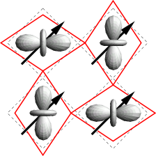
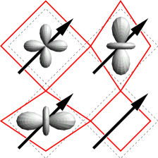
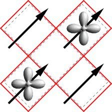
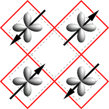
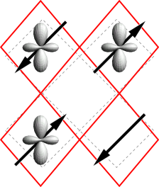
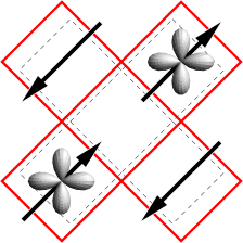
Figure 36: Schematic evolution of charge, spin, orbital and lattice correlation with increasing doping [$x=0$, $x=0.25$ and $x=0.5$ (from left to right)] at rather weak (upper panels) and strong (lower panels) EP couplings.

At half-filling ($x=0.5$) the picture is more involved. Here strong Coulomb and EP interactions tend to order the charges in the diagonal direction, i.e., in an AB-type structure (compare Fig. 35, lower right panel). This allows for a rather large antiferromagnetic spin exchange $\propto t^{2}/J_{H}$. Consequently ferromagnetic order is unstable at much lower values of $g$. The ferromagnetic to antiferromagnetic transition is not connected to charge localisation and causes only a tiny jump of the kinetic energy. Considering the most relevant eigenstate of the bond orbital density matrix, we observe a symmetric order of complex orbitals along the diagonal WF02b . After charge localisation is achieved at large $g$, neighbouring sites are again uncorrelated with respect to orbital ordering and are in some real mixed-orbital state.

Of course, the results of this section will not provide a quantitative analysis or description of the real 3D HTSC and CMR materials. Nevertheless, ED of even such small systems gives valuable insights into the correlations and driving interactions behind the rich phase diagram of the cuprates and manganites. Moreover the above ED data may serve as a benchmark for approximate theories.

10 Conclusions

In summary, we have performed an extensive numerical analysis of the Holstein model. Combining variational Lanczos diagonalisation, density matrix renormalisation group, kernel polynomial expansion, and cluster perturbation theory techniques we solved for properties of the Holstein polaron and bipolaron problems. Numerical solution of the Holstein model means that we determined the ground-state and low-lying excited states with arbitrary precision in the thermodynamic limit for any dimension. Moreover, we calculated the spectral properties (e.g. photoemission and phonon spectra), optical response and thermal transport, as well as the dynamics of polaron formation. Our approach takes into account the full quantum dynamics of the electrons and phonons and yields unbiased results for all electron-phonon interaction strengths and phonon frequencies, but is of particular value in the intermediate-coupling regime, where perturbation theories and other analytical techniques fail.

Most importantly, polaron formation represents a continuous crossover of the ground state. Nevertheless we found indications for a true phase transition in the first excited state, where a polaron plus phonon system changes from unbound at weak electron-phonon coupling to bound at strong coupling. Obviously electron and phonon excitations become intimately, dynamically connected in the process of polaron formation. Concerning ground-state and spectral properties the (quasi-free) electron (small) polaron self-trapping crossover is related to (i) a significant increase of the particle effective mass, (ii) a substantial narrowing of the polaronic band dispersion, and (iii) a strongly suppressed (electronic) quasiparticle residue. At the same time we observe (iv) an enhancement of the (on-site) electron-phonon correlations and the formation of a phonon drag, (v) a loss of kinetic energy, and (vi) a drop of the Drude weight, accompanied (vii) by a maximum in the spectral weight contained in the regular part of the optical response. All these features are found to be much more pronounced in higher dimensions. The study of bipolarons showed that the two-site bipolaron has a significantly reduced mass and isotope effect compared to the on-site bipolaron, and is bound in the strong-coupling regime up to twice the on-site Coulomb repulsion.

Although we have now achieved a rather complete picture of the single Holstein polaron and bipolaron problem (perhaps dispersive phonons, longer-ranged electron-phonon interaction, finite-temperature and disorder effects deserve closer attention), the situation is disconcerting in the case of a finite carrier density. Here a density-driven crossover from large polarons to quasi-free electrons scattered by unbound phonons might occur in the non-adiabatic intermediate coupling regime. Besides electron-phonon coupling competes with sometimes strong electronic correlations, e.g., in quasi-1D MX chains, quasi-2D high-$T_{c}$ superconductors, 3D charge-ordered nickelates, or bulk colossal magneto-resistance manganites. The corresponding microscopic models contain (extended) Hubbard, Heisenberg or double-exchange terms, and maybe also a coupling to orbital degrees of freedom, so that they can hardly be solved even numerically with the same precision as the Holstein model. First exact results obtained for the case of a single carrier on finite lattices give strong evidence that the tendency towards lattice (electron-, hole- or Jahn-Teller-) polaron formation is enhanced in strongly correlated electron systems. A more thorough investigation of these systems materials and models will definitely be a great challenge for solid-state theory in the near future.

References

- (1) L.D. Landau, Phys. Z. Sowjetunion 3, 664 (1933)
- (2) S.I. Pekar, Zh. Eksp. Teor. Fiz. 16, 341 (1946)
- (3) Y.A. Firsov, Polarons (Izd. Nauka, Moscow, 1975)
- (4) E.I. Rashba, in Excitons, ed. by E.I. Rashba, M.D. Sturge (North-Holland, Amsterdam, 1982), p. 543
- (5) Y.E. Perlin, M. Wagner (eds.), The Dynamical Jahn-Teller Effect in Localized Systems. No. 7 in Modern Problems in Condensed Matter Sciences (North-Holland, Amsterdam, 1984)
- (6) A.L. Shluger, A.M. Stoneham, J. Phys. Condens. Matter 5, 3049 (1993)
- (7) H. Fröhlich, Adv. Phys. 3, 325 (1954)
- (8) H. Fröhlich, Fortschr. Phys. 22, 159 (1974)
- (9) J.T. Devreese, this volume, and references therein
- (10) T. Holstein, Ann. Phys. (N.Y.) 8, 325 (1959)
- (11) T. Holstein, Ann. Phys. (N.Y.) 8, 343 (1959)
- (12) F.M. Peeters, J.T. Devreese, Phys. Status Solidi B 112, 219 (1982)
- (13) H. Spohn, Ann. Phys. (N.Y.) 175, 278 (1987)
- (14) H. Löwen, Phys. Rev. B 37, 8661 (1988)
- (15) B. Gerlach, H. Löwen, Rev. Mod. Phys. 63, 63 (1991)
- (16) D. Emin, in Polarons and bipolarons in High– superconductors and related materials, ed. by E.K.H. Salje, A.S. Alexandrov, W.Y. Liang (Cambridge University Press, Cambridge, 1995)
- (17) G. Wellein, H. Fehske, Phys. Rev. B 58, 6208 (1998)
- (18) J. Ranninger, in Polarons in Bulk Materials and Systems With Reduced Dimensionality, International School of Physics Enrico Fermi, vol. 161, ed. by G. Iadonisi, J. Ranninger, G. De Filippis (IOS Press, Amsterdam, 2006), International School of Physics Enrico Fermi, vol. 161, pp. 1–25
- (19) J.T. Devreese, Bull. Soc. Belge de Phys. (Ser. III) 4, 259 (1963)
- (20) N. Tsuda, K. Nasu, A. Yanese, K. Siratori, Electronic Conduction in Oxides (Springer-Verlag, Berlin, 1990)
- (21) Y. Bar-Yam, T. Egami, J.M. de Leon, A.R. Bishop, Lattice Effects in High– Superconductors (World Scientific, Singapore, 1992)
- (22) E.K.H. Salje, A.S. Alexandrov, W.Y. Liang, Polarons and Bipolarons in High Temperature Superconductors and Related Materials (Cambridge University Press, Cambridge, 1995)
- (23) C.H. Chen, S.W. Cheong, A.S. Cooper, Phys. Rev. Lett. 71, 2461 (1993)
- (24) A.J. Millis, Nature 392, 147 (1998)
- (25) M. Jaime, H.T. Hardner, M.B. Salamon, M. Rubinstein, P. Dorsey, D. Emin, Phys. Rev. Lett. 78, 951 (1997)
- (26) T. Egami, in Polarons in bulk materials and systems with reduced dimensionality, International School of Physics Enrico Fermi, vol. 161, ed. by G. Iadonisi, J. Ranninger, G.D. Filipis (IOS Press, Amsterdam, 2006), International School of Physics Enrico Fermi, vol. 161, pp. 101–117
- (27) D. Emin, Adv. Phys. 22, 57 (1973)
- (28) Y. Toyozawa, Prog. Theor. Phys. 26, 29 (1961)
- (29) A.B. Migdal, Sov. Phys. JETP 7, 999 (1958)
- (30) I.G. Lang, Y.A. Firsov, Zh. Eksp. Teor. Fiz. 43, 1843 (1962)
- (31) F. Marsiglio, Physica C 244, 21 (1995)
- (32) A.S. Alexandrov, N.F. Mott, High Temperature Superconductors and Other Superfluids (Taylor & Francis, London, 1994)
- (33) H. Sumi, J. Phys. Soc. Jpn. 36, 770 (1974)
- (34) S. Ciuchi, F. de Pasquale, S. Fratini, D. Feinberg, Phys. Rev. B 56, 4494 (1997)
- (35) F. Marsiglio, Phys. Lett. A 180, 280 (1993)
- (36) A.S. Alexandrov, V.V. Kabanov, D.K. Ray, Phys. Rev. B 49, 9915 (1994)
- (37) E.V.L. de Mello, J. Ranninger, Phys. Rev. B 55, 14872 (1997)
- (38) G. Wellein, H. Röder, H. Fehske, Phys. Rev. B 53, 9666 (1996)
- (39) B. Bäuml, G. Wellein, H. Fehske, Phys. Rev. B 58, 3663 (1998)
- (40) H. De Raedt, A. Lagendijk, Phys. Rev. B 27, 6097 (1983)
- (41) E. Berger, P. Valášek, W. v. d. Linden, Phys. Rev. B 52, 4806 (1995)
- (42) P.E. Kornilovitch, E.R. Pike, Phys. Rev. B 55, R8634 (1997)
- (43) M. Hohenadler, H.G. Evertz, W. von der Linden, Phys. Rev. B 69, 024301 (2004)
- (44) P. Kornilovitch, this volume
- (45) M. Hohenadler, W. von der Linden, this volume
- (46) A.S. Mishchenko, N. Nagaosa, this volume, and references therein
- (47) A.H. Romero, D.W. Brown, K. Lindenberg, J. Chem. Phys 109, 6540 (1998)
- (48) E. Jeckelmann, S.R. White, Phys. Rev. B 57, 6376 (1998)
- (49) C. Zhang, E. Jeckelmann, S.R. White, Phys. Rev. Lett. 80, 2661 (1998)
- (50) E. Jeckelmann, Phys. Rev. B 66, 045114 (2002)
- (51) J.K. Cullum, R.A. Willoughby, Lanczos Algorithms for Large Symmetric Eigenvalue Computations, vol. I & II (Birkhäuser, Boston, 1985)
- (52) R.N. Silver, H. Röder, A.F. Voter, D.J. Kress, J. of Comp. Phys. 124, 115 (1996)
- (53) A. Weiße, G. Wellein, A. Alvermann, H. Fehske, Rev. Mod. Phys. 78, 275 (2006)
- (54) D. Sénéchal, D. Perez, M. Pioro-Ladrière, Phys. Rev. Lett. 84, 522 (2000)
- (55) M. Hohenadler, M. Aichhorn, W. von der Linden, Phys. Rev. B 68, 184304 (2003)
- (56) A. Weiße, H. Fehske, G. Wellein, A.R. Bishop, Phys. Rev. B 62, R747 (2000)
- (57) V. Cautaudella, G.D. Filippis, G. Iadonisi, C.A. Perroini, in Polarons in Bulk Materials and Systems With Reduced Dimensionality, ed. by G. Iadonisi, J. Ranninger, G. De Filippis (IOS Press, Amsterdam, 2006), International School of Physics Enrico Fermi, pp. 119–130
- (58) V. Cataudella, G.D. Filippis, C.A. Perroini, this volume
- (59) S.A. Trugman, L.C. Ku, J. Bonča, J. Supercond. 17, 193 (2004)
- (60) J. Bonča, S.A. Trugman, I. Batistić, Phys. Rev. B 60, 1633 (1999)
- (61) L.C. Ku, S.A. Trugman, J. Bonča, Phys. Rev. B 65, 174306 (2002)
- (62) S. El Shawish, J. Bonča, L.C. Ku, S.A. Trugman, Phys. Rev. B 67, 014301 (2003)
- (63) H. De Raedt, A. Lagendijk, Phys. Rev. Lett. 49, 1522 (1982)
- (64) M. Capone, W. Stephan, M. Grilli, Phys. Rev. B 56, 4484 (1997)
- (65) G. Wellein, H. Fehske, Phys. Rev. B 56, 4513 (1997)
- (66) H. Fehske, D. Ihle, J. Loos, U. Trapper, H. Büttner, Z. Phys. B 94, 91 (1994)
- (67) H. Fehske, G. Wellein, G. Hager, A. Weiße, A.R. Bishop, Phys. Rev. B 69, 165115 (2004)
- (68) J. Bonča, T. Katrašnik, S.A. Trugman, Phys. Rev. Lett. 84, 3153 (2000)
- (69) S. Sykora, A. Hübsch, K.W. Becker, G. Wellein, H. Fehske, Phys. Rev. B 71, 045112 (2005)
- (70) D. Augier, D. Poilblanc, Eur. Phys. J. B 1, 19 (1998)
- (71) E.R. Davidson, J. of Comp. Phys. 17, 87 (1975)
- (72) R.N. Silver, H. Röder, Phys. Rev. E 56, 4822 (1997)
- (73) W. Stephan, Phys. Rev. B 54, 8981 (1996)
- (74) H. Fehske, J. Loos, G. Wellein, Z. Phys. B 104, 619 (1997)
- (75) J. Loos, M. Hohenadler, H. Fehske, J. Phys. Condens. Matter 18, 2453 (2006)
- (76) H. Fehske, A. Alvermann, M. Hohenadler, G. Wellein, in Polarons in Bulk Materials and Systems With Reduced Dimensionality, International School of Physics Enrico Fermi, vol. 161, ed. by G. Iadonisi, J. Ranninger, G. De Filippis (IOS Press, Amsterdam, 2006), International School of Physics Enrico Fermi, vol. 161, pp. 285–296
- (77) A.A. Gogolin, Phys. Status Solidi B 109, 95 (1982)
- (78) D. Emin, T. Holstein, Phys. Rev. Lett. 36, 323 (1976)
- (79) D.R. Jennison, D. Emin, Phys. Rev. Lett. 51, 1390 (1983)
- (80) V.V. Kabanov, O.Y. Mashtakov, Phys. Rev. B 47, 6060 (1993)
- (81) J.A. Kenrow, T.K. Gustafson, Phys. Rev. Lett. 77, 3605 (1996)
- (82) N.H. Ge, et al., Science 279, 202 (1998)
- (83) A. Sugita, T. Saito, H. Kano, M. Yamashita, T. Kobayashi, Phys. Rev. Lett. 86, 2158 (2001)
- (84) S.L. Dexheimer, A.D.V. Pelt, J.A. Brozik, B.I. Swanson, Phys. Rev. Lett. 84, 4425 (2000)
- (85) S. Tomimoto, H. Nansei, S. Saito, T. Suemoto, J. Takeda, , S. Kurita, Phys. Rev. Lett. 81, 417 (1998)
- (86) R.D. Averitt, A.J. Taylor, J. Phys. Condens. Matter 14, R1357 (2002)
- (87) G.P. Donati, G. Rodriguez, A.J. Taylor, J. Opt. Soc. Am. B 17, 1077 (2000)
- (88) B. Krummheuer, V.M. Axt, T. Kuhn, Phys. Rev. B 65, 195313 (2002)
- (89) D.W. Brown, K. Lindenberg, B. J.West, J. Chem. Phys 84, 1574 (1986)
- (90) L.C. Ku, Ph.D. thesis, UCLA (2003)
- (91) D. Emin, Phys. Rev. B 48, 13691 (1993)
- (92) A.S. Alexandrov, N.F. Mott, Polarons and Bipolarons (World Scientic, Singapore, 1995)
- (93) D.C. Worledge, L. Miéville, T.H. Geballe, Phys. Rev. B 57, 15267 (1998)
- (94) G.D. Mahan, Many-Particle Physics (Kluwer Academic/Plenum Publishers, New York, 2000)
- (95) H.G. Reik, D. Heese, J. Phys. Chem. Solids 28, 581 (1967)
- (96) J. Loos, Z. Phys. B 71, 161 (1988)
- (97) Y.A. Firsov, Semiconductors 29, 515 (1995)
- (98) Y.A. Firsov, this volume
- (99) S. Fratini, S. Ciuchi, Phys. Rev. Lett. 91, 256403 (2003)
- (100) S. Fratini, S. Ciuchi, Phys. Rev. B 74, 075101 (2006)
- (101) G. Schubert, G. Wellein, A. Weiße, A. Alvermann, H. Fehske, Phys. Rev. B 72, 104304 (2005)
- (102) E.K. Kudinov, D.N. Mirlin, Y.A. Firsov, Fiz. Tverd. Tela 11, 2789 (1969)
- (103) E.L. Nagaev, Sov. Phys. Solid State 4, 1611 (1963)
- (104) H. Böttger, V.V. Bryksin, Hopping conduction in solids (Akademie Verlag, Berlin, 1985)
- (105) M. Hohenadler, D. Neuber, W. von der Linden, G. Wellein, J. Loos, H. Fehske, Phys. Rev. B 71, 245111 (2005)
- (106) A.S. Alexandrov, this volume
- (107) S. Aubry, this volume
- (108) L. Proville, S. Aubry, Physica (Amsterdam) 133D, 307 (1998)
- (109) M. Capone, M. Grilli, W. Stephan, Eur. Phys. J. B 11, 551 (1999)
- (110) C. Hartinger, F. Mayr, J. Deisenhofer, A. Loidl, T. Kopp, Phys. Rev. B 69, 100403(R) (2004)
- (111) A.S. Alexandrov, P.E. Kornilovitch, Phys. Rev. Lett. 82, 807 (1999)
- (112) J.T. Devreese, J. Tempere, Phys. Rev. B 64, 104504 (2001)
- (113) H. Rietschel, J. Low Temp. Phys. 95, 293 (1994)
- (114) R.P. Sharma, L.E. Rehn, P.M. Baldo, J.Z. Lin, Phys. Rev. Lett. 62, 2869 (1989)
- (115) T. Haga, et al., Phys. Rev. B 41, 826 (1990)
- (116) T. Egami, et al., in Electronic Structure and Mechanisms of High Temperature Superconductivity, ed. by J. Ashkenazi, G. Vezzoli (Plenum Press, New York, 1991)
- (117) Y.H. Kim, et al., Phys. Rev. B 38, 6478 (1988)
- (118) J.D. Jorgenson, Physics Today 44, 34 (1991)
- (119) J. Zhong, H.B. Schüttler, Phys. Rev. Lett. 69, 1600 (1992)
- (120) D. Mihailović, C.M. Foster, K. Voss, A.J. Heeger, Phys. Rev. B 42, 7989 (1990)
- (121) P. Calvani, Solid State Commun. 91, 113 (1994)
- (122) J.P. Falck, A. Levy, M.A. Kastner, R.J. Birgenau, Phys. Rev. B 48, 4043 (1993)
- (123) O. Rösch, O. Gunnarson, X. Zhou, T. Yoshida, T. Sasagawa, A. Fujimori, Z. Hussain, Z.X. Shen, S. Uchida, Phys. Rev. Lett. 95, 227002 (2005)
- (124) G. Verbist, F.M. Peeters, J.T. Devreese, Physica Scripta T 39, 66 (1991)
- (125) D. Emin, Phys. Rev. B 45, 5525 (1992)
- (126) D. Emin, Phys. Rev. Lett. 72, 1052 (1994)
- (127) A.S. Alexandrov, A.B. Krebs, Usp. Fiz. Nauk 162, 1 (1992)
- (128) A.S. Alexandrov, J. Ranninger, Physica C 198, 360 (1992)
- (129) A.S. Alexandrov, A.M. Bratkovsky, N.F. Mott, E.K.H. Salje, Physica C 215, 359 (1993)
- (130) J.E. Hirsch, Phys. Rev. B 47, 5351 (1993)
- (131) N.F. Mott, J. Phys. Condens. Matter 5, 3487 (1993)
- (132) A.S. Alexandrov, N.F. Mott, Int. J. Mod. Phys. B 8, 2075 (1994)
- (133) J. Ranninger, Acta Phys. Pol. A 85, 89 (1994)
- (134) G. Iadonisi, V. Cataudella, D. Ninno, M.L. Chiofalo, Phys. Lett. A 196, 359 (1995)
- (135) X.X. Bi, P.C. Eklund, Phys. Rev. Lett. 70, 2625 (1993)
- (136) V.I. Anisimov, M.A. Korotin, J. Zaanen, O.K. Andersen, Phys. Rev. Lett. 68, 345 (1992)
- (137) G. Zhao, K. Conder, H. Keller, K.A. Müller, Nature 381, 676 (1996)
- (138) S. Jin, T.H. Tiefel, M. McCormack, R.A. Fastnach, R. Ramesh, L.H. Chen, Science 264, 413 (1994)
- (139) P.B. Allen, V. Perebeinos, Phys. Rev. B 61, 10747 (1999)
- (140) S.J.L. Billinge, T. Proffen, V. Petkov, J.L. Sarrao, S. Kycia, Phys. Rev. B 62, 1203 (2000)
- (141) A.S. Alexandrov, A.M. Bratkovsky, Phys. Rev. Lett. 82, 141 (1999)
- (142) P. Calvani, P. Dore, S. Lupi, A. Paolone, P. Maselli, P. Guira, B. Ruzicka, S.W. Cheong, W. Sadowski, J. Supercond. 10, 293 (1997)
- (143) J.D. Lee, B.I. Min, Phys. Rev. B 55, 12454 (1997)
- (144) M. Quijada, J. Černe, J.R. Simpson, H.D. Drew, K.H. Ahn, A.J. Millis, R. Shreekala, R. Ramesh, M. Rajeswari, T. Venkatesan, Phys. Rev. B 58, 16093 (1998)
- (145) K.H. Kim, J.H. Jung, T.W. Noh, Phys. Rev. Lett. 81, 1517 (1998)
- (146) K.A. Müller, J. Supercond. 12, 3 (1999)
- (147) D.S. Dessau, T. Saitoh, C.H. Park, Z.X. Shen, P. Villella, N. Hamada, Y. Morimoto, Y. Tokura, J. Supercond. 12, 273 (1999)
- (148) A. Weiße, J. Loos, H. Fehske, Phys. Rev. B 68, 024402 (2003)
- (149) M. Jaime, M.B. Salamon, M. Rubinstein, R.E. Treece, J.S. Horwitz, D.B. Chrisey, Phys. Rev. B 54, 11914 (1996)
- (150) T.T.M. Palstra, A.P. Ramirez, S.W. Cheong, B.R. Zegarski, P. Schiffer, J. Zaanen, Phys. Rev. B 56, 5104 (1997)
- (151) S.J.L. Billinge, R.G. DiFrancesco, G.H. Kwei, J.J. Neumeier, J.D. Thompson, Phys. Rev. Lett. 77, 715 (1996)
- (152) S. Shimomura, N. Wakabayashi, H. Kuwahara, Y. Tokura, Phys. Rev. Lett. 83, 4389 (1999)
- (153) L. Vasiliu-Doloc, S. Rosenkranz, R. Osborn, S.K. Sinha, J.W. Lynn, J. Mesot, O.H. Seeck, G. Preosti, A.J. Fedro, J.F. Mitchell, Phys. Rev. Lett. 83, 4393 (1999)
- (154) P. Dai, J.A. Fernandez-Baca, N. Wakabayashi, E.W. Plummer, Y. Tomioka, Y. Tokura, Phys. Rev. Lett. 85, 2553 (2000)
- (155) D. Louca, T. Egami, E.L. Brosha, H. Röder, A.R. Bishop, Phys. Rev. B 56, R8475 (1997)
- (156) G.M. Zhao, V. Smolyaninova, W. Prellier, H. Keller, Phys. Rev. Lett. 84, 6086 (2000)
- (157) H. Fehske, H. Röder, A. Mistriotis, H. Büttner, J. Phys. Condens. Matter 5, 3635 (1993)
- (158) R. Fehrenbacher, Phys. Rev. B 49, 12230 (1994)
- (159) A. Sherman, M. Schreiber, Phys. Rev. B 52, 10621 (1995)
- (160) E. Dagotto, Rev. Mod. Phys. 66, 763 (1994)
- (161) H. Fehske, H. Röder, G. Wellein, A. Mistriotis, Phys. Rev. B 51, 16582 (1995)
- (162) T. Sakai, D. Poilblanc, D.J. Scalapino, Phys. Rev. B 55, 8445 (1997)
- (163) D. Poilblanc, Phys. Rev. B 44, 9562 (1991)
- (164) D.B. Tanner, T. Timusk, in Physical Properties of High–Temparature Superconductors III, ed. by D.M. Ginsberg (World Scientific, Singapore, 1992), p. 363
- (165) A.S. Alexandrov, V.V. Kabanov, D.K. Ray, Physica C 224, 247 (1994)
- (166) J. Loos, H. Fehske, Phys. Rev. B 56, 3544 (1997)
- (167) J.R. Schrieffer, X.G. Wen, S.C. Zhang, Phys. Rev. Lett. 60, 944 (1988)
- (168) H.G. Reik, Z. Phys. 203, 364 (1967)
- (169) Y.Y. Suzuki, P. Pincus, A.J. Heeger, Phys. Rev. B 44, 7127 (1991)
- (170) C. Zener, Phys. Rev. 82, 403 (1951)
- (171) K. Kubo, N. Ohata, J. Phys. Soc. Jpn. 33, 21 (1972)
- (172) A. Weiße, H. Fehske, Eur. Phys. J. B 30, 487 (2002)
- (173) A. Weiße, H. Fehske, New J. Phys. 6, 158 (2004)
- (174) D.D. Sarma, N. Shanthi, S.R. Barman, N. Hamada, H. Sawada, K. Terakura, Phys. Rev. Lett. 75, 1126 (1995)
- (175) L.F. Feiner, A.M. Oleś, Phys. Rev. B 59, 3295 (1999)
- (176) C.H. Booth, F. Bridges, G.H. Kwei, J.M. Lawrence, A.L. Cornelius, J.J. Neumeier, Phys. Rev. Lett. 80, 853 (1998)