Numerical study of subdiffusion equation

Abstract

We present a numerical procedure of solving the subdiffusion equation with Caputo fractional time derivative. On the basis of few examples we show that the subdiffusion is a ’long time memory’ process and the short memory principle should not be used in this case.

PACS numbers: 02.50.Ey, 05.10.-a, 02.60.Cb

1 Introduction

The subdiffusion equation is of fractional order with respect to the time variable. Unfortunately, the exact solutions are known only for relatively simple systems, similarly to the normal diffusion case. In more complicated situations such as a system with subdiffusion coefficient depending on concentration, inhomogenous fractional subdiffusive system or subdiffusion-reaction system, one needs a numerical procedure to solve of the equation. Usually the subdiffusion equation contains the Riemann-Liouville fractional time derivative of the order $1-\alpha$ ($\alpha$ denotes here the subdiffusion parameter), which is not convenient for physical interpretation of initial conditions. To get the subdiffusion equation with initial conditions which have simple interpretation, one can use the subdiffusion equation with the Caputo fractional time derivative of the order $\alpha$. As far as we know, there is a numerical method to solve the subdiffusion equation with the Riemann-Liouville fractional time derivative [2]. The equation with Caputo derivative has been numerically studied only within the time fractional discrete random walk [3].

Subdiffusion is a process with the time memory. There arises a practical problem with the memory length, which extends to $-\infty$. To omit the difficulty Podlubny [4, 5] postulated to apply the short memory principle which assumes that the relatively small memory length is sufficient to obtain satisfactorily accuracy of numerical solutions for sufficiently long times. However, as shown here, the method produces significant differences between the numerical and exact solutions. In this paper we present a numerical procedure of solving the subdiffusion equation with Caputo derivative, which is based on the fractional difference approach, and we briefly study the efficiency of the short memory principle for this case.

2 Subdiffusion equation

The transport process is described by the subdiffusion equation [1]

$$\frac{\partial C(x,t)}{\partial t}=D_{\alpha}\frac{{}^{RL}\partial^{1-\alpha}}{\partial t^{1-\alpha}}\frac{\partial^{2}C(x,t)}{\partial x^{2}},$$ (1)

where $0<\alpha<1$, $C(x,t)$ denotes the concentration of transported substance, the Riemann-Liouville fractional time derivative is defined for $\alpha>0$ as

$$\frac{{}^{RL}\partial^{\alpha}f(t)}{\partial t^{\alpha}}=\frac{1}{\Gamma(n-\alpha)}\frac{\partial^{n}}{\partial t^{n}}\int_{0}^{t}dt^{\prime}\frac{f(t^{\prime})}{(t-t^{\prime})^{1+\alpha-n}},$$ (2)

where the integer number $n$ fulfills the relation $n-1<\alpha\leq n$.

The presence of time derivatives on both sides of Eq. (1) is not convenient for numerical calculations. To simplify the numerical procedure we rewrite the Eq. (1) in the form

$$\frac{{}^{C}\partial^{\alpha}C(x,t)}{\partial t^{\alpha}}=D_{\alpha}\frac{\partial^{2}C(x,t)}{\partial x^{2}},$$ (3)

where the fractional time derivative on the left-hand side of Eq. (3) is now Caputo derivative defined by the relation

$$\frac{{}^{C}\partial^{\alpha}f(t)}{\partial t^{\alpha}}=\frac{1}{\Gamma(\alpha-n)}\int_{0}^{t}dt^{\prime}\frac{f^{(n)}(t^{\prime})}{(t-t^{\prime})^{1+\alpha-n}},$$ (4)

$f^{(n)}$ denotes the derivative of natural order $n$.

We note that the Laplace transform of the Caputo fractional derivative involves values of the function $f$ and its derivatives of natural order at $t=0$ while Laplace transform of the Riemann-Liouville fractional derivative includes the fractional derivatives of $f$ at $t=0$. Thus, the physical interpretation of initial conditions in the former case is clear in contrast to the latter one [4]. So, it is more convenient to set the initial conditions for the equation with Caputo derivative than for the equation with Riemann-Liouville one.

3 Numerical procedure

3.1 Fractional derivatives

To numerically solve the normal diffusion equation one usually substitutes the time derivative by the backward difference $\frac{\partial f(t)}{\partial t}\simeq\frac{f(t)-f(t-\Delta t)}{\Delta t}$. In the presented procedure we proceed in a similar way. For that purpose we use the Grünwald-Letnikow fractional derivative, which is defined as a limit of a fractional-order backward difference [4]

$$\frac{{}^{GL}\partial^{\alpha}f(t)}{\partial t^{\alpha}}=\lim_{\Delta t\rightarrow 0}(\Delta t)^{-\alpha}\sum_{r=0}^{[\frac{t}{\Delta t}]}(-1)^{r}\left(\begin{array}[]{c}\alpha\\ r\end{array}\right)f(t-r\Delta t),$$ (5)

where $\alpha>0$, $[x]$ means the integer part of $x$ and

$$\left(\begin{array}[]{c}\alpha\\ r\end{array}\right)=\frac{\Gamma(\alpha+1)}{r!\Gamma(\alpha-r+1)}=\frac{\alpha(\alpha-1)(\alpha-2)\cdot\ldots\cdot[\alpha-(r-1)]}{1\cdot 2\cdot 3\cdot\ldots\cdot r}.$$

When the function $f(t)$ of positive argument has continuous derivatives of the integer order $0,1,\ldots,n$, the Riemann-Liouville definition (2) is equivalent to the Grünwald-Letnikow one [4]. So, we can take

$$\frac{{}^{RL}\partial^{\alpha}f(t)}{\partial t^{\alpha}}=\frac{{}^{GL}\partial^{\alpha}f(t)}{\partial t^{\alpha}}.$$ (6)

The relation between Riemann-Liouville and Caputo derivatives is more complicated and reads as [4]

$$\frac{{}^{RL}\partial^{\alpha}f(t)}{\partial t^{\alpha}}=\frac{{}^{C}\partial^{\alpha}f(t)}{\partial t^{\alpha}}+\sum_{k=0}^{n-1}\Phi_{k-\alpha+1}(t)f^{(k)}(0),$$ (7)

where

$$\Phi_{q+1}(t)=\left\{\begin{array}[]{cc}\frac{t^{q}}{\Gamma(q+1)}&t>0\\ 0&t\leq 0\end{array}\right..$$ (8)

From Eqs. (5)-(8) we can express the Caputo fractional derivative in terms of the fractional-order backward difference [4]

$$\frac{{}^{C}\partial^{\alpha}f(t)}{\partial t^{\alpha}}=\lim_{\Delta t\rightarrow 0}(\Delta t)^{-\alpha}\sum_{r=0}^{[\frac{t}{\Delta t}]}(-1)^{r}\left(\begin{array}[]{c}\alpha\\ r\end{array}\right)f(t-r\Delta t)-\frac{1}{t^{\alpha}\Gamma(1-\alpha)}f(0).$$ (9)

3.2 Algorithm

The standard way to approximate of the fractional derivative, which is useful for numerical calculations, is to omit the limit in Eq. (9) and to change the infinite series occurring in (9) to the finite one

$$\frac{{}^{C}\partial^{\alpha}f(t)}{\partial t^{\alpha}}\simeq(\Delta t)^{-\alpha}\sum_{r=0}^{L}(-1)^{r}\left(\begin{array}[]{c}\alpha\\ r\end{array}\right)f(t-r\Delta t)-\frac{1}{t^{\alpha}\Gamma(1-\alpha)}f(0),$$ (10)

where arbitrary chosen parameter $L$ is called the memory length. Substituting Eq. (10) to Eq. (3) and using the following approximation of the second order derivative

$$\frac{\partial^{2}f(x)}{\partial x^{2}}\simeq\frac{f(x+\Delta x)-2f(x)+f(x-\Delta x)}{(\Delta x)^{2}},$$ (11)

after simple calculation we obtain

$$C(x,t)=-\sum_{r=1}^{L}(-1)^{r}\frac{\alpha(\alpha-1)(\alpha-2)\cdot\ldots\cdot[\alpha-(r-1)]}{1\cdot 2\cdot 3\cdot\ldots\cdot r}C(x,t-r\Delta t)$$

$$+\frac{1}{t^{\alpha}\Gamma(1-\alpha)}C(x,0)+D_{\alpha}\frac{(\Delta t)^{\alpha}}{(\Delta x)^{2}}[C(x+\Delta x,t-\Delta t)$$ (12)

$$-2C(x,t-\Delta t)+C(x-\Delta x,t-\Delta t)].$$

There arise a problem with the choice of initial conditions. We choose the initial conditions only for $t=0$ assuming that the concentration given for earlier moments $t<0$ does not influence the process for $t>0$. This assumption is in agreement with the procedure of solving the equations with Caputo fractional derivative where the initial conditions are determined only at $t=0$ for the derivatives of natural order $f^{(n)}(t)|_{t=0}$, $n=0,1,\ldots,[\alpha]$ (here $f^{(0)}\equiv f$). In our considerations we have $0<\alpha<1$, hence it is enough to set $C(x,0)$ as the initial condition.

Starting with the initial condition $C(x,0)$ we will find the time iterations $C(x,t_{s}\Delta t)$ for $t_{s}=1,2,...,t_{s,max}$. When the number of time steps $t_{s}$ is less then the memory length $L$ then we put $L=t_{s}$ in the series occurring in Eq. (3.2), otherwise the memory length is equal to $L$.

4 Numerical results

To test the numerical procedure we are going to compare the numerical solutions of the subdiffusion equation with the exact analytical ones. For that purpose we choose the homogenous system with the initial concentration

$$C(x,0)=\left\{\begin{array}[]{cc}C_{0}&x<0\\ 0&x\geq 0\end{array}\right..$$ (13)

The solution of the subdiffusion equation (3) with the initial condition (13) is following [6]

$$C(x,t)=\left\{\begin{array}[]{lc}C_{0}-\frac{C_{0}}{\alpha}H^{10}_{11}\left(\frac{(-x)^{2/\alpha}}{D_{\alpha}^{1/\alpha}t}\left|\begin{array}[]{cc}1&1\\ 0&2/\alpha\end{array}\right.\right)&x<0\\ &\\ \frac{C_{0}}{\alpha}H^{10}_{11}\left(\frac{x^{2/\alpha}}{D_{\alpha}^{1/\alpha}t}\left|\begin{array}[]{cc}1&1\\ 0&2/\alpha\end{array}\right.\right)&x\geq 0\end{array}\right.,$$ (14)

where $H$ denotes the Fox function, which can be expressed by the series [7]

$$H^{10}_{11}\left(\frac{x^{2/\alpha}}{D_{\alpha}^{1/\alpha}t}\left|\begin{array}[]{cc}1&1\\ 0&2/\alpha\end{array}\right.\right)=\frac{2}{\alpha}\sum_{k=0}^{\infty}\frac{1}{k!\Gamma\left(1-k\alpha/2\right)}\left(-\frac{x}{\sqrt{D_{\alpha}}t^{\alpha/2}}\right)^{k}\;.$$ (15)

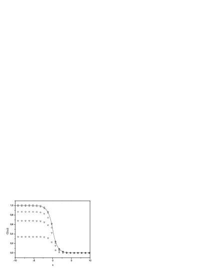
Figure 1: The concentration profiles $C(x,t)$ calculated for $\alpha=0.5$, $D_{\alpha}=0.25$, $t_{s,max}=100$ and with different memory length $L=100(\diamondsuit)$, $80(\triangle)$, $50(\circ)$, $30(\nabla)$, and $10$; continuous line represents the exact analytical solution.

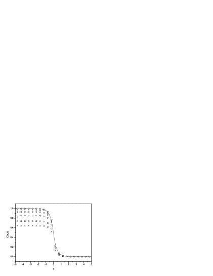
Figure 2: The concentration profiles obtained for $\alpha=0.2$, $D_{\alpha}=0.2$, $t_{s,max}=50$ and with memory length $L=50(\diamondsuit)$, $40(\triangle)$, $30(\circ)$, $20(\nabla)$, $10$, and $5(\times)$.

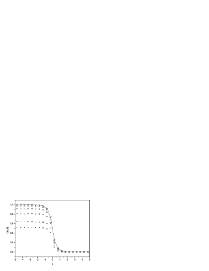
Figure 3: The concentration profiles calculated for $\alpha=0.3$, $D_{\alpha}=0.1$, time $t_{s,max}=50$ and with memory length $L=50(\diamondsuit)$, $40(\triangle)$, $30(\circ)$, $20(\nabla)$, $10$, and $5(\times)$.

The results of numerical calculations and the analytical solutions are shown in the plots. In Figures 1-3 we present the numerical solutions of the subdiffusion equation for different values of $t$, $\alpha$, and $D_{\alpha}$. In each case we present the plot of analytical solution (continuous line) and numerical solutions calculated for different memory length $L$ (symbols without line). The time and the memory length are given as the number of all time steps $t_{s,max}$, which corresponds to the ’real time’ $t$ by the relation $t=\Delta t\cdot t_{s,max}$. In all cases we take $C_{0}=1$, $\Delta t=0.1$ and $\Delta x=0.5$ (all quantities are given in arbitrary units); to calculate the analytical solutions (14) we took 100 first terms in the series occurring in (15). We can see that the memory length determines the accuracy of numerical solutions.

5 Final remarks

We have presented the procedure to numerically solve the subdiffusion equation with Caputo fractional time derivative. The choice of the equation in such a form is not accidental since the interpretation of the initial condition in this case is simpler than in the equation with Riemann-Liouville derivative. In all considered cases the numerical solutions coincide with the analytical ones. In the studies [4, 5] the ’short memory principle’ was postulated. According to this principle, the fractional derivative is approximated by the fractional derivative with moving lower limit $t-L$, where $L$ is the ’memory length’. The examples presented in [4] suggest that the $L=50$ time steps gives a good approximation for times of the order of $t_{s}\sim 100$ time steps. However, the results presented here show that this memory length is not sufficient for the subdiffusion case. Our analysis demonstrate that the memory length should be longer than about 80 per cent of the value of time variable.

References

- [1] R. Metzler, J. Klafter, Phys. Rep. 339, 1 (2000); J. Phys. A37, R161 (2004).
- [2] S.B. Yuste, L. Acedo, SIAM J. Numer. Anal. 42, 1862 (2005) (and references therein).
- [3] R. Gorenflo, F. Mainardi, D. Moretti, P. Paradisi, Nonlin. Dyn. 29, 129 (2002).
- [4] I. Podlubny, Fractional differential equations; Academic Press, San Diego 1999.
- [5] I. Podlubny, L. Dorcak, I. Kostial, Proc. 36th IEEE CDC, San Diego 1997, p. 4985 .
- [6] T. Kosztołowicz, K. Dworecki, S. Mrówczyński, Phys. Rev. E71, 041105 (2005).
- [7] T. Kosztołowicz, J. Phys. A: Math. Gen. 37, 10779 (2004).