A novel method for measuring the bending rigidity of model lipid membranes by simulating tethers

Abstract

The tensile force along a cylindrical lipid bilayer tube is proportional to the membrane’s bending modulus and inversely proportional to the tube radius. We show that this relation, which is experimentally exploited to measure bending rigidities, can be applied with even greater ease in computer simulations. Using a coarse-grained bilayer model we efficiently obtain bending rigidities that compare very well with complementary measurements based on an analysis of thermal undulation modes. We furthermore illustrate that no deviations from simple quadratic continuum theory occur up to a radius of curvature comparable to the bilayer thickness.

I Introduction

Bilayer-forming lipids are the basic structural component of biological cell membranes. In these amphiphilic molecules a hydrophilic group is connected to one or two hydrophobic hydrocarbon chains. When dissolved into water they spontaneously assemble into a variety of structures. In Nature lipid bilayers form the outer plasma membrane of cells as well as the walls of the different cellular compartments and organelles, such as the endoplasmic reticulum, the Golgi apparatus, and the nucleus. Lodish .

Lipid bilayer membranes display interesting physics on many different length- and time-scales. On atomistic length scales this includes questions such as: How do lipid tail length and its degree of saturation influence the bilayer state, how does a specific hydrophilic head group facilitate solubilization, or how can water permeate the hydrophobic region? On somewhat larger scales the embedding of trans-membrane proteins or bilayer fusion are being studied. And on scales exceeding several times the bilayer thickness, one may ask how vesicles are formed and what shape they have, which forces go along with a particular bilayer geometry, or how the demixing of a multicomponent membrane can trigger morphology changes. These different sets of questions require different techniques for their treatment. In the present article we focus on the physics happening on the large scale end, i. e., on the continuum level that may be employed on length scales beyond a few tens of nanometers, when a membrane may be viewed as a twodimensional fluid elastic sheet.

As is typical in any coarse-graining scheme, many details pertaining the a physical system on a given scale get condensed into a few effective parameters on a larger level. Indeed, on the continuum level what remains of all lipid detail are three material parameters – two moduli describing the softest deformation, which is bending, and one length scale describing a spontaneous curvature. The respective Hamiltonian, proposed in the early 70’s Canham70 ; Helfrich1 ; Evans74 can be written as a surface integral over the entire membrane:

$$E=\int{\operatorname{d}}A\,\Big{\{}\frac{1}{2}\kappa(K-C_{0})^{2}+\bar{\kappa}K_{\text{G}}\Big{\}}\ .$$ (1)

Here, the extrinsic curvature $K=1/R_{1}+1/R_{2}$ is the sum of the two local principal curvatures, and the Gaussian curvature $K_{\text{G}}=1/R_{1}R_{2}$ is their product. The inverse length $C_{0}$ indicates any spontaneous curvature which the bilayer might have, so the first term quadratically penalizes deviations of the local extrinsic curvature from $C_{0}$. The two moduli $\kappa$ and $\bar{\kappa}$ belonging to the two quadratic curvature expressions are referred to as bending modulus and saddle splay modulus, respectively. If the membrane has two identical leaflets, $C_{0}=0$ by symmetry, a situation which does seldomly hold for biological membranes but very frequently for artificial lipid bilayers and vesicles. Furthermore, since the surface integral over the Ricci scalar $R$ can be expressed as a boundary integral plus a topological term, the second term in Eqn. (1) most often only contributes a constant and can then be ignored. Under these conditions there remains only a single physical parameter characterizing the membrane, the bending modulus $\kappa$, and it is thus the most important one to determine.

Bending rigidities have been measured experimentally by various techniques Brochard ; Webb ; Bothorel ; Evans1 ; Evans2 ; Ipsen1 ; Ipsen2 ; Waugh ; DaiSheetz95 ; Evans3 ; Bassereau , all ultimately based on one of two general approaches: One may either utilize the dependence of thermal undulations on a membrane’s rigidity, or measure the force needed to actively bend it. The traditional realization of the first approach is to monitor the fluctuations of vesicles as a function of wavelength by light microscopy, a method termed “flicker spectroscopy” Brochard ; Webb ; Bothorel . A related experimental method is based on micro-pipette manipulation techniques. There, the flicker spectrum is successively suppressed by increasing the pipette pressure, and the bending rigidity can then be obtained from the low-tension regime of the tension-area curve Evans1 ; Evans2 ; Ipsen1 ; Ipsen2 . The second approach is typically implemented by measuring the force needed to pull nanoscale bilayer tubes (tethers) from vesicles Waugh ; DaiSheetz95 ; Evans3 ; Bassereau . Since the formation of a tube involves the creation of a high curvature, the work to pull a tether is basically done against bending energy, hence the modulus $\kappa$ can be determined from it.

Determination of the bending rigidity is of course equally important in computer simulation studies of lipid bilayers, and the spectrum of available methods is the same. However, by far the most common approach in simulations is flicker spectroscopy, both for atomistic simulations LindahlEdholm00 ; Marrink1 ; BoPadeBr05 as well as for various coarse grained methods BoPadeBr05 ; Lipowsky2 ; Farago03 ; Stevens04 ; Ira1 ; Ira2 ; BranniganBrown06 . Only recently den Otter and Briels have proposed a method by which constraining forces are applied to actively deform the membrane Briels1 , and Farago and Pincus have proposed a scheme based on the change in free energy of deforming the bilayer FaragoPincus04 . Unfortunately, both active methods involve significant technical and conceptual sophistication. This may explain why the idea is not commonly employed, despite the fact that particularly for stiff membranes fluctuation based schemes encounter difficulties (in experiments as well as in simulations), because the thermally excited amplitudes decrease with bending modulus and become difficult to resolve at some point.

In the present article we propose an alternative simulation approach for studying the curvature elasticity of membranes by an active deformation. Our setup essentially involves measuring the force necessary to hold a membrane tether, and it is thus conceptually identical to its experimental “counterpart”. As we will see, complications of earlier active schemes are avoided, and the simulations are very easy to perform and analyze. We apply this method to a recently proposed coarse-grained solvent-free simulation model Ira1 ; Ira2 and find results that agree very well with data from the analysis of the thermal fluctuations. Moreover, the method permits us to check, up to which curvatures the quadratic model from Eqn. (1) remains valid. Our results indicate that curvature radii close to the bilayer thickness can be imposed without noticeable deviations from Eqn. (1). While the precise location for the breakdown of quadratic theory may well be model dependent, its validity up to length scales comparable to bilayer thickness is in agreement with experimental findings Bassereau .

II Curvature Elasticity

In this section we first briefly review the fluctuation approach towards bilayer elasticity and discuss some of its difficulties. We then introduce the alternative scheme based on holding a membrane tether.

II.1 Flicker spectroscopy

The energy expression in Eqn. (1) requires knowledge of the local membrane curvature. For essentially flat membranes, which can be described by specifying their height $h(x,y)$ above some reference plane (“Monge-parametrization”), this curvature is given by

$$K={\boldsymbol{\nabla}}\cdot\left(\frac{{\boldsymbol{\nabla}}h}{\sqrt{1+({\boldsymbol{\nabla}}h)^{2}}}\right)\stackrel{{\scriptstyle|{\boldsymbol{\nabla}}h|\ll 1}}{{\approx}}\Delta h\ ,$$ (2)

where ${\boldsymbol{\nabla}}$ is the two-dimensional nabla operator on the base plane. The approximation in the second step is the lowest order term in a small gradient expansion. On this level the Hamiltonian (1) becomes quadratic and can be diagonalized by Fourier transformation. Assuming an $L\times L$ membrane patch with periodic boundary conditions, and writing $h({\boldsymbol{r}})=\sum_{{\boldsymbol{q}}}h_{{\boldsymbol{q}}}\,{\operatorname{e}}^{{\operatorname{i}}\,{\boldsymbol{q}}\cdot{\boldsymbol{r}}}$, one finds

$$E=\frac{1}{2}L^{2}\sum_{\boldsymbol{q}}|h_{\boldsymbol{q}}|^{2}(\kappa q^{4}+\Sigma q^{2})\ ,$$ (3)

where we for completeness also added a surface tension term, $\Sigma$ times excess area. From the equipartition theorem we then see that the mean squared amplitude of each mode, i. e., the fluctuation spectrum or the static structure factor, is given by

$$\langle|h_{\boldsymbol{q}}|^{2}\rangle=\frac{k_{\operatorname{B}}T}{L^{2}\big{(}\kappa q^{4}+\Sigma q^{2})}\ .$$ (4)

A fit of the fluctuation spectrum measured in the simulation to this expression yields bending modulus $\kappa$ and tension $\Sigma$. Since for wave vectors smaller than $q_{\min}\simeq\sqrt{\Sigma/\kappa}$ the fluctuations are tension dominated, it is best to simulate at zero tension in order to avoid unnecessary damping of the most relevant modes. In this case the expression $1/(q^{4}\langle|h_{\boldsymbol{q}}|^{2}\rangle L^{2})$ approaches $\kappa$ in the limit $q\rightarrow 0$, as is illustrated in Fig. 1 for a model simulation Ira1 ; Ira2 described in more detail below. For wave vectors approaching $q_{\max}\simeq 2\pi/w$, where $w$ is the bilayer thickness, discrete lipid fluctuations such as protrusions require a more careful analysis BranniganBrown06 .

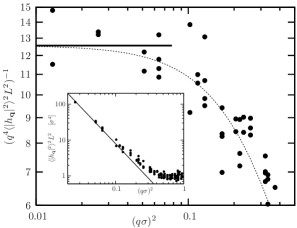
Figure 1: Flicker spectrum of a fluctuating membrane, plotted in such a way that in the limit $q\rightarrow 0$ the expression approaches $\kappa$, see Eqn. (4) The dashed line is a fit of the form $(k_{\operatorname{B}}T/\kappa+c_{1}\,(q\sigma)^{c_{2}})^{-1}$ which helps to find the asymptotic value; the inset shows the unscaled spectrum. The fit leads to $\kappa=12.5\,k_{\operatorname{B}}T$, with an error estimated to be $\pm 1\,k_{\operatorname{B}}T$. The system is the same lipid bilayer model Ira1 ; Ira2 that will be used for the tethers, see below.

There are clear limitations for the calculation of $\kappa$ using thermal fluctuations. The first and obvious one is that large values of $\kappa$ lead to very small amplitudes. Considering ($i$) that $\kappa/k_{\operatorname{B}}T$ is typically of order 10 and ($ii$) how strongly the amplitudes decay with increasing wave vector, one realizes that it requires substantial statistics to be able to resolve the spectrum. Particularly unpleasant in this context is that the most important low-$q$ modes equilibrate slowest, with a time scale diverging like $q^{-4}$.

Also, it must be appreciated that the curvatures probed this way are very weak. Since (in the tensionless state) $\langle K^{2}\rangle=q^{4}\langle|h_{\bf{q}}^{2}|\rangle=k_{B}T/L^{2}\kappa$, the average (root-mean-square) radius of curvature is given by $\overline{R}=\langle K^{2}\rangle^{-1/2}=L\sqrt{\kappa/k_{\operatorname{B}}T}$, i. e. several times the box length. These curvatures are much weaker than the ones which one usually imposes on systems if one studies vesicles, budding, tubes, or fusion. This leaves the question open how relevant the measured elastic constants really are.

It is also these limitations which den Otter and Briels Briels1 had in mind when they proposed ways for obtaining larger curvatures, either by more advanced sampling techniques, such as umbrella sampling, or by explicitly creating undulations with larger amplitudes by suitable constraints. They found that for larger amplitudes the membrane seemed to stiffen, which might suggest that the simple curvature elastic model underlying Eqn. (1) breaks down. However, an alternative explanation would be provided by the neglect of higher order terms in the small gradient approximation for the curvature in Eqn. (2). Indeed, for a mode $h(x,y)=a\,\sin(qx)$ it is easy to verify that the ratio between linear and nonlinear prediction of the curvature energy is given by

$$\frac{E_{\text{lin}}}{E_{\text{nonlin}}}\stackrel{{\scriptstyle qa\gg 1}}{{=}}\frac{3\pi}{8}qa+\frac{3\pi}{32}(qa)^{-1}+\mathcal{O}\big{(}(qa)^{-3}\big{)}\ ,$$ (5)

which diverges linearly with growing amplitude. While this is qualitative what den Otter and Briels observe, the magnitude of their stiffening is bigger than what Eqn. (5) would predict. The observed deviation for large amplitudes appears more likely to be a result of a residual tension stemming from their simulations being done at constant box volume.

II.2 Stretching tethers

Here we present a method for the calculation of $\kappa$ based on a different approach. The basic idea is to impose a deformation of the membrane, specifically by creating a curved cylindrical vesicle, and then measure the force required to hold it in this deformed state. In the experiment such tethers are typically created by first attaching adhesive beads to a suitably fixated giant vesicle (or a cell) and then pulling it away with a laser tweezer that permits the measurement of the involved force. In the simulation such a tether can simply be stabilized by “spanning” a cylindrical vesicle through the simulation box, across the periodic boundary conditions. One thus simulates a system which is perfectly cylindrical (i. e., there are no end effects), and the axial pulling force is readily obtained from the component of the stress tensor along the box-spanning direction.

With a vesicle radius $R$ and a box length $L_{z}$ in the direction of the spanned vesicle, see Fig. 2, the curvature energy is

$$E=\frac{\kappa}{2}\left(\frac{1}{R}\right)^{2}2\pi RL_{z}=\frac{\pi\kappa L_{z}}{R}\ .$$ (6)

The axial force under the constraint of fixed area $A=2\pi RL_{z}$ is obtained from $F_{z}=(\partial E/\partial L_{z})_{A}=2\pi\kappa/R$, hence the bending modulus is given by

$$\kappa=\frac{F_{z}R}{2\pi}\ .$$ (7)

Since both $F_{z}$ and $R$ are easily measurable, $\kappa$ can be readily determined in the simulation. In fact, it is this point where implementing the tether method in a simulation shows its biggest advantage over its experimental counterpart: In a real experiment $R$ can not be measured directly, since its typical magnitude is sub-optical. It is thus usually re-expressed in terms of the membrane tension $\Sigma$, leading to $R=\sqrt{\kappa/2\Sigma}$ and thus $\kappa=(F_{z}/2\pi)^{2}/2\Sigma$, but then the tension needs to be monitored independently by other means. Recently, however, Cuvelier et al. Bassereau devised a clever setup involving two tethers which avoids such complications.

Even though the above analysis is standard in the tether literature Waugh ; DaiSheetz95 ; Evans3 ; Bassereau , it is still only approximate. Notice that this time we have neglected thermal fluctuations altogether. The formula (7) relies entirely on a “ground state” argument. This is justifiable in two ways. First, for not too small radii of curvature the fluctuation contribution to the force, as estimated for instance by a simple plane-wave ansatz for the cylindrical modes, turns out to be very small. And second, the two most obvious effects which fluctuations have on the two terms in Eqn. (7) that need to be determined, $F_{z}$ and $R$, are working in opposite directions. While clearly the mean axial force $\langle F_{z}\rangle$ will increase (for exactly the same reason that it takes a force to pull a fluctuating polymer straight), the fluctuation-corrected mean radius $\langle R\rangle$ of the vesicle will decrease, since the total area is constant and the area needed for fluctuations has to come from somewhere. Within a plane wave approximation these two effects cancel. A more accurate investigation is a fair bit more subtle FournierGalatola .

By performing various simulations of tethers with different curvature radius $R$, we can thus address the question how far the present quadratic theory remains valid. Assuming symmetric membranes, the next terms by which the Hamiltonian density in Eqn. (1) needs to be amended are quartic ones, and these are $K^{4}$, $K^{2}K_{\text{G}}$, $K_{\text{G}}^{2}$, and the gradient term $(\nabla_{a}K)(\nabla^{a}K)$, where $\nabla_{a}$ is the metric-compatible covariant derivative CaGuSa03 . Since for cylinders $K_{\text{G}}=0$ and $|\nabla_{a}K|$=0, the only remaining term is $K^{4}$. Adding $\frac{1}{4}\kappa_{4}K^{4}$ to the energy density and repeating the steps leading to Eqn. (7), we then find

$$\frac{F_{z}R}{2\pi}=\kappa+\frac{\kappa_{4}}{R^{2}}=\kappa\,\big{[}1+(\ell_{4}K)^{2}\big{]}\ ,$$ (8)

where $\ell_{4}=\sqrt{\kappa_{4}/\kappa}$ is a characteristic length scale associated with corrections beyond quadratic order, and one typically assumes that it is related to bilayer thickness.

III Mesoscopic membrane simulation

To illustrate our method, we have performed mesoscopic simulations of a coarse grained lipid bilayer model recently developed in our group Ira1 . Roughly, lipids are represented by three consecutive beads of diameter $\sigma$ (our unit length), with one end bead being hydrophilic and the two tail beads hydrophobic. The latter feature, in addition to an excluded volume interaction, an attraction with a tuneable depth $\epsilon$ (our unit of energy) and range $w_{\operatorname{c}}$. The unit of time is $\tau=\sigma\sqrt{m/\epsilon}$, where $m$ is the unit of mass. By properly choosing $w_{\operatorname{c}}$ and $\epsilon$, a wide range of self-assembling fluid bilayer phases of different bending rigidities is obtained. More details can be found in Refs. Ira1 ; Ira2 .

# lipids		$L_{z}=20$	30	40	50	60	70	80	90	100	120	160	200	240
5000		${24.0\pm 0.5\atop 3.96\pm 0.9}$	${16.1\pm 0.4\atop 5.4\pm 0.8}$	${12.2\pm 0.3\atop 6.12\pm 0.8}$	${9.8\pm 0.2\atop 8.28\pm 0.8}$	${8.3\pm 0.2\atop 10.44\pm 0.8}$	${7.2\pm 0.1\atop 11.52\pm 0.8}$	${6.3\pm 0.1\atop 12.6\pm 0.8}$	${5.7\pm 0.1\atop 13.68\pm 0.8}$	$\cdot$	$\cdot$	$\cdot$	$\cdot$	$\cdot$
10000		${47.8\pm 0.6\atop 1.8\pm 0.7}$	$\cdot$	${24.0\pm 0.4\atop 3.24\pm 0.7}$	$\cdot$	${16.\pm 0.4\atop 4.68\pm 0.8}$	$\cdot$	${12.2\pm 0.2\atop 6.8\pm 0.8}$	$\cdot$	${9.9\pm 0.2\atop 8.28\pm 0.8}$	${8.3\pm 0.1\atop 10.5\pm 0.7}$	${6.3\pm 0.1\atop 12.5\pm 0.8}$	$\cdot$	$\cdot$
20000		$\cdot$	$\cdot$	${47.7\pm 0.6\atop 1.7\pm 0.8}$	$\cdot$	$\cdot$	$\cdot$	${24.0\pm 0.4\atop 3.5\pm 0.8}$	$\cdot$	$\cdot$	${16.0\pm 0.3\atop 4.7\pm 0.8}$	${12.1\pm 0.2\atop 6.6\pm 0.8}$	${9.9\pm 0.2\atop 8.3\pm 0.8}$	${8.3\pm 0.1\atop 10.4\pm 0.8}$

Table 1: List of all simulation geometries, sorted by the number of lipids (first column) and their tether length (in units of $\sigma$, first row). In all tuples the top value indicate $\langle R\rangle$ (in units of $\sigma$), the bottom value is $\langle F_{z}\rangle$ (in units of $\epsilon/\sigma$). We always used $w_{\operatorname{c}}=1.6\,\sigma$ and $k_{\operatorname{B}}T=1.1\,\epsilon$.

Coarse-grained Molecular Dynamics simulations of a lipid systems with $w_{\operatorname{c}}=1.6\,\sigma$ and $k_{\operatorname{B}}T=1.1\,\epsilon$ were performed using the ESPResSo package espresso . The geometries studied are summarized in Table 1. All simulations were performed under canonical ($NVT$) conditions, using a Langevin thermostat GrKr86 with friction constant $\Gamma=1.0\,\tau^{-1}$ to keep the temperature constant. Within a rectangular box with dimensions $L_{x}=L_{y}$ and $L_{z}$, using periodic boundary conditions in all directions, a cylindrical membrane spanning the $z$-direction was initially set up with a radius $R_{\text{setup}}$ chosen in such a way that the area per lipid in both leaflets corresponded to the one for a flat tensionless bilayer Ira2 . Upon starting the simulation $R_{\text{setup}}$ relaxed (typically within about $1000\,\tau$) to its equilibrium value $\langle R\rangle$, which is smaller than $R_{\text{setup}}$ by about 3-5% due to the area required for fluctuations. For this to happen it was quite advantageous that the flip-flop rate of lipids between the two leaflets is big enough to permit efficient relaxation of area-difference strains going along with changes of the mean radius. For the integration, a time step of $\Delta t=0.005\,\tau$ was used for most of the systems, while in some cases we needed a smaller time step of $\Delta t=0.001\,\tau$ in order to obtain accurate results.

IV Results and discussion

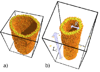
Figure 2: Snapshots of two tether simulations with $20\,000$ lipids and different radii of curvature: a) $\langle R\rangle=24\,\sigma$ b) $\langle R\rangle=12\,\sigma$.

Figure 2 shows two typical snapshots of equilibrated cylindrical vesicles from different simulations. Notice that while fluctuations are clearly visible, they are fairly weak, i. e., the vesicle is to a very good approximation cylindrical. We use the midplane between the two monolayers to denote the average radius $\langle R\rangle$. It is determined by first identifying the axis, next finding the average distance of the second tail bead of the outer leaflet to this axis, $R_{\text{out}}$, and the equivalent for the inner leaflet, $R_{\text{in}}$. We then take $\langle R\rangle=\frac{1}{2}\langle R_{\text{out}}+R_{\text{in}}\rangle$, where the average is taken during long production runs typically extending over 10000-20000 $\tau$. Errors are determined via a blocking analysis. During these runs we also measure the stress tensor $\sigma_{ij}$ using the virial theorem AllenTildesley . Figure 3 shows a typical example of the running average of the three normal stress components. As we observe, the axial stress $\sigma_{zz}$ has a finite value. In contrast, $\sigma_{xx}$ and $\sigma_{yy}$ (as well as all off-diagonal components not shown here) approach zero. This is expected, since no stress is being transported across the $x$- and $y$-direction. The error in $\sigma_{zz}$ is also determined via a blocking analysis.

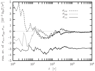
Figure 3: Running average of the diagonal components $\sigma_{xx}$, $\sigma_{yy}$ and $\sigma_{zz}$ of the stress tensor for a cylindrical vesicle with $\langle R\rangle=70\,\sigma$.

One more point concerning the calculation of the stress tensor should be mentioned. In general, deriving accurately the stress (or the pressure) from molecular dynamics simulations is not a trivial aspect. Stress is a collective property with high statistical uncertainty owing to the fluctuations of the instantaneous configurations. In common simulations these fluctuations are very high due to the relatively small size (number of particles) of the systems studied. Therefore large systems and/or long simulation runs are needed. This point is particularly sever in the present case since, as visible in Figure 3, we need to determine very small values of the stress. We have found that, in order to obtain reliable values, the common time step used in coarse grained simulations, $\Delta t=0.01\,\tau$, is too long. With this choice $\sigma_{xx}$ and $\sigma_{yy}$ approached values which were significantly different from zero, a clear sign of a systematic integration error. We thus used the smaller time step $\Delta t=0.005\,\tau$, and for the cases of very small forces, i. e. large $\langle R\rangle$, even a time step of $\Delta t=0.001\,\tau$.

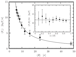
Figure 4: Tensile force $\langle F_{z}\rangle$ as a function of cylinder radius $\langle R\rangle$ for the systems with $N=5000$ lipids (with the exception of the open symbol, which has $N=10\,000$ lipids). The solid line is a fit to Eqn. (7), leading to $\kappa=11.7\,k_{\operatorname{B}}T$. The inset shows the combination $F_{z}R/2\pi$ as a function of rescaled curvature $w/\langle R\rangle$, and the solid line again indicates $\kappa=11.7\,k_{\operatorname{B}}T$.

The tensile force in $z$ direction is obtained from the stress via $F_{z}=\sigma_{zz}L_{x}L_{y}$. Figure 4 shows the force for the systems with $N=5000$ lipids as a function of the average cylinder radius $\langle R\rangle$. As the radius increases, the tensile force $F_{z}$ decreases in accord with Eqn. (7). This is seen even better by looking at the combination $F_{z}R/2\pi$, which is shown in the inset of Fig. 4 as a function of rescaled curvature $w/\langle R\rangle$. Notice that within the error bars of our simulation this expression is perfectly compatible with a constant; a fit gives $\kappa/k_{\operatorname{B}}T=11.7\pm 0.2$, in very good agreement with the value $\kappa/k_{\operatorname{B}}T=12.5\pm 1$ obtained from an analysis of thermal undulation modes (see Fig. 1). A possible quadratic deviation, as suggested by Eqn. (8), can not be identified with any statistical significance. This is all the more amazing when we see that the most strongly curved cylinder has $w/R\approx 0.9$, i. e., a radius of curvature which is only 10% larger than the bilayer thickness $w$! Stated differently, the length $\ell_{4}$ from Eqn. (8) must be a fair bit smaller than $w$. This remarkable robustness of the simple quadratic Helfrich theory down to such small radii of curvature might of course be a special feature of the particular model we have studied, and it would be worthwhile to subject other coarse-grained lipid models to a similar test. But the fact that extremely high curvatures can be imposed without noticing deviations from quadratic continuum theory is in accord with common practice in tether pulling experiments, where the radii of curvature of these membrane tubes are typically in the 10-40 nm range, apparently without ever having triggered the need to include higher order corrections to the elastic behavior Bassereau .

Another practical aspect of our proposed method, is related to numerical efficiency. The traditional method of analyzing the thermal fluctuation spectrum requires very long simulation runs, since ($i$) large systems need to be studied in order to have a series of wave vectors in the regime where continuum methods are applicable, and ($ii$) these long wavelength modes take a particularly long time to equilibrate (the relaxation time of bending modes scales with the fourth power of wavelength). Strictly speaking our method also requires large systems to be studied in order to extrapolate to the zero curvature limit (i. e., $R\rightarrow\infty)$. However, as we have seen in Fig. 4, the asymptotic limit in our case is already reached for fairly small systems which still have a significant curvature. If the same holds for other lipid models – a fact that needs to be checked – their value of $\kappa$ can also be determined via the tether method using fairly small systems and corresponding small simulation times. For example, the point in Figure 4 having $w/\langle R\rangle=0.5$ is taken from a run of only 2-3 days on a single AMD Opteron 2.2GHz processor. For the same system the analysis of the thermal fluctuations needs at least one month on the same machine.

As a final point we would like to address the issue of finite size effects. While the tether force obviously depends on its radius, Eqn. (7) suggests that tether length $L_{z}$ (or equivalently, the number $N$ of lipids) is irrelevant. This is indeed rigorously true in the ground state, but fluctuations might change the picture. We have thus repeated our simulations for systems with a different number of lipids and checked, whether systems with a fixed ratio $L_{z}/N$ (i. e., essentially identical radius) but varying $N$ show any noticeable systematic change in the tensile force $F_{z}$. Figure 5 shows the results of such simulations. As can be seen, the measured forces are, at least within our error bars, compatible with a constant value for a fixed ratio $L_{z}/N$. No finite size effect is detectable. Notice that this also provides another independent check that fluctuations in our system, even though present, are a subdominant effect compared to the main “signal” which is well described by ground state theory.

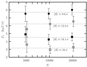
Figure 5: Tensile force $F_{z}$ as a function of system size for systems of different ratio $L_{z}/N$: $\bullet$: 0.01, $\circ$: 0.008, $\blacksquare$: 0.006, $\square$: 0.004. The corresponding average radius $\langle R\rangle$ is als indicated. A slight horizontal offset is included to improve visibility of the error bars.

V Conclusions

We have presented a new method for calculating the bending rigidity of lipid membranes in simulations. It involves the simulation of cylindrical membrane tethers, spanned across the periodic boundary conditions of the simulation box, and measuring their equilibrium radius as well as the tensile force they exercise on the box. In contrast to fluctuation based schemes, which monitor thermally excited shape deformations, our approach actively imposes a deformation on the system and measures the restoring force and is thus not limited to the regime of deformations accessible by thermal energy. In fact, thermal undulations only contribute a small correction to the main observable, in stark contrast to fluctuation schemes in which they provide the dominant signal. For this reason our method is very efficient, also applicable to stiff membranes which show very small undulations to begin with, and does not crucially depend on the relaxation of very slow long wavelength modes. The straightforward access to strong bending permits a check of quadratic continuum theory, without running into difficulties of Monge gauge and its linearization. For the coarse-grained lipid model we explicitly studied we showed continuum theory to be applicable up to curvatures comparable to bilayer thickness. Finite size effects would originate from fluctuations and are thus also weak; in our runs they were not detectable.

We believe that this method provides a powerful alternative to the existing schemes that is worth to be applied to other existing coarse-grained models. Not only is an independent measurement of the elastic modulus very valuable, determining the range of validity of continuum theory for each model would be an important bit of knowledge, given that the curvatures that are regularly imposed in simulations exceed thermally excited ones by at least one or two orders of magnitude.

References

- (1)
- (2) H. Lodish, A. Berk, L. Zirpursky, P. Matsurada, D. Baltimore, and J. Darnell, Molecular Cell Biology, (Freemen and Company, New York, 2000).
- (3) P.B. Canham, J. Theoret. Biol. 26, 61 (1970).
- (4) W. Helfrich, Z. Naturforsch. C 28, 693 (1973).
- (5) E. Evans, Biophys. J. 14, 923 (1974).
- (6) F. Brochard and J.F. Lennon, J. Phys. (Paris) 36, 1035 (1975).
- (7) M.D. Schneider, J.T. Jenkins, and W.W. Webb, J. Phys. (Paris) 45, 1457 (1984).
- (8) J.F. Faucon, M.D. Mitov, P. Meleard, I. Bivas, and P. Bothorel, J. Phys. (Paris) 50, 2389 (1989).
- (9) E. Evans and W. Rawicz, Phys. Rev. Lett. 64, 2094 (1990).
- (10) W. Rawicz, K.C. Olbrich, T. McIntosh, D. Needham, and E. Evans, Biophys. J. 79, 328 (2000).
- (11) J.R. Henriksen and J.H. Ipsen, Eur. Phys. J. E 9, 365 (2002).
- (12) J.R. Henriksen and J.H. Ipsen, Eur. Phys. J. E 14, 149 (2004).
- (13) L. Bo and R.E. Waugh, Biophys. J. 55, 509 (1989).
- (14) J. Dai and M.P. Sheetz, Biophys. J. 68, 988 (1995).
- (15) E. Evans, H. Bownman, A. Leung, D. Needham, and D. Tirrell, Science 273, 933 (1996).
- (16) D. Cuvelier, I. Derenyi, P. Bassereau, and P. Nassoy, Biophys. J. 88, 2714 (2005).
- (17) E. Lindahl and O. Edholm, Biophys. J. 79, 426 (2000).
- (18) S.J. Marrink and A.E. Mark, J. Phys. Chem. B 105, 6122 (2001).
- (19) E.D. Boek, J.T. Padding, W.K. den Otter, and W.J. Briels, J. Phys. Chem. B 109, 19851 (2005).
- (20) R. Goetz, G. Gompper, and R. Lipowsky, Phys. Rev. Lett 82, 221 (1999).
- (21) O. Farago, J. Chem. Phys. 119, 596 (2003).
- (22) M.J. Stevens, J. Chem. Phys. 121, 11942 (2004).
- (23) I.R. Cooke, M. Deserno, and K. Kremer, Phys. Rev. E 72, 011506 (2005).
- (24) I.R. Cooke and M. Deserno, J. Chem. Phys. 123, 224710 (2005).
- (25) G. Brannigan and F.L.H. Brown, Biophys. J. 90, 1501 (2006).
- (26) W.K. den Otter and W.J. Briels, J. Chem. Phys. 118, 4712 (2003).
- (27) O. Farago and P. Pincus, J. Chem. Phys. 120, 2934 (2004).
- (28) J.-B. Fournier and P. Galatola, in preparation.
- (29) R, Capovilla, J. Guven, and J.A. Santiago, J. Phys. A: Math. Gen. 36, 6281 (2003).
- (30) H.J. Limbach, A. Arnold, B.A. Mann, and C. Holm, Comp. Phys. Comm 174, 704 (2006); see also: http://www.espresso.mpg.de/
- (31) G.S. Grest and K. Kremer, Phys. Rev. A 33, 3628 (1986).
- (32) M.P. Allen and D.J. Tildesley, Computer Simulation of Liquids, (Clarendon, Oxford, 1997).