Variable size particle probing of the DLA cluster properties

Abstract

We develop a technique for probing harmonic measure of the diffusion limited aggregation (DLA) cluster surface with the variable size particle and generate one thousand clusters with 50 million particles using original off-lattice killing-free algorithm. Taking, in sequence, the limit of the vanishing size of the probing particles and then sending the growing cluster size to infinity, we achieve the unprecedented accuracy determining the fractal dimension, $D=1.7100(2)$ crucial to characterization of geometric properties of the DLA clusters.

Kinetic interfaces that evolve into two dimensional fractals via the diverse stochastic growth processes are ubiquitous to nature. The systems and physical processes that exhibit kinetic roughening and fractal structure range from firefronts and bacterial colonies to dendrites of various nature, to domain walls in magnets and ferroelectrics, to liquids penetrating porous media, and many others. The study of two-dimensional fractals associated with the kinetic roughening is an exciting and mature branch of statistical physics – see excellent works HHZ ; BH for exhaustive reviews. The generic process governing a good part of these phenomena is the so called two dimensional aggregate growth, which is commonly modeled as the diffusion limited aggregation (DLA) WS and its generalization DBM Pietronero well capturing most of the properties of the random aggregates BH . Past analytical and numerical studies advanced impressively our understanding of DLA (see again HHZ ; BH ), yet there are still several critical issues that remain unresolved, like the controversies related to the multiscale and fractal nature of DLA, to name a few. One of the central questions is the precise value of the DLA fractal dimension $D$, the knowledge of which is crucial for full description of geometric properties and characterization of the DLA clusters. In particular, the exact value of $D$ is necessary for evaluating DLA lacunarity at large growth times.

In the planar, $d{=}2$, geometry the analytical results (see for example Gould ) suggest that the DLA fractal dimension lies in the range $D{=}1.67{-}1.72$; certain rational values like $D{=}5/3$, in Muthu , or $D{=}17/10$, in Hastings were also predicted. On the other hand, Mandelbrot Mandelbrot argued that DLA clusters fill the whole space, i.e. that $D{=}2$. The direct simulations usually produce $D{=}1.715(4)$ for the DLA fractal dimension tm89 ; ms-Os91 ; the simulations DLP based on the conformal mapping HL ; ms-DHOPSS yield $D{=}1.713(5)$.

Conventionally the fractal dimension $D$ is determined from the fit of the growing aggregate (cluster) size, $R$, to the functional dependence

$$R\propto N^{1/D},$$ (1)

where $N$ is the number of particles in the cluster. The cluster size, $R$, can be defined as the radius of the deposition $R_{dep}{=}\langle r_{i}\rangle$, where $r_{i}$ is the position of the $i$-th particle, and brackets stand for the averaging over the ensemble of clusters. The accuracy achieved in the determination of $D$ in the past publications is characterized by the fluctuations RS ; MS ${\cal F}_{D}{=}\left(\langle D^{2}\rangle{-}\langle D\rangle^{2}\right){/}\langle D\rangle^{2}$. The latter decays as ${\cal F}_{D}{\propto}N^{-0.33}{\simeq}N^{-1/3}$ (rather than naively expected ${\propto}1/N\ln N$). As a matter of practice, this implies that in order to achieve the next level of accuracy [one more (forth) digit] one is required to consider clusters with the number of particles exceeding by the factor of 1000 those used in simulations of Refs. tm89 ; ms-Os91 ; DLP . The clusters of such a size, about $N{=}10^{9}$, are not accessible via standard approaches due to the computational speed and computer memory limitations.

In this Letter we develop and report on the alternative approach allowing to reach higher accuracy of the fractal dimension measurement. We exploit the fact that in simulations the diffusing particles always have some finite physical size $\delta$ and that while the true fractal dimension $D$ should not depend on $\delta$, the results of simulations appear to depend on the size of the particles probing harmonic measure. Our idea is to use this dependence in order to parameterize the fractal dimensionality as a function of $\delta$ and, upon finding $D(\delta)$ in a series of numerical experiments, define the fractal dimension  as $D{=}\lim_{\delta{\to}0}D(\delta)$. We will show that our approach allows for a dramatic improvement in the precision in determining $D$.

The accessibility of a particular set of the points at the cluster interface is characterized by the probabilities $p_{k}$ for a particle diffusing from the infinity to hit the cluster at this given subset, $\Gamma_{k}$, of the surface. For the interface of the form of an ideal circle (and the symmetric diffusion), the probabilities are distributed uniformly, and the probability density is just $1/2\pi$ (the harmonic measure). In an irregular cluster most of the probability density is concentrated around the cluster’s tips, whereas the fjords are screened (this effect is often referred to as the “tip effect” and/or the “Faraday screening” Pietronero ; BA ; BB ; HGEH ). The conventional approach to probing the harmonic measure is as follows: (i) The DLA cluster containing $N$ particles is generated; (ii) The positions $r_{i}$ where the next $M$ particles hit the border of the cluster for the first time are stored but the particles do not remain attached to the cluster; (iii) The deposition radius is calculated as

$$R_{dep}(N)\approx\frac{1}{M}\sum_{i=1}^{M}r_{i},$$ (2)

and the sum converges to the integral over harmonic measure $R_{dep}(N){=}{\int}\!dq\,r$ for sufficiently large $M$.

Shown in Figure 1 is the typical variation of $D$ calculated using relation (1) with $R_{dep}$, and representing the half period of oscillations of fractal dimension $D$ with the size of the cluster. The oscillations are related to the spatially nonuniform growth of the cluster: different branches grow with the different speed, and the newborn sub-branches often outgrow the parent branches. The amplitude of the oscillations decrease slowly with the cluster size thus complicating precise determination of the value of $D$.

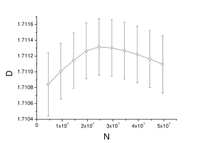
Figure 1: Fractal dimension with error bars as function of the cluster size, computed with $R_{dep}$. Solid line connecting circles is guide for the eye.

Figure 2 shows the part of the cluster branch. The spots where the probe particles hit the surface are marked by the color with the intensity proportional to the logarithm of the particular probability $p_{k}$ for the particle to hit the segment $\Gamma_{k}$. For the sake of better visualization we choose the length of segments equal to the one pixel of the figure. Uncoupled colored segments, $\Gamma_{k}$ (see Fig. 2), constitute only the part of the surface accessible to the diffusing particles. The total length of the accessible cluster interface depends on the size of the probe particles. We choose the probe particle size $\delta$ as a parameter of the particular measurement. The value of $\delta$ controls two processes: (i) the ‘geometrical’ process which is the penetration of the particles inside the fjords where the geometrical bottleneck of the fjords may prevent BB ; HGEH sizable particles to go through, and (ii) the probabilistic process of screening; the latter becomes more effective with the growth of the particle size, $\delta$.

It is important to stress the difference between the measurement of the length of the fractal surface fractal and the measurement of the harmonic measure on the surface within our approach. In the former case, the total length of surface grows with the decreasing scale division value fractal (i.e. the length of the subsets $\Gamma_{k}$ are equal to the ruler size). In the latter case, the probability $p_{k}$ for the particle to hit the subset $\Gamma_{k}$ saturates as $\delta{\to}0$.

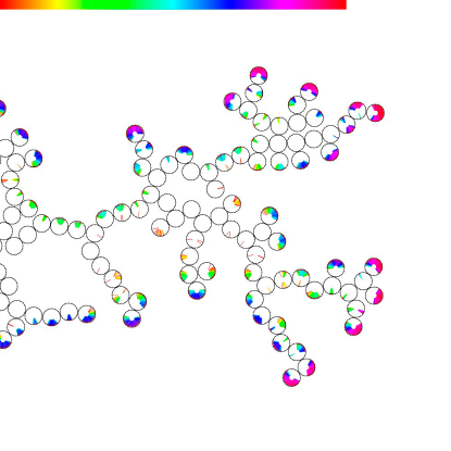
Figure 2: (Color online) Fragment of the cluster with $N{=}10^{4}$ particles and positions of hits by probe particles with radius $\delta{=}1$. Color is proportional to logarithm of the hit probabilities, denoted by the color bar at the top. Probabilities are larger near the tips and smaller inside the fjords.

Shown in Figure 3 is the number of the surface particles having been touched by the probe particles as function of the probing particle size. The solid line is given by the expression $N_{reach}{=}N_{surf}/(1{+}\delta/\delta_{0})^{\alpha}$, with $\alpha{=}0.69(2)$ and $\delta_{0}{=}2.2(1)$. The limit of vanishing size $\delta{\to}0$ gives the limiting number of the reached particles as the total number of surface particles, $N_{surf}{\approx}14,662,525$ (out of total $20$ millions in the cluster).

Figure 3: Number of reachable sites of the cluster as function of the probe particle radius (circles) with the fit described in the text (solid line).

The dependence of $D$ upon $N$ for different $\delta$ is shown in Fig. 4. As we have already mentioned, the dependence on $N$ within the given interval of $N$ and for the fixed $\delta$ is not monotonic for $\delta{<}3$. Thus, we fit results by the formula

$$D(\delta;N)=D(N)+A\delta^{\beta}$$ (3)

and take the limit of $\delta{\to}0$ for the fixed values of the cluster size $N$. The resulting values of $D(N)$ are shown in Fig. 5. Note that now the dependence $D(N)$ has become monotonic. This can be understood as the result of the effective averaging the competition between the growing branches out. We have examined the ensemble of 1000 clusters with 50 million particles for each value of $\delta$. The number of particles $M$ in each event of the measurement necessary to achieve the desired accuracy in $R_{dep}$ of about 0.1%, was typically several tens of thousands. We have found no difference in results when using larger number of probe particles. The error bars represent combined errors from both the ensemble average and the fit. Thus from Fig. 5 one finds at the end of the day the ultimate value of the fractal dimension, $D{=}1.7100(2)$. This is an unprecedented accuracy in the measurements of $D$ exceeding by the order of magnitude the results known from the literature.

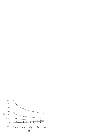
Figure 4: Fractal dimension (symbols) as function of $N$ for $\delta=$0.1, 0.3, 1, 3, 10, 30, 100 from bottom to top. Solid lines connecting circles is guide for the eye.

Figure 5: Fractal dimension as function of $N$ for the limiting value of $\delta=0$. It reach value $D=1.7100(2)$ (plotted with the dotted line) in the limit of large cluster size $N$.

It is instructive to use the same ensemble of clusters in order to evaluate the fractal dimension via the traditional approach introducing the deposition radius as $R_{dep}{=}\langle r\rangle$, the mean square displacement $R_{2}{=}\sqrt{\langle r^{2}\rangle}$, and the radius of gyration $R_{g}{=}\sqrt{\frac{1}{N}\sum_{i{=}1}^{N}\langle r^{2}\rangle}$. The results of the fit to the form (1), where $R$ stands for one of the above radii, are presented in Table 1. Note, that all the obtained values of $D$ are larger than that of $D{=}1.7100(2)$ derived by the method of present work.

Since DLA clusters grow randomly, a center of the cluster mass $R_{M}{=}\sqrt{\frac{1}{N}\left|\sum_{i{=}1}^{N}r_{i}\right|}$ performs random walks in the plane. Accordingly, the distance from the original position of a seed particle to the center of mass grows as $\sqrt{N}$ and the number of particles is proportional to the time of the random walk . The average value of $R_{M}$ for $N{=}5{\cdot}10^{7}$ is $\langle R_{M}\rangle{\approx}1000$ which should be compared to $\langle R_{g}\rangle{\approx}30000$ and the penetration depth $\xi{\approx}7000$. The average angular position of the center of mass (averaged over an ensemble) is also a stochastic function of time, although at each realization of the cluster angular correlations are observed (some of the branches grow faster within a given time interval MSV-long ).

The important question now is whether the choice of the coordinate frame influences the final result and the value of the fractal dimensionality. Indeed, when determining $D$ one can choose the origin at either (i) the position of the seed particle, or (ii) at the (evolving with time) position of the center of gravity, or else (iii) at the ’center of the charge gravity’ (the latter is most appropriate for the DMB case). We have performed averaging according to Eq. (2) finding $D$ from the fit to $\tilde{R}_{dep}$, $\tilde{R}_{2}$, and $\tilde{R}_{g}$, placing the origin of the reference frame to the seed particle (left column of the Table 1) and to the center of gravity (right column). One sees that for all the quantities the choice of the reference frame is irrelevant (within the accuracy of the computation), although the ensemble of clusters should be large enough to insure this convergence.

	$r$ to seed	$r$ to center-of-mass
$R_{dep}$	1.7098(12)	1.7111(6)
$R_{2}$	1.71155(56)	1.71149(54)
$R_{g}$	1.71149(30)	1.71133(30)

Table 1: Fractal dimension estimated by the standard method using the reference frames centered at the seed particle (left column) and at the center of gravity (right column) respectively.

In conclusion, we have developed a technique for the high precision analysis of the geometrical properties of DLA clusters, in particular the evaluation of its lacunarity in the long time limit. Our approach offers a perfect tool for further advance in our understanding of the fjord screening behavior. In particular, the long standing problems of the behavior of the $p_{min}$, which is the minimal growth probability (in DBM language) or probability to hit given segment of the cluster surface (in DLA language) can be efficiently addressed via the developed approach. The behavior of the latter probability is related to the phase transition in the multifractal spectrum LS . To the best of our knowledge, this probability was estimated only within the “tunnel configuration” BA technique and had never been measured in the simulations of the “typical configuration” LAS .

We are pleased to thank S. Korshunov for important and enlightening discussions. This work is supported by the US DOE Office of Science under contract No. W31-109-ENG-38 and by the Russian Foundation for Basic Research.

References

- (1)
- (2) T. Halpin-Healy and Y.C. Zhang, Physics Reports 254, 215 (1995)
- (3) A. Bunde and S. Havlin, eds., Fractals and Disordered Systems (Springer, Berlin, 1996).
- (4) T.A. Witten and L.M. Sander, Phys. Rev. Lett. 47, 1400 (1981).
- (5) L. Niemeyer, L. Pietronero, H.J. Wiesmann, Phys. Rev. Lett., 52, 1033 (1984).
- (6) H. Gould, F. Family, and H.E. Stanley, Phys. Rev. Lett. 50, 686 (1983).
- (7) M. Muthukumar, Phys. Rev. Lett. 50, 839 (1983).
- (8) M.B. Hastings, Phys. Rev. E 55, 135 (1997).
- (9) B. Mandelbrot, Physica A 191, 95 (1992).
- (10) S. Tolman and P. Meakin, Physica A 158, 801 (1989); Phys. Rev. A 40, 428 (1989).
- (11) P. Ossadnik, Physica A 176 (1991) 454, ibid. 195, 319 (1993).
- (12) B. Davidovitch, A. Levermann, and I. Procaccia, Phys. Rev. E 62, R5919 (2000).
- (13) M.B. Hastings and L.S. Levitov, Physica D 116, 244 (1998).
- (14) B. Davidovitch, H.G.E. Hentschel, Z. Olami, I. Procaccia, L.M. Sander, and E. Somfai, Phys. Rev. E 59, 1368 (1999).
- (15) T.A. Rostunov, L.N. Shchur, JETP 95, 145 (2002)
- (16) A. Yu. Menshutin, L. N. Shchur, Phys. Rev. E 73, 011407 (2006).
- (17) R. Blumenfeld, A. Aharony, Phys. Rev. Lett. 62, 2977 (1989)
- (18) R.C. Ball, R. Blumenfeld, Phys. Rev. A 44, R828 (1991).
- (19) H.G.E. Hentschel, Phys. Rev. A 46, R7379 (1992).
- (20) B.B. Mandelbrot, Science 155, 636 (1967).
- (21) A.Yu. Menshutin, L.N. Shchur, and V.M. Vinokur, unpublished.
- (22) J. Lee, H.E. Stanley, Phys. Rev. Lett. 61, 2945 (1988)
- (23) J. Lee, P. Alström, and H.E. Stanley, Phys. Rev. Lett. 62, 3013 (1989)