Quasiparticle self-consistent $GW$ method; a basis for the independent-particle approximation

Abstract

We have developed a new type of self-consistent scheme within the $GW$ approximation, which we call quasiparticle self-consistent $GW$ (QS$GW$). We have shown that QS$GW$describes energy bands for a wide-range of materials rather well, including many where the local-density approximation fails. QS$GW$ contains physical effects found in other theories such as LDA$+U$, SIC and $GW$ in a satisfactory manner without many of their drawbacks (partitioning of itinerant and localized electrons, adjustable parameters, ambiguities in double-counting, etc.). We present some theoretical discussion concerning the formulation of QS$GW$, including a prescription for calculating the total energy. We also address several key methodological points needed for implementation. We then show convergence checks and some representative results in a variety of materials.

In the 1980’s, algorithmic developments and faster computers made it possible to apply Hedin’s $GW$ approximation ($GW$​A) Hedin (1965) to real materials Strinati et al. (1980); Pickett and Wang (1984). Especially, Hybertsen and Louie Hybertsen and Louie (1986) first implemented the $GW$​A within an ab-initio framework in a satisfactory manner. Theirs was a perturbation treatment starting from the Kohn-Sham eigenfunctions and eigenvalues given in the local density approximation (LDA) to density functional theory (DFT)Hohenberg and Kohn (1964); Kohn and Sham (1965). We will denote this approach here as 1shot-$GW$. Until now 1shot-$GW$ has been applied to variety of materials, usually in conjunction with the pseudopotential (PP) approximation. Quasiparticle (QP) energies so obtained are in significantly better agreement with experiments than the LDA Kohn-Sham eigenvaluesAryasetiawan and Gunnarsson (1998).

However, we have recently shown that 1shot-$GW$ has many significant failings. Even in simple semiconductors it systematically underestimates optical gapsKotani and van Schilfgaarde (2002); Usuda et al. (2004); Fleszar and Hanke (2005); van Schilfgaarde et al. . In general, the quality of results are closely tied to the quality of the LDA starting point. For more complicated cases where the LDA eigenfunctions are poor, 1shot-$GW$ can fail even qualitativelyvan Schilfgaarde et al. .

A possible way to overcome this difficulty is to determine the starting point self-consistently. The effects of the eigenvalue-only self-consistency (keeping the eigenfunctions as given in LDA), was discussed by Surh, Louie, and CohenSurh et al. (1991). Recently, Luo, Ismail-Beigi, Cohen, and Louie Luo et al. (2002) applied it to ZnS and ZnSe, where they showed that the band gaps of 1shot-$GW$ 3.19 eV and 2.32 eV for ZnS and ZnSe are increased to 3.64 eV and 2.41 eV by the eigenvalue-only self-consistency (see Table 4 also). The differences suggest the importance of this self-consistency. Furthermore, for ZnSe, the value 2.41 eV changes to 2.69 eV when they use eigenfunctions given by generalized gradient approximation (GGA). This difference suggests that we may need to look for a means to determine optimum eigenfunctions for $GW$A. Aryasetiawan and Gunnarsson applied another kind of self-consistent scheme to NiO Aryasetiawan and Gunnarsson (1995). They introduced a parameter for the non-local potential which affects the unoccupied $e_{g}$ level, and made it self-consistent. They showed that the band gap of 1shot-$GW$ is $\sim$1 eV, and that it is improved to $\sim$5.5 eV by the self-consistency.

Based on these self-consistency ideas, we have developed a new ab-initio approach to $GW$ Faleev et al. (2004); van Schilfgaarde et al. (2006); Chantis et al. (2006a, b), which we now call “quasiparticle self-consistent $GW$” (QSGW) method. QSGW is a first-principles method that stays within the framework of Hedin’s $GW$​A, that is, QSGW is a perturbation theory built around some noninteracting Hamiltonian. It does not depend on the LDA anymore but rather determines the optimum noninteracting Hamiltonian in a self-consistent manner. We have shown that QSGW satisfactorily describes QP energies for a wide range of materials. Bruneval, Vast and Reining Bruneval et al. (2006a) implemented it in the pseudopotential scheme, and gave some kinds of analysis including the comparison with the Hartree-Fock method and with the Coulomb-hole and Screened exchange (COHSEX) methods.

The present paper begins with a derivation of the fundamental equation of QSGW, and some theoretical discussion concerning it (Sec. I). The fundamental equation is derived from the idea of a self-consistent perturbation. We also present a means for computing the total energy through the adiabatic connection formalism. Next, we detail a number of key methodological points (Sec. II). The present implementation is unique in that it makes no pseudopotential or shape approximation to the potential, and it uses a mixed basis for the response function, Coulomb interaction, and self-energy, which enables us to properly treat core states. The $GW$A methodology is presented along with some additional points particular to self-consistency. In Sec. III, we show some convergence checks, using GaAs as a representative system. Then we show how QSGW works by comparing it to other kinds of $GW$​A for compounds representative of different materials classes: semiconductors C, Si, SiC, GaAs, ZnS, and ZnSe; oxide semiconductors ZnO and Cu₂O; transition metal monoxides MnO and NiO; transition metals Fe and Ni.

I Theory

I.1 $GW$​A

Let us summarize the $GW$​A Hedin (1965); Hybertsen and Louie (1986) for later discussion. Here we omit spin index for simplicity. Generally speaking, we can perform $GW$A from some given one-body Hamiltonian $H^{0}$ written as

$$H^{0}=\frac{-\nabla^{2}}{2m}+V^{\rm eff}({\bf r},{\bf r}^{\prime}).$$ (1)

The one-particle effective potential $V^{\rm eff}({\bf r},{\bf r}^{\prime})$ can be non-local, though it is local, i.e. $V^{\rm eff}({\bf r},{\bf r}^{\prime})=V^{\rm eff}({\bf r})\delta({\bf r}-{\bf r}^{\prime})$ when generated by the usual Kohn-Sham construction. $H^{0}$ determines the set of eigenvalues $\{\varepsilon_{i}\}$ and eigenfunctions $\{\Psi_{i}({\bf r})\}$. From them we can construct the non-interacting Green’s function $G^{0}$ as

$$G^{0}\left({\bf r},{\bf r}^{\prime},\omega\right)=\sum\limits_{i}{\frac{\Psi_{i}({\bf r})\Psi_{i}^{*}({\bf r}^{\prime})}{{\omega-\varepsilon_{i}\pm i\delta}}},$$ (2)

where $-i\delta$ is for occupied states, and $+i\delta$ for unoccupied states. Within the RPA (random-phase approximation), the screened Coulomb interaction is

$$W=\epsilon^{-1}v=\left(1-v\Pi\right)^{-1}v$$ (3)

where $\Pi=-iG^{0}\times{}G^{0}$ is the proper polarization function, and $v({\bf r},{\bf r}^{\prime})=\frac{e^{2}}{|{\bf r}-{\bf r}^{\prime}|}$ is the bare Coulomb interaction. $\epsilon$ denotes the dielectric function. As seen in e.g., works by Alouani and co-workers Alouani and Wills (1996); Arnaud and Alouani (2001), $W$ calculated from a reasonable $H^{0}$ should be in good agreement with experiments, even if $W$ does not satisfy the $f$-sum rule because $H^{0}$ is non-local Alouani and Wills (1996) (because of the so-called scissors operator).

Hedin’s $GW$​A gives the self-energy $\Sigma({\bf r},{\bf r}^{\prime}\!\!,\omega)$ as

$$\Sigma({\bf r},{\bf r}^{\prime}\!\!,\omega)\!=\!\frac{i}{2\pi}\!\!\int\!\!d\omega^{\prime}G^{0}({\bf r},{\bf r}^{\prime}\!\!,\omega-\omega^{\prime})W({\bf r},{\bf r}^{\prime}\!\!,\omega^{\prime})e^{-i\delta\omega^{\prime}}\!\!.$$ (4)

From this self-energy, the external potential $V^{\rm ext}$ from the nuclei, and the Hartree potential $V^{\rm H}$ which is calculated from the electron density through $G^{0}$, we obtain an $\omega$-dependent one-body effective potential $V^{GW}(\omega)$ :

$$V^{GW}(\omega)=V^{\rm ext}+V^{\rm H}+\Sigma(\omega).$$ (5)

Note that $V^{\rm H}$ is detemined from the density which is calculated for the non-interacting system specified by $H^{0}$. For simplicity we omit arguments $({\bf r},{\bf r}^{\prime})$. Then the one-body Green function is given as $G=1/({-\nabla^{2}}{2m}+V^{GW}(\omega))$. $V^{\rm ext}$ and $V^{\rm H}$ are local and $\omega$-independent potentials. Thus the $GW$​A maps $V^{\rm eff}$ to $V^{GW}(\omega)$. In other words, the $GW$​A generates a perturbative correction ${\it\Delta}V(\omega)$ to the one-particle potential $V^{\rm eff}$, written as

$${\it\Delta}V(\omega)=V^{GW}(\omega)-V^{\rm eff}.$$ (6)

$V^{GW}(\omega)$ and ${\it\Delta}V(\omega)$ can be regarded as functionals of $V^{\rm eff}$ (or $H^{0}$).

In the standard 1shot-$GW$ with $H^{0}$ generated by the LDA, $V^{\rm eff}$ is the LDA Kohn-Sham Hamiltonian. Neglecting off-diagonal terms, the QP energy (QPE) is

$${E_{{\bf k}n}}={\varepsilon_{{\bf k}n}}+Z_{{\bf k}n}[\langle{\Psi_{{\bf k}n}}|\Sigma({\bf r},{\bf r}^{\prime},{\varepsilon_{{\bf k}n}})|{\Psi_{{\bf k}n}}\rangle-\langle{\Psi_{{\bf k}n}}|V_{\rm xc}^{\rm{LDA}}({\bf r})|{\Psi_{{\bf k}n}}\rangle],$$ (7)

where $Z_{{{\bf k}}n}$ is the QP renormalization factor:

$$Z_{{\bf k}n}=\left[1-\langle{\Psi_{{\bf k}n}}|\frac{\partial}{\partial\omega}\Sigma({\bf r},{\bf r}^{\prime},{\varepsilon_{{\bf k}n}})|{\Psi_{{\bf k}n}}\rangle\right]^{-1}.$$ (8)

Subscripts label the wave vector ${\bf k}$ and band index $n$. We will write them later as a compound index, $i\equiv({\bf k},n)$. Eq. (7) is the customary way QPEs are calculated in $GW$. However, as we discussed in Ref. van Schilfgaarde et al. , using $Z$=1 instead of Eq. (8) is usually a better approximation; see also Sec. III. Chapter 7 of Ref.Mahan (1990) presents another analysis where $Z$=1 is shown to be a better approximation, in the context of the Frölich Hamiltonian. In any case, we have to calculate matrix elements $\langle{\Psi_{{\bf k}n^{\prime}}}|\Sigma({\bf r},{\bf r}^{\prime},\omega)|{\Psi_{{\bf k}n}}\rangle$ as accurately and as efficiently as possible (off-diagonal elements are necessary in the QSGW case, as explained below).

As we showed in Ref. van Schilfgaarde et al. , $H^{0}$ generated by LDA is not necessarily a good approximation. [Even the $H^{0}$ for “true Kohn-Sham” Hamiltonian in DFT can be a poor descriptor of QP excitation energies Kotani (1998).] For example, time-reversal symmetry is automatically enforced because $V^{\rm eff}$ is local (and thus real). This symmetry is strongly violated in open $f$-shell systems Chantis et al. (2006b). The bandgap of a relatively simple III-V semiconductor, InN, is close to zero Kotani and van Schilfgaarde (2002); Usuda et al. (2004); also the QP spectrum of NiO is little improved over LDA Faleev et al. (2004). A variety of other examples could be cited where $GW$A starting from $H^{0}=H^{\rm{LDA}}$ is a poor approximation. (In contrast, see Sec. III and Ref. van Schilfgaarde et al. (2006) to see how QSGW gives consistently good agreement with experiment.)

I.2 Quasiparticle self-consistent $GW$

QSGW is a formalism which determines $V^{\rm eff}$ (or $H^{0}$) self-consistently within the $GW$A, without depending on LDA or DFT. If we have a mapping procedure $V^{GW}(\omega)\rightarrow V^{\rm eff}$, we can close the equation to determine $V^{\rm eff}$, i.e. determine $V^{\rm eff}$ self-consistently by $V^{\rm eff}\rightarrow V^{GW}(\omega)\rightarrow V^{\rm eff}\rightarrow\dots$. The main idea to determine the mapping is grounded in the concept of the QP. Roughly speaking, $V^{\rm eff}$ is determined so as to reproduce the QP generated from $V^{GW}(\omega)$. In the following, we explain how to determine this $V^{GW}(\omega)\rightarrow V^{\rm eff}$, and derive the fundamental QSGW equation Faleev et al. (2004); van Schilfgaarde et al. (2006); Chantis et al. (2006a, b).

Based on Landau’s QP picture, there are fundamental one-particle-like excitations denoted as quasiparticles (QP), at least around the Fermi energy $E_{\rm F}$. The QPEs and QP eigenfunctions (QPeigs), $\{E_{i},\Phi_{i}({\bf r})\}$, are given as Hedin (1965)

$$\left[\frac{-\nabla^{2}}{2m}+V^{\rm ext}+V^{\rm H}+{\rm Re}[\Sigma(E_{i})]-E_{i}\right]|\Phi_{i}\rangle=0.$$ (9)

We refer to the states characterized by these $E_{i}$ and $\Phi_{i}({\bf r})$ as the dressed QP. Here ${\rm Re}[X]$ means just take the hermitian part of $X$ so $E_{i}$ is real for $E_{i}$. This is irrelevant around $E_{\rm F}$ because the anti-hermitian part of $\Sigma(E_{i})$ goes to zero as $E_{i}\to$ $E_{\rm F}$. On the other hand, we have another one-particle picture described by $H^{0}$; we name these QPs as bare QPs, and refer to the QPEs and eigenfunctions corresponding to $H^{0}$ as $\{\varepsilon_{i},\Psi_{i}({\bf r})\}$.

Let us consider the difference and the relation of these two kinds of QP. The bare QP is essentially consistent with the Landau-Silin QP picture, discussed by, e.g., Pines and Nozieres in Sec. 3.3, Ref. Pines and Nozieres (1966). The bare QP interact with each other via the bare Coulomb interaction. The bare QP given by ${H^{0}}$ evolve into the dressed QP when the interaction $\hat{H}-\hat{H^{0}}$ is turned on adiabatically. Here $\hat{H}$ is the total Hamiltonian (See Eq. (12)); and the hat signifies that $\hat{H}$ is written in second quantized form. $\hat{H^{0}}$ and $H^{0}$ are equivalent. The dressed QP consists of the central bare QP and an induced polarization cloud consisting of other bare QP ; this view is compatible with the way interactions are treated in the $GW$​A.

$H^{0}$ generating the bare QPs represents a virtual reference system just for theoretical convenience. There is an ambiguity in how to determine $H^{0}$; in principle, any $H^{0}$ can be used if $\hat{H}-\hat{H^{0}}$ could be completely included. However, as we evaluate the difference $\hat{H}-\hat{H^{0}}$ in some perturbation method like $GW$A, we must utilize some optimum (or best) $\hat{H^{0}}$: $\hat{H^{0}}$ should be chosen so that the perturbative contribution is as small as possible. A key point remains in how to define a measure of the size of the perturbation. We can classify our QSGW method as a self-consistent perturbation method which self-consistently determines the optinum division of $\hat{H}$ into the main part $H^{0}$ and the residual part $\hat{H}-\hat{H^{0}}$. There are various possible choices for the measure; however, here we take a simple way, by requiring that the two kinds of QPs discussed in the previous paragraphs correspond as closely as possible. We choose $H^{0}$ so as to repoduce the dressed QPs. In other words, we assign the difference of the QPeig (and also the QPE) between the bare QP and the dressed QP as the measure, and then we minimize it. From the physical point of view, this means that the motion of the central electron of the dressed QP is not changed by $\hat{H}-\hat{H^{0}}$. Note that $\hat{H}-\hat{H^{0}}$ contains two kinds of contributions: not only the Coulomb interaction but also the one-body term $V^{\rm ext}-V^{\rm eff}$. The latter gives a counter contribution that cancel changes caused by the Coulomb interaction.

We now explain how to obtain an expression in practice. Suppose that self-consistency has been somehow attained. Then we have $\{\varepsilon_{i},\Psi_{i}\}\approx\{E_{i},\Phi_{i}\}$ around $E_{\rm F}$. $\{\Psi_{i}\}$ is a complete set because they come from some $H^{0}$, though the $\{\Phi_{i}\}$ are not. Then we can expand ${\rm Re}[\Sigma(e_{i})]|\Psi_{i}\rangle$ ($\approx{\rm Re}[\Sigma(E_{i})]|\Phi_{i}\rangle$) in $\{\varepsilon_{i},\Psi_{i}\}$ as

$${\rm Re}[\Sigma(\varepsilon_{i})]|\Psi_{i}\rangle=\sum_{j,i}|\Psi_{j}\rangle{\rm Re}[\Sigma(\varepsilon_{i})]_{ji},$$

where ${\rm Re}[\Sigma(\omega)]_{ij}=\langle\Psi_{i}|{\rm Re}[\Sigma(\omega)]|\Psi_{j}\rangle$. Then we introduce an energy-independent operator ${R}$ defined as

$${R}=\sum_{j,i}|\Psi_{j}\rangle{\rm Re}[\Sigma(\varepsilon_{i})]_{ji}\langle\Psi_{i}|,$$

which satisfies ${R}|\Psi_{i}\rangle={\rm Re}[\Sigma(\varepsilon_{i})]|\Psi_{i}\rangle$. Thus we can use this ${R}$ instead of ${\rm Re}[\Sigma(E_{i})]$ in Eq. (9); however, ${R}$ is not hermitian thus we take only the hermitian part of ${R}$ as $V^{\rm xc}={\rm Re}[{R}]$;

$$V^{\rm xc}=\frac{1}{2}\sum_{ij}|\Psi_{i}\rangle\left\{{{\rm Re}[\Sigma(\varepsilon_{i})]_{ij}+{\rm Re}[\Sigma(\varepsilon_{j})]_{ij}}\right\}\langle\Psi_{j}|,\ \ \ \ {\rm mode\!-\!A}$$ (10)

for the calculation of $\{E_{i},\Phi_{i}\}$ ($\approx\{\varepsilon_{i},\Psi_{i}\}$) in Eq. (9). Thus we have obtained a mapping $V^{\rm eff}\rightarrow V^{GW}(\omega)\rightarrow V^{\rm eff}$: for given $V^{\rm eff}$ we can calculate $V^{\rm xc}$ in Eq. (10) through $\Sigma(\omega)$ in the $GW$A. With this $V^{\rm xc}$ together with $V^{\rm H}$, which is calculated from the density for $G^{0}$ (or $H^{0}$), we have a new $V^{\rm eff}$. The QSGW cycle determines all $H^{0},V^{\rm eff}$, $W$ and $G$ self-consistently. As shown in Sec. III and also in Refs.Faleev et al. (2004); van Schilfgaarde et al. (2006); Chantis et al. (2006a), QSGW systematically overestimates semiconductor band gaps a little, while the dielectric constant $\epsilon_{\infty}$ is slightly too small van Schilfgaarde et al. (2006).

It is possible to derive Eq. (10) in a straightforward manner from a norm-functional formalism. We first define a positive-definite norm functional $M(V^{\rm eff})={\rm Tr}[{\rm Re}[{\it\Delta}V(\omega)]\rho{\rm Re}[{\it\Delta}V(\omega)]]$ to measure the size of pertubative contribution. Here the weight function $\rho=\delta(\omega-H^{0})$ defines the measure; ${\rm Tr}$ is for space, spin and $\omega$. For fixed $\rho$, this $M(V^{\rm eff})$ is treated as a functional of $V^{\rm eff}$ because $V^{\rm eff}$ determines ${\it\Delta}V(\omega)$ through Eq. (6) in the $GW$A. As $M(V^{\rm eff})=\sum_{j,i}|\langle\Psi_{i}|{\rm Re}[V^{GW}(\varepsilon_{j})]-V^{\rm eff}|\Psi_{j}\rangle|^{2}$, we can show its minimum occurs when Eq. (10) is satisfied in a straightforward manner. This minimization formalism clearly shows that QSGW determines $V^{\rm eff}$ for a given $V^{\rm ext}$; in addition, it will be useful for formal discussions of conservation laws and so on. The discussion in this paragraph is similar to that given in Ref. van Schilfgaarde et al., 2006, though we use a slightly different $M(V^{\rm eff})$.

Eq. (10) is derived from the requirement so that $\{\varepsilon_{i},\Psi_{i}\}\approx\{E_{i},\Phi_{i}\}$ around $E_{\rm F}$. This condition does not necessarily determine $V^{\rm xc}$ uniquely. It is instructive to evaluate how results change when alternative ways are used to determine $V^{\rm eff}$. In Ref. Faleev et al. (2004) we tested the following:

$$V^{\rm xc}=\sum_{i}|\psi_{i}\rangle{\rm Re}[\Sigma(\varepsilon_{i})]_{ii}\langle\psi_{i}|,+\sum_{i\neq j}|\psi_{i}\rangle{\rm Re}[\Sigma(\mbox{$E_{\rm F}$})]_{ij}\langle\psi_{j}|,\ \ \ \ {\rm mode\!-\!B}$$ (11)

In this form (which we denote as ‘mode-B’), the off-diagonal elements are evaluated at $E_{\rm F}$. The diagonal parts of Eq. (11) and Eq. (10) are the same. As noted in Ref. Faleev et al. (2004), and as discussed in Sec. III, Eqs. (10) and (11) yield rather similar results, though we have found that mode-A results compare to experiment in the most systematic way.

As the self-consistency through Eq. (10) (or Eq. (11)) results in $\{\varepsilon_{i},\Psi_{i}\}\approx\{E_{i},\Phi_{i}\}$, we can attribute physical meaning to bare QP: we can use the bare QP in the independent-particle approximation Ashcroft and Mermin (1976), when, for example, modeling transport within the Boltzmann-equation Fischetti and Laux (1988). It will be possible to calculate scattering rates between bare QP given by $H^{0}$, through calculation of various matrix elements (electron-electron, electron-phonon, and so on). The adiabatic connection path from $\hat{H^{0}}$ to $\hat{H}$ used in QSGW is better than the path in the Kohn-Sham theory where the eigenfunction of $H_{\rm KS}$ (Kohn-Sham Hamiltonian) evolves into the dressed QP. Physical quantities along the path starting from $H_{\rm KS}$ may not be very stable. For example, the band gap can change very much along the path (it can change from metal to insulator in some cases, e.g. in Ge and InN van Schilfgaarde et al. ; QSGW is free from this problem van Schilfgaarde et al. (2006)), even if it keeps the density along the path. [Note: Pines and Nozieres (Ref. Pines and Nozieres (1966), Sec. 1.6) use the terms ‘bare QP’ and ‘dressed QP’ differently than what is meant here. They refer to eigenstates of $\hat{H}$ as ‘bare QP,’ and spatially localized QP as ‘dressed QP’ in the neutral Fermi liquid.]

From a theoretical point of view, the fully sc $GW$ Schöne and Eguiluz (1998); Ku and Eguiluz (2002) looks reasonable because it is derived from the Luttinger-Ward functional $E[G]$. This apparently keeps the symmetry of $G$, that is, $E[G]=E[{\cal R}[G]]$ where ${\cal R}[G]$ denotes some $G\to G$ mapping (any symmetry in Hamiltonian, e.g. time translation and gauge transformation); this clearly results in the conservation laws for external perturbations Baym and Kadanoff (1961) because of Noether’s theorem (exactly speaking, we need to start from the effective action formalism for the dynamics of $G$ Fukuda et al. (1994)). However, it contains serious problems in practice. For example, fully sc $GW$ uses $W$ from $\Pi=-iG\times G$; this includes electron-hole excitations in its intermediate states with the weight of the product of renormalization factors $Z\times Z$. This is inconsistent with the expectation of the Landau-Silin QP picture Faleev et al. (2004); Bechstedt et al. (1997). In fact, as we discuss in Appendix A, the effects of $Z$ factor included in $G$ are well canceled because of the contribution from the vertex; Bechstedt et al. showed the $Z$-factor cancellation by a practical calculation at the lowest order Bechstedt et al. (1997). In principle, such a deficiency should be recovered by the inclusion of the contribution from the vertex; however, we expect that such expansion series should be not efficient.

Generally speaking, perturbation theories in the dressed Green’s function $G$ (as in Luttinger-Ward functional) can be very problematic because $G$ contains two different kinds of physical quantities to intermediate states: the QP part (suppressed by the factor $Z$) and the incoherent part (e.g. plasmon-related satellites). Including the sum of ladder diagrams into $\Pi$ via the Bethe-Salpeter equation, should be a poorer approximation if $G$ is used instead of $G^{0}$, because the one-particle part is suppressed by $Z$ factors; also the contribution from the incoherent part can give physically unclear contributions. The same can be said about the $T$-matrix treatment Springer et al. (1998). Such methods have clear physical interpretation in a QP framework, i.e. when the expansion is through $G^{0}$. A similar problem is encountered in theories such as “dynamical mean field theory”+$GW$ Biermann et al. (2003), where the local part of the proper polarization function is replaced with a “better” function which is obtained with the Anderson impurity model. This question, whether the perturbation should be based on $G$, or on $G^{0}$, also appeared when Hedin obtained an equation to determine the Landau QP parameters; See Eq. (26.12) in Ref. Hedin (1965).

As we will show in Sec. III (see Ref. van Schilfgaarde et al. (2006) also), QSGW systematically overestimates band gaps, consistent with systematic underestimation of $\epsilon_{\infty}$. This looks reasonable because $W$ does not include the electron-hole correlation within the RPA. Its inclusion would effectively reduce the pair excitation energy in its intermediate states. If we do include such kind of correlation for $W$ at the level of the Bethe-Salpeter equation, we will have an improved version of QSGW. However, the QPE obtained from $G^{0}W$ with such a $W$ corresponds to the $\Gamma=1$ approximation, from the perspective of the $\Sigma=G^{0}W\Gamma$ approximation, as used by Mahan and Sernelius Mahan and Sernelius (1989); the contribution from $\Gamma$ is neglected. In order to include the contribution properly, we need to use the self-energy derived from the functional derivative of $E_{c}$ as shown in Eq. (21) in next section, where we need to include the proper polarization $\Pi_{\lambda}$ which includes such Bethe-Salpeter contributions; then we can include the corresponging $\Gamma$. It looks complicated, but it will be relatively easy to evaluate just the shift of QPE with neglecting the change of QPeig; we just have to evaluate the change of $E_{c}$ numerically, when we add (or remove) an electron to $G_{0}$. However, numerical evalution for these contributions are demanding, and beyond the scope of this paper.

I.3 Total energy

Once $V^{\rm eff}$ is given, we can calculate the total energy based on the adiabatic connection formalism Fuchs and Gonze (2002); Miyake et al. (2002); Kotani (1998); Fukuda et al. (1994). Let us imagine an adiabatic connection path where the one-body Hamiltonian $H^{0}=\frac{-\nabla^{2}}{2m}+V^{\rm eff}$ evolves into the total Hamiltonian $\hat{H}$, which is written as

$$\hat{H}=\hat{H}^{\rm k}+\hat{V}^{\rm ee}+\hat{V}^{\rm ext},$$ (12)

$$\hat{H}^{\rm k}=\sum_{\sigma}\int d{\bf r}\hat{\psi}^{\dagger}_{\sigma}({\bf r})(-\frac{\nabla^{2}}{2m})\hat{\psi}_{\sigma}({\bf r}),$$ (13)

$$\hat{V}^{\rm ext}\!=\!\sum_{\sigma}\int d{\bf r}V^{\rm ext}_{\sigma}({\bf r})\hat{n}_{\sigma}({\bf r}),$$ (14)

$$\hat{V}^{\rm ee}\!=\!\frac{1}{2}\sum_{\sigma\sigma^{\prime}}\int\!\!d{\bf r}d{\bf r}^{\prime}v({\bf r},{\bf r}^{\prime})\times$$

$${\hat{\psi}^{\dagger}_{\sigma}({\bf r})\hat{\psi}^{\dagger}_{\sigma^{\prime}}({\bf r}^{\prime})\hat{\psi}_{\sigma^{\prime}}({\bf r}^{\prime})\hat{\psi}_{\sigma}({\bf r})}.$$ (15)

$\hat{V}^{\rm eff}$ is also defined with $V^{\rm eff}$ instead of $V^{\rm ext}$ in Eq. (14). We use standard notation for the field operators $\hat{\psi}_{\sigma}({\bf r})$, spin index $\sigma$, and external potential $V^{\rm ext}_{\sigma}({\bf r})$. We omit spin indexes below for simplicity.

A path of adiabatic connection can be parametrized by $\lambda$ as $\hat{H}^{\lambda}=\hat{H}^{0}+\lambda(\hat{V}^{\rm ext}-\hat{V}^{\rm eff}+\hat{V}^{\rm ee})$. Then the total energy $E$ is written as

$$E=E^{0}+\int_{0}^{1}d\lambda\frac{dE^{\lambda}}{d\lambda}=E^{0}+\int_{0}^{1}d\lambda\langle 0_{\lambda}|\hat{V}^{\rm ext}-\hat{V}^{\rm eff}|0_{\lambda}\rangle+\int_{0}^{1}d\lambda\langle 0_{\lambda}|\hat{V}^{\rm ee}|0_{\lambda}\rangle,$$ (16)

where $|0_{\lambda}\rangle$ is the ground state for $\hat{H}^{\lambda}$. We define $E^{\rm ext}=\int_{0}^{1}d\lambda\langle 0_{\lambda}|\hat{V}^{\rm ext}|0_{\lambda}\rangle$. This path is different from the path used in DFT, where we take a path starting from $\hat{H}_{\rm KS}$ to $\hat{H}$ while keeping the given density fixed. Along the path of the adiabatic connection, the Green’s function changes from $G^{0}$ to $G$. Because of our minimum-perturbation construction, Eq. (10), the QP parts (QPeig and QPE) contained in $G$ are well kept by $G^{0}$. If $n_{\lambda}({\bf r})=\langle 0_{\lambda}|\hat{n}({\bf r})|0_{\lambda}\rangle$ along the path is almost the same as $n_{\lambda=0}({\bf r})$, $E^{0}$ plus the second term in the RHS of Eq. (16) is reduced to $\langle 0_{\lambda=0}|\hat{H}^{\rm k}+\hat{V}^{\rm ext}|0_{\lambda=0}\rangle$ (this is used in $E^{\rm 1st}$ below). The last term on the RHS of Eq. (16) is given as $E^{\rm H}+E^{\rm x}+E^{\rm c}$, where

$$E^{\rm H}=\frac{1}{2}\int_{0}^{1}d\lambda n_{\lambda}({\bf r})v({\bf r},{\bf r}^{\prime})n_{\lambda}({\bf r}^{\prime}),$$ (17)

$$E^{\rm x}=-\frac{1}{2}\int_{0}^{1}d\lambda|n_{\lambda}({\bf r},{\bf r}^{\prime})|^{2}v({\bf r},{\bf r}^{\prime}),$$ (18)

$$E^{\rm c}=\frac{1}{2}\int_{0}^{1}d\lambda\langle 0_{\lambda}|\hat{V}^{\rm ee}|0_{\lambda}\rangle-E^{\rm H}-E^{\rm x}$$ (19)

Here we used $n_{\lambda}({\bf r},{\bf r}^{\prime})=\langle 0_{\lambda}|\Psi^{\dagger}({\bf r})\Psi({\bf r}^{\prime})|0_{\lambda}\rangle$.

We define the 1st-order energy $E^{\rm{1st}}$ as the total energy neglecting $E^{\rm c}$:

$$E^{\rm 1st}=E_{0}^{\rm k}+E_{0}^{\rm ext}+E_{0}^{\rm H}+E_{0}^{\rm x},$$ (20)

where subscript 0 means that we use $n_{\lambda=0}({\bf r})$ instead of $n_{\lambda}({\bf r})$ (and same for $n_{\lambda}({\bf r},{\bf r}^{\prime})$) in the definition of $E^{\rm ext}$, $E^{\rm H}$ and $E^{\rm x}$; $E_{0}^{\rm k}=\langle 0_{\lambda=0}|\hat{H}^{\rm k}|0_{\lambda=0}\rangle$. This is the HF-like total energy, but with the QPeig given by $V^{\rm eff}$.

$E^{\rm c}$ is written as

$$E^{\rm c}=\frac{1}{2}\int_{0}^{1}d\lambda{\rm Tr}[v\Pi_{\lambda}(1-\lambda v\Pi_{\lambda})^{-1}-v\Pi_{\lambda}],$$ (21)

where $\Pi_{\lambda}$ is the proper polarization function for the ground state of $\hat{H}^{\lambda}$. The RPA makes the approximation $\Pi_{\lambda}\approx\Pi_{\lambda=0}$ ($\Pi_{\lambda=0}$ is simply expressed as $\Pi$ below). The integral over $\lambda$ is then trivial, and

$$E^{\rm c,RPA}=\frac{-1}{2}{\rm Tr}[\log(1-v\Pi)+v\Pi],$$

$$E^{\rm RPA}=E^{\rm 1st}+E^{\rm c,RPA},$$ (22)

$E^{\rm RPA}$ denotes the RPA total energy. $\Pi$ is given by the product of non-interacting Green’s functions $\Pi=-iG^{0}\times G^{0}$, where $G^{0}$ is calculated from $V^{\rm eff}$. Thus we have obtained the total energy expression $E^{\rm RPA}$ for QSGW. As we have the smooth adiabatic connection from $\lambda=0$ to $\lambda=1$ in QSGW(from bare QP to dressed QP) as discussed in previous section, we can expect that we will have better total energy than $E^{\rm RPA}$ where we use the KS eigenfunction and eigenvalues (where the band gap can change much from bare QP to dressed QP). $E^{\rm RPA}$ will have characteristics missing in the LDA, e.g. physical effects owing to charge fluctuations such as the van der Waals interaction, the mirror force on metal surfaces, the activation energy, and so on. However, the calculation of $E^{\rm c,RPA}$ is numerically very difficult, because so many unoccupied states are needed. Also deeper states can couple to rather high-energy bands in the calculation of $\Pi$. Few calculations have been carried out to date Fuchs and Gonze (2002); Miyake et al. (2002); Aryasetiawan et al. (2002); Marini et al. (2006). As far as we tested within our implementation, avoiding systematic errors is rather difficult. In principle, the expression $E^{\rm RPA}$ is basis-independent; however, it is not so easy to avoid the dependence; for example, when we change the lattice constant in a solid, $E^{\rm c,RPA}$ artificially changes just because of the changes in the basis sets. From the beginning, very high-level numerical accuracy for $E^{\rm RPA}$ required; very slight changes of $E^{\rm c,RPA}$ results in non-negligible error when the bonding originates from weak interactions such as the van der Waals interaction. These are general problems in calculating the RPA-level of correlation energy, even when evaluated from Kohn-Sham eigenfunctions.

QSGW with Eq. (10) or Eq. (11) can result in multiple self-consistent solutions for $G^{0}$ in some cases. This situation can occur even in HF theory. For any solution that satisfies the self-consistency as Eq. (10) or Eq. (11), we expect that it corresponds to some metastable solution. Then it is natural to identify the lowest energy solution as the ground state, that is, we introduce a new assumption that “the ground state is the solution with the lowest total energy among all solutions”. In other words, the QSGW method may be regarded as a construction that determines $V^{\rm eff}$ by minimizing $E^{\rm RPA}$ under the constraint of Eq. (10) (or Eq. (11)). This discussion shows how QSGW is connected to a variational principle. The true ground state is perturbatively constructed from the corresponding $H^{0}$. However, total energy minimization is not necessary in all cases, as shown in Sec. III. We obtain unique solutions (no multiple solutions) just with Eq. (10) or Eq. (11) (Exactly speaking, we can not prove that multiple solutions do not exist because we can not examine all the possibilities. However, we made some checks to confirm that the results are not affected by initial conditions). In the cases we studied so far, multiple solutions have been found, e.g. in GdN, YH₃ and Ce Chantis et al. (2006b); Sakuma et al. (2006). These cases are related to the metal-insulator transition, as we will detail elsewhere. As a possibility, we can propose an extension of QSGW, namely to add a local static one-particle potential as a correction to Eq. (10). The potential is controlled to minimize $E^{\rm RPA}$. This is a kind of hybridization of QSGW with the optimized effective potential method Kotani (1998). See Appendix B for further discussion as to why the total energy minimization as functional of $V^{\rm eff}$ is not a suitable way to determine $V^{\rm eff}$.

Finally, we discuss an inconsistency in the construction of the electron density within the QSGW method. The density used for the construction of $V^{\rm H}$ in the self-consistency cycle is written as $n^{G^{0}}({\bf r})=\frac{-i}{2\pi}\int d\omega G^{0}({\bf r},{\bf r},\omega)e^{i\delta\omega}$, which is the density of the non-interacting system with Hamiltonian $H^{0}$. On the other hand, the density can be calculated from $E^{\rm RPA}$ by the functional derivative with respect to $V^{\rm ext}$. Since $E^{\rm RPA}$ is a functional of $V^{\rm ext}$, we write it as $E^{\rm RPA}[V^{\rm ext}]$; its derivative gives the density $n^{E^{\rm RPA}}({\bf r})=\frac{\delta E^{\rm RPA}}{\delta V^{\rm ext}}$. The difference in these two densities is given as

$$n^{E^{\rm RPA}}({\bf r})-n^{G^{0}}({\bf r})$$

$$\!\!=\!\frac{-i}{2\pi}\int\!d1\!\int\!d2\!\left(\Sigma(1,2)-V^{\rm xc}(1,2)\right)\frac{\delta G^{0}(1,2)}{\delta V^{\rm ext}({\bf r})},$$ (23)

where $V^{\rm xc}$ is the static non-local potential defined in Eq. (10) or Eq. (11). This difference indicates the size of inconsistency in our treatment; from the view of the force theorem (Hellman-Feynman theorem), we need to identify $n^{E^{\rm RPA}}({\bf r})$ as the true density, and $n^{G^{0}}({\bf r})$ for $V^{\rm H}$ as the QP density. We have not evaluated the difference yet.

II $GW$ methodological details

II.1 Overview

In the full-potential linear muffin-tin orbital method (FP-LMTO) and its generalizations, eigenfunctions are expanded in linear combinations of Bloch summed muffin-tin orbitals (MTO) $\chi^{{\bf k}}_{{\bf R}L{j}}({\bf r})$ of wave vector ${\bf k}$ as

$${\Psi_{{\bf k}n}}({\bf r})=\sum_{{\bf R}L{j}}z^{{\bf k}}_{{\bf R}L{j},n}\chi^{{\bf k}}_{{\bf R}L{j}}({\bf r}),$$ (24)

$n$ is the band index; ${\Psi_{{\bf k}n}}({\bf r})$ is defined by the (eigenvector) coefficients $z^{{\bf k}}_{{\bf R}L{j},n}$ and the shape of the $\chi^{{\bf k}}_{{\bf R}L{j}}({\bf r})$. The MTO we use here is a generalization of the usual LMTO basis, and is detailed in Refs.van Schilfgaarde et al. ; Methfessel et al. (2000). ${\bf{R}}$ identifies the site where the MTO is centered within the primitive cell, $L$ identifies the angular momentum of the site. There can be multiple orbitals per ${\bf R}L$; these are labeled by $j$. Inside a MT centered at ${\bf{R}}$, the radial part of $\chi$ is spanned by radial functions ($\varphi_{Rl}$, $\dot{\varphi}_{Rl}$ or $\varphi_{Rl}$, $\dot{\varphi}_{Rl}$, $\varphi^{z}_{Rl}$) at that site. Here $\varphi_{Rl}$ is the solution of the radial Schrödinger equation at some energy $\epsilon_{\nu}$ (usually, for $l$ channels with some occupancy, this is chosen to be at the center of gravity for occupied states). $\dot{\varphi}_{Rl}$ denotes the energy-derivative of $\varphi_{Rl}$; $\varphi^{z}_{Rl}$ denotes local orbitals, which are solutions to the radial wave equation at energies well above or well below $\epsilon_{\nu}$. We usually use two or three MTOs for each $l$ for valence electrons (we use just one MTO for high $l$ channels with almost zero occupancy). In any case these radial functions are represented in a compact notation $\{\varphi_{Ru}\}$. $u$ is a compound index labeling $L$ and one of the $(\varphi_{Rl}$, $\dot{\varphi}_{Rl}$, $\varphi^{z}_{Rl})$ triplet. The interstitial is comprised of linear combinations of envelope functions consisting of smooth Hankel functions, which can be expanded in terms of plane waves Bott et al. (1998).

Thus ${\Psi_{{\bf k}n}}({\bf r})$ in Eq. (24) can be written as a sum of augmentation and interstitial parts

$${\Psi_{{\bf k}n}}({\bf r})=\sum_{Ru}\alpha^{{{\bf k}}n}_{Ru}\varphi^{\bf k}_{Ru}({\bf r})+\sum_{\bf G}\beta^{{{\bf k}}n}_{\bf G}P^{\bf k}_{\bf G}({\bf r}),$$ (25)

where the interstitial plane wave (IPW) is defined as

$$P^{\bf k}_{\bf G}({\bf r})=\begin{cases}0&\text{if {\bf r}}\in\text{any MT}\\ \exp(i({\bf k+G})\cdot{\bf r})&\text{otherwise}\end{cases}$$ (26)

and $\varphi^{\bf k}_{Ru}$ are Bloch sums of $\varphi_{Ru}$

$$\varphi^{\bf k}_{Ru}({\bf r}) \equiv \sum_{\bf T}\varphi_{Ru}({\bf r-R-T})\exp(i{\bf k\cdot{}T}).$$ (27)

T and G are lattice translation vectors in real and reciprocal space, respectively. Eq. (25) is equally valid in a LMTO or LAPW framework, and eigenfunctions from both types of methods have been used in this $GW$ scheme Usuda et al. (2002); Friedrich et al. (2006). Here we restrict ourselves to (generalized) LMTO basis functions, based on smooth Hankel functions.

Throughout this paper, we will designate eigenfunctions constructed from MTOs as VAL. Below them are the core eigenfunctions which we designate as CORE. There are two fundamental distinctions between VAL and CORE: first, the latter are constructed independently by integration of the spherical part of the LDA potential, and they are not included in the secular matrix. Second, the CORE eigenfunctions are confined to MT spheres cor . CORE eigenfunctions are also expanded using Eq. (25) in a trivial manner ($\beta^{{{\bf k}}n}_{\bf G}=0$ and only one of $\alpha^{{{\bf k}}n}_{Ru}$ is nonzero); thus the discussion below applies to all eigenfunctions, VAL and CORE. In order to obtain CORE eigenfunctions, we calculate the LDA Kohn-Sham potential for the density given by $H^{0}$, and then solve the radial Schrödinger equation. In other words, we substitute the nonlocal $V^{\rm eff}$ potential with its LDA counterpart to calculate CORE. More details of the core treatment are given in Sec. II.2.

We need a basis set (referred to as the mixed basis) which encompasses any product of eigenfunctions. It is required for the expansion of the Coulomb interaction $v$ (and also the screened interaction $W$) because it connects the products as $\langle\Psi\Psi|v|\Psi\Psi\rangle$. Through Eq. (25), products $\Psi_{{\bf k_{1}}n}\times\Psi_{{\bf k_{2}}n^{\prime}}$ can be expanded by $P^{\bf k_{1}+k_{2}}_{\bf G}({\bf r})$ in the interstitial region because $P^{\bf k_{1}}_{\bf G_{1}}({\bf r})\times P^{\bf k_{2}}_{\bf G_{2}}({\bf r})=P^{\bf k_{1}+k_{2}}_{\bf G_{1}+G_{2}}({\bf r})$. Within sphere $R$, products of eigenfunctions can be expanded by $B_{Rm}^{\bf{k_{1}+k_{2}}}({\bf r})$, which is the Bloch sum of the product basis (PB) $\{B_{Rm}({\bf r})\}$, which in turn is constructed from the set of products $\{\varphi_{Ru}({{\bf r}})\times\varphi_{Ru^{\prime}}({{\bf r}})\}$. For the latter we adapted and improved the procedure of Aryasetiawan Aryasetiawan and Gunnarsson (1994). As detailed in Sec. II.3, we define the mixed basis $\{M^{\bf k}_{I}({\bf r})\}\equiv\{P^{\bf k}_{\bf G}({\bf r}),B_{Rm}^{\bf k}({\bf r})\}$, where the index $I\equiv\{{\bf G},Rm\}$ classifies the members of the basis. By construction, $M^{\bf k}_{I}$ is a virtually complete basis, and efficient one for the expansion of ${\Psi_{{\bf k}n}}$ products. Complete information to generate the $GW$​A self-energy are matrix elements $\langle\Psi_{{\bf q}n}|\Psi_{{\bf q-k}n^{\prime}}M^{\bf k}_{I}\rangle$, the eigenvalues $\varepsilon_{{\bf k}n}$, the Coulomb matrix $v_{IJ}({\bf k})\equiv\langle M^{\bf k}_{I}|v|M^{\bf k}_{J}\rangle$, and the overlap matrix $\langle M^{\bf k}_{I}|M^{\bf k}_{J}\rangle$. (The IPW overlap matrix is necessary because $\langle P^{\bf k}_{\bf G}|P^{\bf k}_{\bf G^{\prime}}\rangle\neq 0$ for ${\bf G}\neq{\bf G}^{\prime}$.) The Coulomb interaction is expanded as

$$v({\bf r},{\bf r}^{\prime}) = \sum_{{\bf k},I,J}|\tilde{M}^{\bf k}_{I}\rangle v_{IJ}({\bf k})\langle\tilde{M}^{\bf k}_{J}|,$$ (28)

where we define

$$|\tilde{M}^{\bf k}_{I}\rangle\equiv\sum_{I^{\prime}}|M^{\bf k}_{I^{\prime}}\rangle(O^{\bf k})^{-1}_{I^{\prime}I}\,,$$ (29)

$$O^{\bf k}_{I^{\prime}I}=\langle M^{\bf k}_{I^{\prime}}|M^{\bf k}_{I}\rangle.$$ (30)

$W$ and the polarization function $\Pi$ shown below are expanded in the same manner.

The exchange part of $\Sigma$ is written in the mixed basis as

$$\langle{\Psi_{{\bf q}n}}|\Sigma_{\rm x}|{\Psi_{{\bf q}m}}\rangle =-\sum^{\rm BZ}_{{\bf k}}\sum^{\rm occ}_{n^{\prime}}\langle{\Psi_{{\bf q}n}}|\Psi_{{\bf q-k}n^{\prime}}\tilde{M}^{\bf k}_{I}\rangle v_{IJ}({\bf k})\langle\tilde{M}^{\bf k}_{J}\Psi_{{\bf q-k}n^{\prime}}|{\Psi_{{\bf q}m}}\rangle.$$ (31)

It is necessary to treat carefully the Brillouin zone (BZ) summation in Eq. (31) and also Eq. (34) because of the divergent character of $v_{IJ}({\bf k})$ at ${\bf k}\to 0$. It is explained in Sec. II.5.

The screened Coulomb interaction $W_{IJ}({\bf q},\omega)$ is calculated through Eq. (3), where the polarization function is written as

$$\Pi_{IJ}({\bf q},\omega) =\sum^{\rm BZ}_{{\bf k}}\sum^{\rm occ}_{n}\sum^{\rm unocc}_{n^{\prime}}\frac{\langle\tilde{M}^{\bf q}_{I}{\Psi_{{\bf k}n}}|\Psi_{{\bf q+k}n^{\prime}}\rangle\langle\Psi_{{\bf q+k}n^{\prime}}|{\Psi_{{\bf k}n}}\tilde{M}^{\bf q}_{J}\rangle}{\omega-(\varepsilon_{{\bf q+k}n^{\prime}}-\varepsilon_{{\bf k}n})+i\delta}$$ (32)

$$+\sum^{\rm BZ}_{{\bf k}}\sum^{\rm unocc}_{n}\sum^{\rm occ}_{n^{\prime}}\frac{\langle\tilde{M}^{\bf q}_{I}\Psi_{{\bf k}n}|\Psi_{{\bf q+k}n^{\prime}}\rangle\langle\Psi_{{\bf q+k}n^{\prime}}|\Psi_{{\bf k}n}\tilde{M}^{\bf q}_{J}\rangle}{-\omega-(\varepsilon_{{\bf k}n}-\varepsilon_{{\bf q+k}n^{\prime}})+i\delta}.$$

When time-reversal symmetry is assumed, $\Pi$ can be simplified to read

$$\Pi_{IJ}({\bf q},\omega) =\sum^{\rm BZ}_{{\bf k}}\sum^{\rm occ}_{n}\sum^{\rm unocc}_{n^{\prime}}\langle\tilde{M}^{\bf q}_{I}\Psi_{{\bf k}n}|\Psi_{{\bf q+k}n^{\prime}}\rangle\langle\Psi_{{\bf q+k}n^{\prime}}|\Psi_{{\bf k}n}\tilde{M}^{\bf q}_{J}\rangle$$ (33)

$$\times\left(\frac{1}{\omega-\varepsilon_{{\bf q+k}n^{\prime}}+\varepsilon_{{\bf k}n}+i\delta}-\frac{1}{\omega+\varepsilon_{{\bf q+k}n^{\prime}}-\varepsilon_{{\bf k}n}-i\delta}\right).$$

We developed two kinds of tetrahedron method for the Brillouin zone (BZ) summation entering into $\Pi$. One follows the technique of Rath and Freeman Rath and Freeman (1975). The other, which we now mainly use, first calculates the imaginary part (more precisely the anti-hermitian part) of $\Pi$, and determines the real part via a Hilbert transformation (Kramers-Krönig relation); see Sec. II.4. The Hilbert transformation approach significantly reduces the computational time needed to calculate $\Pi$ when a wide range of $\omega$ is needed. A similar method was developed by Miyake and Aryasetiawan Miyake and Aryasetiawan (2000).

The correlation part of $\Sigma$ is

$$\langle{\Psi_{{\bf q}n}}|\Sigma_{\rm{c}}(\omega)|{\Psi_{{\bf q}m}}\rangle =\sum^{\rm BZ}_{\bf k}\sum^{\rm All}_{n^{\prime}}\sum_{IJ}\langle{\Psi_{{\bf q}n}}|\Psi_{{\bf q-k}n^{\prime}}\tilde{M}^{\bf k}_{I}\rangle\langle\tilde{M}^{\bf k}_{J}\Psi_{{\bf q-k}n^{\prime}}|{\Psi_{{\bf q}m}}\rangle$$ (34)

$$\times\int_{-\infty}^{\infty}\frac{id\omega^{\prime}}{2\pi}W^{\rm{c}}_{IJ}({\bf k},\omega^{\prime})\frac{1}{-\omega^{\prime}+\omega-\varepsilon_{{\bf q-k}n^{\prime}}\pm i\delta}.$$

where $W^{\rm{c}}\equiv W-v$ ($-i\delta$ must be used for occupied states, $+i\delta$ for unoccupied states). Sec. II.6 explains how the $\omega$-integration is performed.

II.2 Core treatment

Contributions from core (or semi-core) eigenfunctions require special cares. In our $GW$, CORE is divided into groups, CORE1 and CORE2. Further, VAL can be divided into “core” and “val”. Thus all eigenfunctions are divided into the following groups:

$$\quad\pstree[nodesep=2pt,levelsep=20pt]{\TR{\rm All\ eigenfunctions}}{\pstree{\TR{{\rm{CORE}}}}{\pstree{\TR{{\rm{CORE}}1}}{}\pstree{\TR{{\rm{CORE}}2}}{}}\pstree{\TR{{\rm{VAL}}}}{\pstree{\TR{\rm``core^{\prime\prime}}}{}\pstree{\TR{\rm``val^{\prime\prime}.}}{}}}$$ (35)

VAL states are computed by the diagonalization of a secular matrix for MTOs; thus they are completely orthogonal to each other. VAL can contain core eigenfunctions we denote as “core”. For example, we can treat the Si 2$p$ core as “core”. Such states are reliably determined by using local orbitals, tailored to these states van Schilfgaarde et al. .

CORE1 is for deep core eigenfunctions. Their screening is small, and thus can be treated as exchange-only core. The deep cores are rigid with little freedom to be deformed; in addition, CORE2+VAL is not included in these cores. Thus we expect they give little contribution to $\Pi$ and to $\Sigma_{\rm c}$ for CORE2+VAL. Based on the division of CORE according to Eq. (35), we evaluate $\Sigma$ as

$$\Sigma=\Sigma^{\rm CORE1}_{\rm x}+\Sigma^{\rm CORE2+VAL}_{\rm x}+\Sigma_{\rm c}^{\rm CORE2+VAL}.$$ (36)

(We only calculate the matrix elements $\langle\Psi_{i}|\Sigma|\Psi_{j}\rangle$, where $i$ and $j$ belongs to CORE2+VAL, not to CORE1.) We need to generate two kinds of PB; one for $\Sigma^{\rm CORE1}_{\rm x}$, the other for $\Sigma^{\rm CORE2+VAL}_{\rm x}$ and $\Sigma^{\rm CORE2+VAL}_{\rm c}$. As explained in Sec. II.3, these PB should be chosen taking into account what combination of eigenfunction products are important. States CORE2+VAL are usually included in $\Pi$, which determines $W$. Core eigenfunctions sufficiently deep (more than $\sim$ 2 Ry below $E_{\rm F}$), are well-localized within their MT spheres. For such core eigenfunctions, we confirmed that results are little affected by the kind of core treatments (CORE1, CORE2, and “core” are essentially equivalent); see Ref. van Schilfgaarde et al. .

As concerns their inclusion in the generation of $\Pi$ and $\Sigma$, Eq. (36) means that not only VAL but also CORE2 are treated on the same footing as “val”. However, we have found that it is not always possible to reliably treat shallow cores (within $\sim$ 2 Ry below $E_{\rm F}$) as CORE2. Because CORE eigenfunctions are solved separately, the orthogonality to VAL is not perfect; this results in a small but uncontrollable error. The nonorthogonality problem is clearly seen in $v\Pi({\bf q},\omega)$ as $q\to 0$: cancellation between denominator and numerator becomes imperfect. (We also implemented a procedure that enforced orthogonalization to VAL states, but it would sometimes produce unphysical shapes in the core eigenfunctions.) Even in LDA calculations, MT spheres can be often too small to fully contain a shallow core’s eigenfunction. Thus we now usually do not use CORE2; for such shallow cores, we usually treat it as “core” $\in$ VAL; or as CORE1 when they are deep enough. We have carefully checked and confirmed the size of contributions from cores by changing such grouping, and also intentional cutoff of the core contribution to $W$ and so on; see Ref. van Schilfgaarde et al. .

II.3 Mixed basis for the expansion of $\Psi\times\Psi$

A unique feature of our $GW$ implementation is its mixed basis set. This basis, which is virtually complete for the expansion of the products $\Psi\times\Psi$, is central for the efficient expansion of products of relatively localized functions, and essential for proper treatment of very localized states such as core states or $f$ systems. Products within a MT sphere are expanded by the PB procedure originally developed by Aryasetiawan Aryasetiawan and Gunnarsson (1994). We use an improved version explained here. For the PB construction we start from the set of radial functions $\{\phi_{ls}(r)\}$, which are used for the augmentation for $\Psi$ in a MT site. $l$ is the principal angular momentum, $s$ is the other index (e.g. we need $s=1$ for $\phi$, and $s=2$ for $\dot{\phi}$ in addition to $s=3,4,..$ for local orbitals and cores). The products $\phi_{ls}(r)\times\phi_{l^{\prime}s^{\prime}}(r)$ can be re-ordered by the total angular momentum $l_{\rm p}=l+l^{\prime},...,|l-l^{\prime}|$. Then the possible products of the radial functions are arranged by $l_{\rm p}$. To make the computation efficient, we need to reduce the dimension of the radial products as follows:

• Restrict the choice of possible combinations $\phi_{ls}(r)$ and $\phi_{l^{\prime}s^{\prime}}(r)$. In the calculation of $W$, one $\phi$ is used for occupied states, the other for unoccupied states Aryasetiawan and Gunnarsson (1994). In the calculation of $\langle{\Psi_{{\bf k}n^{\prime}}}|G\times W|{\Psi_{{\bf k}n}}\rangle$, ${\Psi_{{\bf k}m}^{*}}\times{\Psi_{{\bf k}n}}$ appears, with ${\Psi_{{\bf k}m}^{*}}$ coming from $G$. Thus all possible products can appear; however, we expect the important contributions come from low energy parts. Thus, we define two sets $\Phi_{\rm OCC}$ and $\Phi_{\rm UNOCC}$ as the subset of $\{\phi_{ls}(r)\}$. $\Phi_{\rm OCC}$ includes $\phi_{ls}(r)$ mainly for occupied states (or a little larger sets), and $\Phi_{\rm UNOCC}$ is $\Phi_{\rm OCC}$ plus some $\phi_{ls}(r)$ for unoccupied states (thus $\Phi_{\rm OCC}\in\Phi_{\rm UNOCC}$). Then we take all possible products of $\phi_{ls}(r)\times\phi_{l^{\prime}s^{\prime}}(r)$ for $\phi_{ls}(r)\in\Phi_{\rm OCC}$ and $\phi_{l^{\prime}s^{\prime}}(r)\in\Phi_{\rm UNOCC}$. Following Aryasetiawan Aryasetiawan and Gunnarsson (1994), we usually do not include $\dot{\phi}$-kinds of radial functions in these sets (we have checked in a number of cases that their inclusion contributes little).

• Restrict $l_{\rm p}$ to be less than some cutoff $l^{\rm MAX}_{\rm p}$. removing expensive product basis with high $l_{\rm p}$. In our experience, we need $l^{\rm MAX}_{\rm p}=2\times$ (maximum $l$ with non-zero (or not too small) electron occupancy) is sufficient to predict band gaps to $\sim 0.1$eV, e.g. we need to take $l^{\rm MAX}_{\rm p}=4$ for transition metal atoms.

• Reduce linear dependency in the radial product basis. For each $l_{\rm p}$, we have several radial product functions. We calculate the overlap matrix, make orthogonalized radial functions from them, and omit the subspace whose overlap eigenvalues are smaller than some specified tolerance. The tolerance for each $l_{\rm p}$ can be different, and typically tolerances for higher $l_{\rm p}$ can be coarser than for lower $l_{\rm p}$.

This procedure yields a product basis, $\sim 100$ to $150$ functions for a transition metal atom, and less for simple atoms (see Sec. III.1 for GaAs).

There are two kinds of cutoffs in the IPW part of the mixed basis: $|{\bf q+G}|^{\Psi}_{\rm Max}$ for eigenfunctions Eq. (25), and $|{\bf q+G}|^{W}_{\rm Max}$ for the mixed basis in the expansion of $W$. In principle, $|{\bf q+G}|^{W}_{\rm Max}$ must be $2\times|{\bf q+G}|^{\Psi}_{\rm Max}$ to span the Hilbert space of products. However, it is too expensive. The computational time is strongly controlled by the size of the mixed basis. Thus we usually take small $|{\bf q+G}|^{W}_{\rm Max}$, rather smaller than $|{\bf q+G}|^{\Psi}_{\rm Max}$ (the computational time is much less strongly controlled by $|{\bf q+G}|^{\Psi}_{\rm Max}$). As we illustrate in Sec. III.1, $\sim$0.1 eV level accuracy can be realized for cutoffs substantially below $2\times|{\bf q+G}|^{\Psi}_{\rm Max}$.

For the exchange part of CORE1, we need to construct another PB. It should include products of CORE1 and VAL. We construct it from $\phi_{\rm CORE1}\times\psi_{\rm VAL}$, where $\psi_{\rm VAL}\in\Phi_{\rm UNOCC}$, so as to make it safer ($\Phi_{\rm UNOCC}$ is bigger than $\Phi_{\rm OCC}$).

We also have tested other kinds of mixed basis which are smoothly augmented; we augment IPWs and construct smoothed product basis (value and slope vanishing at the MT boundary). However, little computational advantage was realized for such a mixed basis.

II.4 Tetrahedron method for $W$

Eq. (32) requires an evaluation of this type of BZ integral;

$$X(\omega)=\sum_{\bf k}^{\rm BZ}T_{\bf k}\frac{f(\varepsilon_{\rm a}({\bf k}))[1-f(\varepsilon_{\rm b}({\bf k}))]}{\omega-(\varepsilon_{\rm b}({\bf k})-\varepsilon_{\rm a}({\bf k}))\pm i\delta},$$ (37)

where $T_{\bf k}$ is a matrix element and $f(\varepsilon)$ is the Fermi function. To evaluate this integral in the tetrahedron method, we divide the BZ into tetrahedra. $T_{\bf k}$ is replaced with its average at the four corners of ${\bf k}$, $\overline{T_{\bf k}}$. We evaluate the integral within a tetrahedron, linearly interpolating $\varepsilon_{\rm a}({\bf k})$ and $\varepsilon_{\rm b}({\bf k})$ between the four corners of the tetrahedron. In the metal case, we have to divide the tetrahedra into smaller tetrahedra; in each of them, $f(\varepsilon_{\rm a}({\bf k}))[1-f(\varepsilon_{\rm b}({\bf k}))]=1$ or $=0$ are satisfied; see Ref. Rath and Freeman (1975). Thus we only pick up the smaller tetrahedron ${\it\Delta}\Omega$ satisfying $f(\varepsilon_{\rm a}({\bf k}))[1-f(\varepsilon_{\rm b}({\bf k}))]=1$ and calculate

$$\frac{1}{\pi}{\rm Im}{\it\Delta}X(\omega)=\overline{T_{\bf k}}\int_{{\it\Delta}\Omega}d^{3}k\delta(\omega-(\varepsilon_{\rm b}({\bf k})-\varepsilon_{\rm a}({\bf k}))),$$ (38)

Based on the assumption of linear interpolation, the integral in ${\rm Im}{\it\Delta}X(\omega)$ equals the area of the cross section of tetrahedron in a plane specified by energy $\omega=\varepsilon_{\rm b}({\bf k})-\varepsilon_{\rm a}({\bf k})$. We create a histogram of energy windows $[\omega(i),\omega(i+1)],i=0,1,...$, by calculating the weight falling in each window as $\int_{\omega(i)}^{\omega(i+1)}{\rm Im}{\it\Delta}X(\omega)d\omega$. We take windows specified as $\omega(i)=a\ i+b\ i^{2}\ (i\!=\!0,1,..)$, where we typically take $a\sim 0.05$eV and $b\sim 1-10$ eV. Summing over contributions from all tetrahedra, we finally have

$${\rm Im}\,X([\omega(i),\omega(i+1)])=\int_{\omega(i)}^{\omega(i+1)}d\omega\,{\rm Im}X(\omega)=\sum_{\bf k}w_{\bf k}(i)\,T_{\bf k}.$$ (39)

Applying this scheme to Eq. (33), we have

$${\rm Im}\Pi(q,[\omega(i),\omega(i+1)])=\sum_{\bf k}\sum_{n,n^{\prime}}w^{{\bf q}nn^{\prime}}_{\bf k}(i)T^{{\bf q}nn^{\prime}IJ}_{\bf k},$$ (40)

where $T^{{\bf q}nn^{\prime}IJ}_{\bf k}=\langle\tilde{M}^{\bf q}_{I}\Psi_{{\bf k}n}|\Psi_{{\bf q+k}n^{\prime}}\rangle\langle\Psi_{{\bf q+k}n^{\prime}}|\Psi_{{\bf k}n}\tilde{M}^{\bf q}_{J}\rangle$. The real part of $\Pi$ is calculated through a Hilbert transform of ${\rm Im}\,\Pi$ (Kramers-Krönig relation).

Some further considerations are as follows.

• For band index $n$, $\varepsilon_{{\bf k}n}$ may be degenerate. When it occurs, we merely symmetrize $w^{{\bf q}nn^{\prime}}_{\bf k}(i)$ with respect to the degenerate $\varepsilon_{{\bf k}n}$.

• When Eq. (32) is evaluated without time-reversal symmetry assumed, windows for negative energy must be included because ${\rm Im}\,\Pi(q,-\omega)\neq{\rm Im}\,\Pi(q,\omega)$.

• In some limited tests, we found that linearly interpolating $T_{\bf k}$ within the tetrahedron, instead of using $\overline{T_{\bf k}}$, did little to improve convergence.

• We sometimes use a “multi-divided” tetrahedron scheme to improve on the resolution of the energy denominator. We take a doubled ${\bf k}$-mesh when generating $w^{{\bf q}nn^{\prime}}_{\bf k}(i)$. For example, we calculate $\Pi$ with a $4\!\times\!4\!\times\!4$ ${\bf k}$-mesh for $k$ sum in Eq. (40); but we use a $8\!\times\!8\!\times\!8$ mesh when we calculate $w^{{\bf q}nn^{\prime}}_{\bf k}(i)$. Then the improvement of $\Pi$ is typically intermediate between the two meshes: we obtain results between the $4\!\times\!4\!\times\!4$ and $8\!\times\!8\!\times\!8$ results in the original method.

II.5 Brillouin-zone integral for the self-energy; the smearing method and the offset-$\Gamma$ method.

II.5.1 Smearing method

To calculate $\Sigma_{\rm x}$ and $\Sigma_{\rm c}$, Eqs. (31) and (34), each pole at $\varepsilon_{{\bf q}-{\bf k}n^{\prime}}$ is slightly smeared. The imaginary part, proportional to $\delta(\omega-\varepsilon_{{\bf q-k}n^{\prime}})$, is broadened by a smeared function $\bar{\delta}(\omega-\varepsilon_{{\bf q-k}n^{\prime}})$. In order to treat metals, this smearing procedure is necessary. Usually we use a Gaussian for the smeared function

$$\bar{\delta}(\omega)=\frac{1}{\sqrt{2\pi}\sigma}\exp(-\frac{\omega^{2}}{2\sigma^{2}}),$$ (41)

though other forms have been tested as well.

We explain the smearing procedure by illustrating it for $\Sigma_{\rm x}$. Eq. (31) becomes

$$\langle{\Psi_{{\bf q}n}}|\Sigma_{\rm x}|{\Psi_{{\bf q}m}}\rangle=\sum_{\bf k}^{\rm BZ}\rho_{{\bf q}nm}({\bf k}),$$ (42)

$$\rho_{{\bf q}nm}({\bf k})\equiv\sum^{\rm all}_{n^{\prime}}\sum_{IJ}\bar{\theta}(E_{\rm F}-\varepsilon_{{\bf q-k}n^{\prime}})\langle{\Psi_{{\bf q}n}}|\Psi_{{\bf q-k}n^{\prime}}\tilde{M}^{\bf k}_{I}\rangle v_{IJ}({\bf k})\langle\tilde{M}^{\bf k}_{J}\Psi_{{\bf q-k}n^{\prime}}|{\Psi_{{\bf q}m}}\rangle$$ (43)

where $\bar{\theta}(\omega)$ is a smeared step function, ${d\bar{\theta}(\omega)}/{d\omega}=\bar{\delta}(\omega)$.

Owing to the sudden Fermi-energy cutoff in the metals case, $\rho_{{\bf q}nm}({\bf k})$ may not vary smoothly with ${\bf k}$. Increasing $\sigma$ smooths out $\rho_{{\bf q}nm}({\bf k})$, making it more rapidly convergent in spacing between ${\bf k}$-points, at the expense of introducing a systematic error to the fully ${\bf k}$-converged result. With a denser ${\bf k}$ mesh, smaller $\sigma$ can be used, which reduces the systematic error. In practice we can obtain converged results for given $\sigma$ with respect to the number of ${\bf k}$ points, and then take the $\sigma\to 0$ limit.

II.5.2 Offset-$\Gamma$ method

The integrand in Eq. (42) contains divergent term proportional to $1/|{\bf k}|^{2}$ for ${\bf k}\to 0$. In order to handle this divergence we invented the offset-$\Gamma$ method. It was originally developed by ourselves Kotani and van Schilfgaarde (2002) and is now used by other groups Lebègue et al. (2003); Yamasaki and Fujiwara (2003); it is numerically essentially equivalent to the method of Gygi and Baldereschi Gygi and Baldereschi (1986), where the divergent part is treated analytically.

We begin with the method of Gygi and Baldereschi Gygi and Baldereschi (1986). The Coulomb interaction $v_{IJ}({\bf k})$, which is a periodic function in ${\bf k}$, includes a divergent part $v^{0}_{IJ}({\bf k})\propto U^{0}_{I}({\bf k})U^{0*}_{J}({\bf k})F({\bf k})$ where $F({\bf k})\to 1/|{\bf k}|^{2}$ as ${\bf k}\to 0$. $U^{0}_{J}({\bf k})$ are coefficients to plane wave $e^{i{\bf k}{\bf r}}$ in the mixed basis expansion. They divided the integrand into two terms, one with no singular part which is treated numerically; the other is a combination of analytic functions that contain the singular part:

$$\langle{\Psi_{{\bf q}n}}|\Sigma_{\rm x}|{\Psi_{{\bf q}m}}\rangle = \sum_{\bf k}^{\rm BZ}(\rho_{{\bf q}nm}({\bf k})-\rho^{0}_{{\bf q}nm}({\bf k}))+A_{{\bf q}nm}\sum_{\bf k}^{\rm BZ}F({\bf k}),$$ (44)

where

$$\rho^{0}_{{\bf q}nm}({\bf k}) = A_{{\bf q}nm}F({\bf k})$$ (45)

$$A_{{\bf q}nm} = \lim_{{\bf k}\to 0}|{\bf k}|^{2}\rho_{{\bf q}nm}({\bf k}).$$ (46)

As for the first term on the right-hand side (RHS) of Eq. (44), the integrand $\rho_{{\bf q}nm}({\bf k})-\rho^{0}_{{\bf q}nm}({\bf k})$ is a smooth function in the BZ with no singularity (more precisely, it can contain a part $\propto k_{x}/|{\bf k}|^{2}$, however, it adds zero contribution around ${\bf k}=0$ because it is odd in ${\bf k}$); it is thus easily evaluated numerically. The second term is analytically evaluated because $F({\bf k})$ is chosen to be an analytic function as shown below. We evaluate the first term by numerical integration on a discrete mesh in a primitive cell in the BZ. The mesh is given as

$${\bf k}(i_{1},i_{2},i_{3}) = 2\pi(\frac{i_{1}}{N_{1}}{\bf b}_{1}+\frac{i_{2}}{N_{2}}{\bf b}_{2}+\frac{i_{3}}{N_{3}}{\bf b}_{3}),$$ (47)

$$\sum_{\bf k}^{\rm BZ} \approx \frac{1}{N_{1}N_{2}N_{3}}\sum_{i_{1},i_{2},i_{3}}.$$

Forms of the analytic functions $F({\bf k})$ are chosen so that it can be analytically integrated. We choose $F({\bf k})$ as

$${F}({\bf k})=\sum^{\rm All}_{\bf G}\frac{\exp(-\alpha|{\bf q+G}|^{2})}{|{\bf q+G}|^{2}},$$ (48)

where ${\bf G}$ denotes all the inverse reciprocal vectors and $\alpha$ is a parameter. ${F}({\bf k})$ is positive definite, periodic in BZ and has the requisite divergence at ${\bf k}\to 0$. (Gygi and Baldereschi used a different function in Ref. Gygi and Baldereschi (1986), but it satisfies the same conditions.) We can easily evaluate ${F}({\bf{k}})$ analytically. Thus it is possible to calculate $\Sigma_{\rm x}$ if we can obtain the coefficients $A_{{\bf q}nm}$. However, it is not easy to calculate $A_{{\bf q}nm}$. This is especially true for $\Sigma_{\rm c}$, Eq. (34), where the coefficients are energy-dependent.

The offset-$\Gamma$ method avoids explicit evaluation of $A_{{\bf q}nm}$, while retaining accuracy essentially equivalent to the method described above. It evaluates the ${\bf{k}}$-integral in Eq. (42) as a discrete sum

$$\sum_{\bf k}^{\rm BZ}\approx\frac{1}{N_{1}N_{2}N_{3}}\widetilde{\sum_{i_{1},i_{2},i_{3}}},$$ (49)

where $\widetilde{\sum}$ denotes the sum for ${\bf k}(i_{1},i_{2},i_{3})$ but ${\bf k}=0$ is replaced by the offset-$\Gamma$ point ${\bf Q}=(Q,0,0)$. ${\bf Q}$ is near ${\bf k}=0$, and chosen so as to integrate ${F}({\bf{k}})$ exactly:

$$\sum_{\bf k}^{\rm BZ}{F}({\bf k})=\frac{1}{N_{1}N_{2}N_{3}}\widetilde{\sum_{i_{1},i_{2},i_{3}}}{F}({\bf k}).$$ (50)

Then Eq. (42) becomes

$$\langle{\Psi_{{\bf q}n}}|\Sigma_{\rm x}|{\Psi_{{\bf q}m}}\rangle\approx\frac{1}{N_{1}N_{2}N_{3}}\widetilde{\sum_{i_{1},i_{2},i_{3}}}\rho_{{\bf q}nm}({\bf k})$$

$$=\frac{1}{N_{1}N_{2}N_{3}}\widetilde{\sum_{i_{1},i_{2},i_{3}}}(\rho_{{\bf q}nm}({\bf k})-\rho^{0}_{{\bf q}nm}({\bf k}))+\frac{A_{{\bf q}nm}}{N_{1}N_{2}N_{3}}\widetilde{\sum_{i_{1},i_{2},i_{3}}}F({\bf k}).$$ (51)

For larger $N_{1}N_{2}N_{3}$, $(Q,0,0)$ is closer to $(0,0,0)$, thus the first term on the RHS of Eq. (51) is little different from the sum with the mesh Eq. (47). Then the second term in Eq. (51) is exactly the same as the second term in Eq. (44) because of Eq. (50). Thus the simple sum $\displaystyle\frac{1}{N_{1}N_{2}N_{3}}\widetilde{\sum_{i_{1},i_{2},i_{3}}}$ can reproduce the results given by the method Eq. (44).

In practical applications, we have to take some set of ${\bf Q}$ points to preserve the crystal symmetry. Typically we prepare six ${\bf Q}$ points, $(\pm Q,0,0),(0,\pm Q,0),(0,0,\pm Q)$, and then generate all possible points by the crystal symmetry. The weight for each ${\bf Q}$ should be $1/N_{1}N_{2}N_{3}$ divided by the total number of ${\bf Q}$ points. The value of $Q$ is chosen to satisfy Eq. (50). It evidently depends on the choice of ${F}({\bf{k}})$; in particular when ${F}$ is given by Eq. (48), ${\bf Q}$ depends on $\alpha$. A reasonable choice for $\alpha$ is $\alpha\to 0$ (then no external scale is introduced). However, we found $\alpha=1.0$ a.u. is small enough for simple solids, and the results depend little on whether $\alpha=1.0$ or $\alpha\to{0}$.

In addition, we make the following approximation:

$$\rho_{{\bf q}n}({\bf Q})\approx\sum^{\rm all}_{n^{\prime}}\sum_{IJ}\bar{\theta}(E_{\rm F}-\varepsilon_{{\bf q}n^{\prime}})\langle\Psi_{{\bf q}n}|\Psi_{{\bf q}n^{\prime}}\tilde{M}^{\bf k=0}_{I}\rangle v_{IJ}({\bf Q})\langle\tilde{M}^{\bf k=0}_{J}\Psi_{{\bf q}n^{\prime}}|\Psi_{{\bf q}n}\rangle.$$ (52)

That is, the matrix element is not evaluated at ${\bf k}={\bf Q}$ but at ${\bf k}=0$. This is not necessary, but it reduces the computational costs and omits the contribution $\propto k_{x}/|{\bf k}|^{2}$ which gives no contribution around ${\bf k}=0$.

Finally, we use crystal symmetry to evaluate Eq. (43): $v_{IJ}({\bf k})$ and also $W^{\rm c}_{IJ}({\bf k})$ are calculated only at the irreducible ${\bf k}$ points and at the inequivalent offset-$\Gamma$ points.

We also tested a modified version of the offset-$\Gamma$ method with another kind of BZ mesh (it is not used for any results in this paper). The uniform mesh is shifted from the $\Gamma$ point:

$${\bf k}(i_{1},i_{2},i_{3})=2\pi\left(\frac{i_{1}+\frac{1}{2}}{N_{1}}{\bf b}_{1}+\frac{i_{2}+\frac{1}{2}}{N_{2}}{\bf b}_{2}+\frac{i_{3}+\frac{1}{2}}{N_{3}}{\bf b}_{3}\right).$$ (53)

Then we evaluate the BZ integral as

$$\sum_{\bf k}^{\rm BZ}F({\bf k})\to\sum_{i_{1},i_{2},i_{3}}W_{\bf k}F({\bf k})+\frac{W_{\bf Q}}{N_{1}N_{2}N_{3}}F({\bf Q}).$$ (54)

where ${\bf k}(i1,i2,i3)$ is used. $W_{\bf Q}$ is a parameter given by hand to specify the weight for the offset-$\Gamma$ point ${\bf Q}$. (In principle, $\frac{W_{\bf Q}}{N_{1}N_{2}N_{3}}F({\bf Q})$ must give no contribution as $N_{1},N_{2},N_{3}\to\infty$. Thus Eq. (54) can be taken a trick to accelarate the convergence on ${N_{1}N_{2}N_{3}}$; this is necessary in practice). We usually use a small value, e.g., $W_{\bf Q}\sim 0.01$ or less, but taken not too small so that it does not cause numerical problems. Integration weights are $W_{\bf k}=1/(N_{1}N_{2}N_{3})$ except for those closest to $\Gamma$. These latter $W_{({\rm shortest}\ {\bf k})}$ are chosen so that the sum of all $W_{\bf k}$ and $W_{\bf Q}$ is unity. Then ${\bf Q}$ is determined in the same manner in the original offset-$\Gamma$ method. This scheme picks up the divergent part of integral correctly, and can advantageous in some cases, in particular for oddly shaped Brillouin zones.

The original method with Eq. (47) has difficulty in treating anisotropic systems like a one-dimensional atomic chain. In such a case, we can not determine reasonable ${\bf Q}$ for the BZ division for, e.g., ($N_{1}=N_{2}=1$ and $N_{3}=$ large number), while the modified form Eq. (53) has no difficulty. We can choose ${\bf Q}$ close to $\Gamma$ (any ${\bf Q}$ can be chosen if it is close enough to $\Gamma$). As $W_{\bf Q}$ becomes smaller, so does ${\bf Q}$. Two final points relevant to the modified version are:

• In some anisotropic cases (e.g. anti-ferromagnetic II NiO), we need to use negative $W_{\bf Q}$ because the shortest ${\bf k}$ on regular mesh is already too short and the integral of $F({\bf q})$ evaluated on the mesh of Eq. (53) already exceeds the exact value. However, the modified version works even in such a case.

• In some cases (e.g. Si), the shifted mesh can be somewhat disadvantageous because certain symmetry operations can map some mesh points to new points not within the shifted mesh, Eq. (53). Then the QP energies that are supposed to be degenerate are not precisely so for numerical reasons. One solution is to take denser ${\bf k}$ mesh to avoid the effect of discretization. Our current implementation allows us to compute $\Pi$ and $\Sigma$ with different meshes, Eq. (47) or Eq. (53). This is sometimes advantageous to check the stability of calculations with respect to the ${\bf{k}}$ mesh.

II.6 $\omega^{\prime}$-integral for $\Sigma^{\rm c}$

Eq. (34) contains the following integral

$$X=\int_{-\infty}^{\infty}\frac{id\omega^{\prime}}{2\pi}W^{\rm{c}}(\omega^{\prime})\frac{1}{-\omega^{\prime}+\mbox{$\omega_{\varepsilon}$}\pm i\delta},$$ (55)

where $\mbox{$\omega_{\varepsilon}$}=\omega-\varepsilon_{{\bf q-k}n^{\prime}}$. Here we fix indexes $I,J,{\bf k},{\bf q},n^{\prime}$ and omit them for simplicity. We use a version of the imaginary-path axis integral method Godby et al. (1988); Aryasetiawan (2000): the integration path is deformed from the real-axis to the imaginary axis in such a way that no poles are crossed; see Fig. 1. As a result, $X$ is written as the sum of an imaginary axis integral $X_{\rm img}$ and pole contributions $X_{\rm real}$. $X_{\rm img}$ is

$$X_{\rm img}= \frac{-1}{\pi}\!\!\int_{0}^{\infty}\!\!\!d\omega^{\prime}W_{\rm S}(\omega^{\prime})\frac{\mbox{$\omega_{\varepsilon}$}}{{\omega^{\prime}}^{2}+\mbox{$\omega_{\varepsilon}$}^{2}}+\frac{1}{\pi}\!\int_{0}^{\infty}\!\!\!d\omega^{\prime}W_{\rm A}(\omega^{\prime})\frac{\omega^{\prime}}{{\omega^{\prime}}^{2}+\mbox{$\omega_{\varepsilon}$}^{2}},$$ (56)

where $W_{\rm S}(\omega^{\prime})=[{W^{\rm{c}}(i\omega^{\prime})\!+\!W^{\rm{c}}(-i\omega^{\prime})}]/{2}$ and $W_{\rm A}(\omega^{\prime})=[{W^{\rm{c}}(i\omega^{\prime})\!-\!W^{\rm{c}}(-i\omega^{\prime})}]/{2i}$. Note that $W_{\rm A}(\omega^{\prime})\neq 0$ unless time-reversal symmetry is satisfied. $X_{\rm img}$ adds a hermitian contribution to $\Sigma^{\rm c}$.

Figure 1: Integration contour of the correlated part of the self-energy, Eq. (56). The original path along real axis is deformed without crossing poles. $G({\bf q-k},\omega-\omega^{\prime})=\sum_{n}{1}/{(\omega-\omega^{\prime}-\varepsilon_{{\bf q-k}n})}$ has poles at $\omega^{\prime}=\omega-\varepsilon_{{\bf q-k}n}$.

We have to pay attention to the fact that $W_{\rm S}(\omega^{\prime})$ is rather strongly peaked around $\omega^{\prime}=0$, and follow the prescription by Aryasetiawan Aryasetiawan (2000) to evaluate the first term in Eq. (56):

• Divide $W_{\rm S}(\omega^{\prime})$ into $W_{\rm S}(0)\exp(-a^{2}{\omega^{\prime}}^{2})$ and the residual, $W_{\rm S}({\omega^{\prime}})-W_{\rm S}(0)\exp(-a^{2}{\omega^{\prime}}^{2})$. $a$ is a parameter. The first integral is performed analytically, the residual part numerically. We chose $a$ in one of two ways, either to match ${d^{2}W_{\rm S}(\omega^{\prime})}/{d{\omega^{\prime}}^{2}}$ at $\omega^{\prime}=0$, or use $a=1.0\text{a.u.}$ (as originally done by Aryasetiawan). Then we find the latter is usually good enough, in the sense that it does not impose additional burden on numerical integration of the residual term.

• The residual term is integrated with a Gaussian quadrature in the interval $x=[0,1]$, making the transformation $\omega^{\prime}=x/(1-x)$ a.u. (as was done first by Aryasetiawan). Typically, a $6$ to $12$ point quadrature is sufficient to achieve convergence less than 0.01 eV in the band gap.

• On $X_{\rm img}$, we did not include smearing of the pole $\varepsilon_{{\bf q-k}n^{\prime}}$ as explained in Sec. II.5.1, because it gives little effect, although it is necessary for the evaluation on $X_{\rm real}$ as described below. However, we add another factor to avoid a numerical problem; we add an extra factor $1-\exp[-({{\omega^{\prime}}^{2}+\mbox{$\omega_{\varepsilon}$}^{2}})/{2\alpha^{2}}]$ in the integrand of the numerical integration. This avoids numerical difficulties, since ${\mbox{$\omega_{\varepsilon}$}}/{({\omega^{\prime}}^{2}+\mbox{$\omega_{\varepsilon}$}^{2})}$ can be large. In our implementation, we simply fix $\alpha$ in (iii) to be the same as $\sigma$ for the smearing in Eq. (41) and check the convergence. Generally speaking, $\sigma=0.001$ a.u. is satisfactory (the differences are negligible compared to $\sigma\to 0$ results). This procedure is not always necessary, but it makes calculations safer.

Thus the analytic part proportional to $W_{\rm S}(0)$ is

$$\frac{-W_{\rm S}(0)}{\pi}\!\!\int_{0}^{\infty}\!\!\!d\omega^{\prime}\frac{\mbox{$\omega_{\varepsilon}$}\exp(-a^{2}{\omega^{\prime}}^{2})\left(1-e^{-\frac{{\omega^{\prime}}^{2}+\mbox{$\omega_{\varepsilon}$}^{2}}{2\alpha^{2}}}\right)}{{\omega^{\prime}}^{2}+\mbox{$\omega_{\varepsilon}$}^{2}}$$

$$=\frac{-W_{\rm S}(0)e^{a^{2}\mbox{$\omega_{\varepsilon}$}^{2}}}{2}$$

$$\times\left\{{\rm erfc}(a\mbox{$\omega_{\varepsilon}$})-{\rm erfc}\left(\mbox{$\omega_{\varepsilon}$}\sqrt{a^{2}+\frac{1}{(2\alpha^{2})}}\right)\right\},$$ (57)

where we use a formula $\displaystyle\int_{0}^{\infty}dxe^{-\mu(x^{2}+\beta^{2})}/(x^{2}+\beta^{2})=\frac{\pi}{2\beta^{2}}{\rm erfc}(\beta\mu)$. Here ${\rm erfc}(...)$ is the complementary error function (to check this formula, differentiate with respect to $\mu$ on both sides). For small $\alpha$, we expand Eq. (57) in a Taylor series in $\alpha$, to keep numerical accuracy.

Next, let us consider $X_{\rm real}$. It has three branches

$$X_{\rm real}=\begin{cases}W^{\rm{c}}(\mbox{$\omega_{\varepsilon}$})&\mbox{if}\ \omega-E_{\rm F}>\mbox{$\omega_{\varepsilon}$}>0\\ -W^{\rm{c}}(\mbox{$\omega_{\varepsilon}$})&\mbox{if}\ 0>\mbox{$\omega_{\varepsilon}$}>\omega-E_{\rm F}\\ 0&\mbox{otherwise}\\ \end{cases}$$ (58)

Poles are smeared out as discussed in Sec. II.5; $\varepsilon_{{\bf q-k}n^{\prime}}$ (thus $\omega_{\varepsilon}$) has a Gaussian distribution. This means that we take $\pm wW^{\rm{c}}(\overline{\mbox{$\omega_{\varepsilon}$}})$ instead of Eq. (58), where $w$ is the weight sum falling in the range $[0,\omega-E_{\rm F}]$ (or $[\omega-E_{\rm F},0]$), and $\overline{\mbox{$\omega_{\varepsilon}$}}$ is the mean value of $\omega_{\varepsilon}$ in the range. The QP lifetime (which originates from the non-hermitian part of $\Sigma^{\rm c}$) comes entirely from the imaginary part of $X_{\rm real}$. Thus the condition that the lifetime is infinite (no imaginary part) at $\omega=E_{\rm F}$ is assured from the path shown in Fig. 1, since $\omega=E_{\rm F}$ means no contour on real axis. The lifetime of a QP is due to its decay to another QP accompanied by the states included in ${\rm Im}[W^{\rm{c}}]$; these states can be independent electron-hole excitations, plasmon-like collective modes, local collective charge oscillations (e.g. $d$ electrons in transition metals oscillate with $\sim$5 eV Kotani (2000)), and also their hybridizations. In the insulator case, there is “pair-production threshold”: if the electron QPE is below $(\text{conduction band minimum})+E_{g}$, its imaginary part is zero because it can not decay to another electron accompanied by an electron-hole pair (similarly for holes): the imaginary part of the QPE for low energy electrons (holes) is directly interpreted as the impact ionization rate. We will show results elsewhere; to calculate QPE lifetimes, a numerically careful treatment is necessary–especially for ${\rm Im}W^{\rm{c}}$.

II.7 Self-consistency for $\Sigma$

Figure 2: Self-consistency cycle. Cycle consists of a large loop $H^{\rm LDA}+{\it\Delta}V^{\rm xc}\to\Sigma({\bf{q}},\omega)\to{\it\Delta}V^{\rm xc}\to H^{\rm LDA}+{\it\Delta}V^{\rm xc}\to\dots$. There is an inner loop within the $H^{0}=H^{\rm LDA}+{\it\Delta}V^{\rm xc}$ step, where the density and LDA potential are made self-consistent for a fixed ${\it\Delta}V^{\rm xc}$. The cycle is started by taking ${\it\Delta}V^{\rm xc}=0$, or $H^{0}=H^{\rm LDA}$; the first iteration is equivalent to the standard ${G^{\rm LDA}}{W^{\rm LDA}}$ with $Z=1$ and including the off-diagonal parts of $\Sigma$. The time-consuming part is framed in bold. Subscripts to $\Sigma$ and $V^{\rm xc}$ refer to the basis it is represented in; see text.

The self-consistent cycle is shown in Fig. 2. It is initiated as in a standard $GW$ calculation, by using $H^{\rm LDA}$ for $H^{0}$ (“zeroth iteration”). It is a challenge to calculate the QSGW $V^{\rm xc}$, Eq. (10), efficiently. The most time-consuming part of a standard $GW$ calculation is the generation of the polarization function, $\Pi({\bf{q}},\omega)$, because only diagonal parts of $\Sigma$ are required. However in the QSGW case, the generation of $\Sigma$ for Eq. (10) is typically 3 to 10 times more expensive computationally. These two steps together (bold frame, Fig. 2) are typically 100 to 1000 times more demanding computationally than the rest of the cycle. Once a new static $V^{\rm xc}$ is generated, the density is made self-consistent in a “small” loop where the difference in the QSGW and LDA exchange-correlation potentials, ${\it\Delta}V^{\rm xc}\equiv V^{\rm xc}-V^{\rm xc,LDA}$, is kept constant. $V^{\rm xc}-V^{\rm xc,LDA}$ is expected to be somewhat less sensitive to density variations than $V^{\rm xc}$ itself, so the inner loop updates the density and Hartree potential in a way intended to minimize the number cycles needed to generate $\Sigma$ self-consistently.

The required number of cycles in the main loop to make $\Sigma$ self-consistent depends on how good the LDA starting point is: for a simple semiconductor such as Si, typically three or four iterations are enough for QP levels to be converged to 0.01 eV. The situation is very different for complex compounds such as NiO; the number of cycles then depends not only on the quality of the LDA starting point, but other complicating factors as well. In particular, when some low-energy fluctuations (spin and orbital moments) exist, many iterations can be required for self-consistency. Solutions near a transition to a competing electronic state are also difficult to converge.

$V^{\rm xc}$ is calculated only at irreducible ${\bf k}$-points on the regular mesh, Eq. (47). However, we must evaluate ${\it\Delta}V^{\rm xc}({\bf k})$ at continuous ${\bf k}$-points for a viable scheme. In the self-consistency cycle, for example, the offset-$\Gamma$ method requires eigenfunctions at other ${{\bf k}}$. The ability to generate $H^{0}$ at any ${{\bf k}}$ is also needed to generate continuous energy bands (essential for reliable determination of detailed properties of the band structure such as effective masses) or integrated quantities, e.g. DOS or EELS calculations. Also, while it is not essential, we typically use a finer ${{\bf k}}$ mesh for the step in the cycle that generates the density and Hartree potential (oval loops in Fig. 2), than we do in the $GW$ part of the cycle met .

The interpolation is accomplished in the (generalized) LMTO basis by exploiting their finite range. Several transformations are necessary for a practical scheme, which we now describe. For a given ${\it\Delta}V^{\rm xc}$, there are three kinds of basis sets: the MTOs $\chi^{{\bf k}}_{{\bf R}L{j}}$; the basis $\Psi_{{\bf k}n}$ in which $H^{0}=H^{\rm LDA}+{\it\Delta}V^{\rm xc}$ is diagonal (the “QSGW” basis); and the basis $\Psi_{{\bf k}{\tilde{n}}}^{\rm LDA}$ in which $H^{\rm LDA}$ is diagonal (the “LDA” basis). ‘$\sim$’ over the subscripts signifies that the function is represented in the basis of LDA eigenfunctions. LDA and orbital basis sets are related by the linear transformation Eq. (24). For example ${\it\Delta}V^{\rm xc}_{nm}$ in the QSGW basis, ${\it\Delta}V^{\rm xc}_{nm}({\bf k})\equiv\left<\Psi_{{\bf k}n}\right|{\it\Delta}V^{\rm xc}({\bf k})\left|\Psi_{{\bf k}m}\right>$, is related to ${\it\Delta}V^{\rm xc}_{{{\bf R}^{\prime}L^{\prime}}{j^{\prime}},{\bf R}L{j}}({\bf k})\equiv\left<\chi^{{\bf k}}_{{{\bf R}^{\prime}L^{\prime}}{j^{\prime}}}\right|{\it\Delta}V^{\rm xc}({\bf k})\left|\chi^{{\bf k}}_{{\bf R}L{j{}}}\right>$ in the MTO basis by

$${\it\Delta}V^{\rm xc}_{nm}({\bf k})=\sum_{{{\bf R}^{\prime}L^{\prime}}{j^{\prime}},{\bf R}L{j}}z^{{\bf{k}}{\dagger}}_{{{\bf R}^{\prime}L^{\prime}}{j^{\prime}},n}\,{\it\Delta}V^{\rm xc}_{{{\bf R}^{\prime}L^{\prime}}{j^{\prime}},{\bf R}L{j}}({\bf k})\,z^{{\bf k}}_{{\bf R}L{j},m}$$

(59)

$V^{\rm xc}({{\bf k}})$ is generated in the QSGW basis on the irreducible subset of ${\bf k}$ points given by the mesh Eq. (47), which we denote as ${\bf k}_{\rm mesh}$. Generally, interpolating $V^{\rm xc}({{\bf k}}_{\rm mesh})$ to other ${{\bf k}}$ will be problematic in this basis, because of ambiguities near band-crossings. This problem can be avoided by transformation to the MTO basis (localized in real space). Thus, the transformation proceeds as:

$${\it\Delta}V^{\rm xc}_{nm}({\bf k}_{\rm mesh})\to{\it\Delta}V^{\rm xc}_{{{\bf R}^{\prime}L^{\prime}}{j^{\prime}},{\bf R}L{j}}({\bf k}_{\rm mesh})\to{\it\Delta}V^{\rm xc}_{{{\bf R}^{\prime}L^{\prime}}{j^{\prime}},{{\bf R+T}L}{j}}.$$

Eq. (59) is inverted to obtain ${\it\Delta}V^{\rm xc}_{{{\bf R}^{\prime}L^{\prime}}{j^{\prime}},{\bf R}L{j}}({\bf k}_{\rm mesh})$ with the transformation matrix $z^{{\bf{k}}}_{{\bf R}L{j},m}$. The last step is an inverse Bloch transform of ${\it\Delta}V^{\rm xc}_{{{\bf R}^{\prime}L^{\prime}}{j^{\prime}},{\bf R}L{j}}({\bf k})$ to real space. It is done by FFT techniques in order to exactly recover ${\it\Delta}V^{\rm xc}_{{{\bf R}^{\prime}L^{\prime}}{j^{\prime}},{\bf R}L{j}}({\bf k})$ by the Bloch sum $\sum_{\bf T}e^{i{\bf k}\cdot{\bf T}}{\it\Delta}V^{\rm xc}_{{{\bf R}^{\prime}L^{\prime}}{j^{\prime}},{{\bf R+T}L}{j}}$. It is accomplished in practice by rotating ${\it\Delta}V^{\rm xc}$ according to the crystal symmetry to the mesh of ${\bf k}$-points in the full BZ, Eq. (47).

From ${\it\Delta}V^{\rm xc}_{{{\bf R}^{\prime}L^{\prime}}{j^{\prime}},{{\bf R+T}L}{j}}$, we can make ${\it\Delta}V^{\rm xc}_{{\tilde{n}}{\tilde{m}}}({\bf k})$ in the LDA basis for any ${\bf k}$ by Bloch sum and basis transformation. We then approximate ${\it\Delta}V^{\rm xc}({\bf k})$ for the higher lying states by a matrix that is diagonal in the LDA basis. The diagonal elements are taken to be linear function of the corresponding LDA energy, ${\it\Delta}V^{\rm xc}_{{\tilde{n}}{\tilde{n}}}({\bf k})=a\varepsilon^{\rm LDA}_{\tilde{n}}+b$. Thus we use ${\it\Delta}V^{\rm xc}$ as

$$\begin{cases}{\it\Delta}V^{\rm xc}_{{\tilde{n}}{\tilde{m}}}({\bf k}),&{\varepsilon^{\rm LDA}_{{\bf k}{\tilde{n}}}},{\varepsilon^{\rm LDA}_{{\bf k}{\tilde{m}}}}<E_{\rm xccut2}\\ (a{\varepsilon^{\rm LDA}_{{\bf k}{\tilde{n}}}}+b)\delta_{{\tilde{n}}{\tilde{m}}}&\mbox{otherwise}.\end{cases}$$

There are two reasons for this. First, ${\it\Delta}V^{\rm xc}_{{\tilde{n}}{\tilde{m}}}({\bf k})$ is well described at the mesh points ${\bf k}_{\rm mesh}$, but often does not interpolate with enough precision to other ${\bf k}$ for states ${\tilde{n}}{\tilde{m}}$ associated with very high energy. We believe that the unsmoothness is connected with the rather extended range of the (generalized) LMTO basis functions in the present implementation. While their range is finite, the LMTOs are nevertheless far more extended than, e.g. maximally localized Wannier functions or screened MTOs Andersen et al. (2000). Because of their rather long range, these basis functions are rather strongly linearly dependent (e.g. the smallest eigenvalues of the overlap matrix can be of order $10^{-10}$). This, when combined with small errors in ${\it\Delta}V^{\rm xc}_{{\tilde{n}}{\tilde{m}}}({\bf k})$, an unphysically sharp (unsmooth) dependence of the QPEs on ${\bf k}$ can result for points far from a mesh point. To pick up the normal part, it is necessary to use $E_{\rm xccut2}\sim{}E_{\rm F}+2$ Ry or so. (The largest $E_{\rm xccut2}$ which still results in smooth behavior varied from case to case. Somewhat larger $E_{\rm xccut2}$ can be used for wide-band systems such as diamond; systems with heavy elements such as Bi often require somewhat smaller $E_{\rm xccut2}$).

A second reason for using the “diagonal” approximation for high-energy states is that it can significantly reduce the computational effort, with minimal loss in accuracy.

In the time-consuming generation of ${\it\Delta}V^{\rm xc}$ (bold box in Fig. 2) only a subblock of ${\it\Delta}V^{\rm xc}_{nm}({\bf k}_{\rm mesh})$ is calculated, for states with ${\varepsilon_{{\bf k}n}},{\varepsilon_{{\bf k}m}}<E_{\rm xccut1}$. This $E_{\rm xccut1}$ should be somehow larger than $E_{\rm xccut2}$ ($E_{\rm xccut2}$+ 1 to 2 Ry), so as to obtain ${\it\Delta}V^{\rm xc}_{{\tilde{n}}{\tilde{m}}}({\bf k})$ with smooth ${\bf k}$-dependence (this eliminates nonanalytic behavior from sudden band cutoffs, which prohibits smooth interpolation).

$a$ and $b$ are determined by fitting them to ${\it\Delta}V^{\rm xc}_{{\tilde{n}}{\tilde{n}}}({\bf k})$ which are initially generated by a test calculation with somewhat larger $E_{\rm xccut2}$. Typically the calculated diagonal ${\it\Delta}V^{\rm xc}_{{\tilde{n}}{\tilde{n}}}({\bf k})$ is reasonably linear in energy in the window $2-4$ Ry above $E_{F}$, and the approximation is a reasonable one. In any case the contribution from these high-lying states affect QPEs in the range of interest ($E_{\rm F}\pm{}1$ Ry) very slightly; they depend minimally on what diagonal matrix is taken, or what $E_{\rm xccut2}$ is used. Even neglecting the diagonal part altogether ($a=0$ and $b=0$) only modestly affects results ($<$0.1 eV change in QPEs). We finally confirm the stability of the final results by monitoring how QPEs depend on $E_{\rm xccut2}$. Generally the dependence of QPEs on $E_{\rm xccut2}$ (when $E_{\rm xccut2}>$2 Ry) is very weak. Typically we take $E_{\rm xccut2}\sim{}E_{\rm F}+2.5$ to $E_{\rm F}+3.5$ Ry (larger values for, e.g. diamond). Thus we can say the effect of the LDA used as a reference here is essentially negligible.

$H^{0}$ is then given as $H^{0}_{{\tilde{n}}{\tilde{m}}}({\bf k})={\varepsilon^{\rm LDA}_{{\bf k}{\tilde{n}}}}\delta_{{\tilde{n}}{\tilde{m}}}+{\it\Delta}V^{\rm xc}_{{\tilde{n}}{\tilde{m}}}({\bf k})$ in the LDA basis.

We use LDA as a reference not only for the above interpolation scheme, but also to generate MTOs. The shape of the augmented functions $(\varphi_{Rl}$, $\dot{\varphi}_{Rl}$, $\varphi^{z}_{Rl})$ and also CORE states are generated by the LDA potential. However, we expect this little affects the results; $sp$ partial waves are but little changed, and we use local orbitals to ensure the basis is complete. CORE are sometimes tested as “core”. Thus we believe that out implementation gives results which are largely independent of the LDA.

III Numerical results

Here, we first show some convergence tests, and then show results for some kinds of materials to explain how QSGW works.

III.1 Convergence Test for Mixed basis

GaAs	$\Gamma$1c	$\Gamma$15c	X5v	X1c	X${{}_{3}c}$	L3v	L1c	L3c
(i) varying $|{\bf q+G}|^{W}_{\rm Max}$
3.5,1.8	1.932	4.761	-2.973	2.026	2.452	-1.259	2.087	5.588
3.5,2.5	2.041	4.799	-2.935	2.168	2.566	-1.245	2.189	5.652
3.5,2.6	2.046	4.803	-2.933	2.175	2.571	-1.244	2.194	5.657
3.5,3.0	2.053	4.809	-2.930	2.186	2.580	-1.243	2.201	5.664
3.5,3.5	2.053	4.810	-2.929	2.188	2.581	-1.243	2.202	5.666
(ii) varying $|{\bf q+G}|^{\Psi}_{\rm Max}$
2.6,2.6	2.038	4.795	-2.939	2.158	2.558	-1.247	2.183	5.647
3.0,2.6	2.045	4.801	-2.935	2.172	2.569	-1.245	2.192	5.654
3.5,2.6	2.046	4.803	-2.933	2.175	2.571	-1.244	2.194	5.657
(iii) varying the product basis for $W$
Small	1.249	4.611	-3.202	1.702	2.133	-1.364	1.623	5.452
3.5,2.6	2.046	4.803	-2.933	2.175	2.571	-1.244	2.194	5.657
Big	2.057	4.811	-2.928	2.193	2.588	-1.243	2.207	5.669

Table 1: Three tests for GaAs, showing convergence with respect to the number of the interstitial plane waves (IPW), and product basis(PB). Calculations are performed for a $4\mbox{$\times$}4\mbox{$\times$}4$ ${\bf k}$-mesh, Eq. (47) (Results are not $k$-converged, but the differences between rows will not change significantly.) QPEs are in eV, relative to the top of valence. For tests (i) and (ii), numbers in the first column are cutoffs in the ${\bf G}$-vectors for wave functions ($|{\bf q+G}|^{\Psi}_{\rm Max}$) and Coulomb interaction ($|{\bf q+G}|^{W}_{\rm Max}$). $|{\bf q+G}|=(3.5,3.0,2.6,2.5,1.8)$ a.u. correspond to (229,137,89,65,27) IPWs at ${\bf q}=0$. The starting $H^{0}$ was generated by the 3.5,2.6 case and was not updated to perform the other tests. Test (iii) used the reference IPW cutoffs and varied the product basis, as described in the text.

Table 1 shows convergence checks of the mixed basis (product basis and IPWs) expansion of $W$, and the convergence in IPWs for eigenfunctions. We take GaAs, where we use 92 MTO basis set for valence:

• $4s\mbox{$\times$}2+4p\mbox{$\times$}2+3d\mbox{$\times$}2+4f+5g+4d$(local); 39 functions

• $4s\mbox{$\times$}2+4p\mbox{$\times$}2+3d\mbox{$\times$}2+4f+5g+5s$(local); 35 functions

• $1s+2p+3d$; 9$\times$2 functions.

“Fl” denotes floating orbitals (MTOs with zero augmentation radius van Schilfgaarde et al. ) centered at the two interstitial sites.

$H^{0}$ was made self-consistent for a reference case; then one-shot calculations were performed systematically varying parameters in the mixed basis. The result is shown in Table 1, where computational cases are specified by the two numbers (or labels “Small” and “Big”) in the left-end column. These are IPW cutoffs $|{\bf q+G}|^{\Psi}_{\rm Max}$ and $|{\bf q+G}|^{W}_{\rm Max}$ introduced in Sec. II.3. The reference case is denoted by 3.5,2.6 meaning $|{\bf q+G}|^{\Psi}_{\rm Max}=3.6$ and $|{\bf q+G}|^{W}_{\rm Max}=2.6$.

In the test (i) in Table 1, we show the convergence with respect to $|{\bf q+G}|^{W}_{\rm Max}$. $|{\bf q+G}|^{W}_{\rm Max}=2.6$ a.u. is sufficient for $<$0.01eV numerical convergence. Test (ii) is for $|{\bf q+G}|^{\Psi}_{\rm Max}$; this also shows that 3.6 a.u. (even 3.0 a.u.) is sufficient $<$0.01eV convergence.

We can characterize the PB by the number of radial functions in each $l$ channel. In the reference case this consists of (5,5,6,4,3) and (6,6,6,4,2) functions for $l_{\rm p}=0,..,4$ on the Ga and As sites, respectively ($l_{\rm p}^{\rm MAX}=4$ in this case). The total number of PB is then $5\mbox{$\times$}1+5\mbox{$\times$}3+6\mbox{$\times$}5+4\mbox{$\times$}7+3\mbox{$\times$}9=100$ on Ga and on As. The “Big” PB of Table 1 used $l_{\rm p}^{\rm MAX}=5$ with (8,8,8,6,3,2) functions for $l_{\rm p}$=0,..,5 on Ga and As (326 PB total), while the “Small” PB had $l_{\rm p}^{\rm MAX}=2$ with (5,5,6) and (6,6,6) functions for $l_{\rm p}=0,1,2$ on Ga and As. Test (iii) shows that the reference PB is satisfactory; it is a typical one for calculations. Comparison with the “Small” case shows that $l_{\rm p}^{\rm MAX}=2$ is poor; in our experience, $l_{\rm p}^{\rm MAX}$ must be twice larger than the maximum $l$ basis function that has significant electron occupancy.

In addition we tested many possible kinds MTO basis sets, similar to the tests presented for Si in Ref. van Schilfgaarde et al. . For GaAs, e.g., removing the $5g$ orbitals from Ga and As reduces the minimum band gap by $\sim 0.05$ eV; adding $4f\mbox{$\times$}1+5g\mbox{$\times$}1$ for floating orbitals increases it by $\sim 0.03$ eV. In general we have found that it is difficult to attain satisfactory numerical stability (convergence) to better than $\sim$0.1 eV (this is a conservative estimate; we probably reach $\sim$0.05 eV or less for a simple semiconductor such as GaAs). This means that the numerical accuracy is mainly controlled by the quality of the eigenfunctions input to the $GW$ calculation, not by the cutoff parameters as tested here.

III.2 Test of $k$ point convergence

Figure 3: (Color online) Convergence in the $\Gamma_{25^{\prime}v}-$X_1c (circles) and $E_{0}=\Gamma_{25^{\prime}v}-\Gamma_{15c}$ (squares) gaps in Si with the density of $k$ points in the Brillouin zone, $1/n_{k}^{3}$, calculated within the QSGW approximation. Points correspond to $n_{k}=4,5,6,7,8$. Dot-dashed line is shown as a guide to the eye.

${\bf k}$-point convergence in QSGWcalculations is somewhat harder to attain than in LDA calculation. Fig. 3 shows the dependence of the direct and $\Gamma_{25v}\to\rm{X}_{1c}$ gaps on $n_{k}$, calculated by QSGW(self-consistent results). Data are plotted as $1/n_{k}^{3}$, where $n_{k}^{3}=N_{1}N_{2}N_{3}$ is the number of mesh points in the BZ see Eq. (47). Data is essentially linear in $1/n_{k}^{3}$, as it is in one-shot calculations van Schilfgaarde et al. ; Hamada et al. (1990). The figure enables us to estimate the error owing to incomplete $k$ convergence by extrapolation to $1/n_{k}^{3}\to 0$. Fig. 3 indicates that our implementation is stable enough to attain the self-consistency.

III.3 C, Si, SiC, GaAs, ZnS and ZnSe

Table 2: QPE relative to top of valence for various kinds of $GW$​A, in eV. Calculations use $6\mbox{$\times$}6\mbox{$\times$}6$ k-points, except rows labeled ‘8$\times$8$\times$8’. $k$ convergence can be estimated by comparing ‘mode-A’ and ‘mode-A,8$\times$8$\times$8’ (see also Fig. 3). ‘1shot’ denotes standard 1shot-$GW$ with $H^{0}=H^{\rm LDA}$, Eq. (7). We also show ‘1shotNZ’ for the one-shot case with $Z$=1. ‘e-only’ denotes eigenvalue-only self-consistency: eigenvalues are updated but LDA eigenfunctions are retained. ‘mode-A’ corresponds to QSGW using Eq. (10), ‘mode-B’ to Eq. (11). ‘expt.+correction’ adds to the experimental value contributions from spin-orbit and zero-point motion (referred to as ‘Adj’ in Table III of Ref. van Schilfgaarde et al. ). Estimates for the latter are taken from Table III of Ref. Cardona and Thewalt (2005). Experimental data taken from compilations in Refs. Adachi (2004) and Madelung (1996) except where noted.

C	$\Gamma$1v	$\Gamma$15c	$\Gamma$${}_{2^{\prime}c}$	X4v	X1c	L${}_{3^{\prime}v}$	L1c	L3c	$E_{g}$
LDA	-21.32	5.55	13.55	-6.29	4.70	-2.79	9.00	8.39	4.09
1shot	-22.24	7.41	14.89	-6.69	6.07	-2.99	10.37	10.34	5.51
1shotNZ	-22.60	7.79	15.26	-6.80	6.33	-3.04	10.67	10.76	5.77
1shot,8$\times$8$\times$8	-22.25	7.38	14.87	-6.69	6.04	-2.99	10.35	10.32	5.48
1shotNZ,8$\times$8$\times$8	-22.62	7.76	15.23	-6.81	6.30	-3.05	10.64	10.73	5.74
e-only	-23.03	7.92	15.72	-6.92	6.53	-3.09	10.96	10.94	5.94
mode-A	-23.05	8.01	15.73	-6.89	6.54	-3.07	10.96	10.99	5.97
mode-A,8$\times$8$\times$8	-23.06	7.98	15.70	-6.90	6.52	-3.07	10.93	10.96	5.94
mode-B	-23.05	8.04	15.79	-6.89	6.55	-3.07	10.98	11.00	5.97
expt.	-23.0	7.14			6.08				5.5
expt.+correction					6.45				5.87

Si	$\Gamma$1v	$\Gamma$15c	$\Gamma$${}_{2^{\prime}c}$	X4v	X1c	L${}_{3^{\prime}v}$	L1c	L3c	$E_{g}$
LDA	-11.98	2.52	3.22	-2.86	0.59	-1.20	1.42	3.29	0.46
1shot	-11.90	3.14	4.04	-2.96	1.12	-1.25	2.07	3.91	0.98
1shotNZ	-11.90	3.34	4.30	-3.01	1.27	-1.28	2.26	4.11	1.13
1shot,8$\times$8$\times$8	-11.89	3.13	4.02	-2.96	1.11	-1.25	2.05	3.89	0.97
1shotNZ,8$\times$8$\times$8	-11.89	3.32	4.28	-3.01	1.25	-1.27	2.24	4.09	1.11
e-only	-12.17	3.36	4.30	-3.05	1.28	-1.29	2.26	4.14	1.14
mode-A	-12.20	3.47	4.40	-3.05	1.38	-1.28	2.36	4.25	1.25
mode-A,8$\times$8$\times$8	-12.19	3.45	4.38	-3.05	1.37	-1.28	2.35	4.23	1.23
mode-B	-12.21	3.52	4.49	-3.04	1.42	-1.28	2.42	4.29	1.28
expt.	-12.50	3.35	4.18	-2.9	1.32	-1.2	2.18	4.10	1.17
expt.+correction									1.24

Table 3: See caption for Table 2.

SiC	$\Gamma$1v	$\Gamma$1c	$\Gamma$15c	X5v	X1c	L3v	L1c	L3c
LDA	-15.31	6.25	7.18	-3.20	1.31	-1.06	5.38	7.13
1shot	-15.79	7.18	8.54	-3.43	2.16	-1.14	6.51	8.41
1shotNZ	-16.01	7.43	8.89	-3.51	2.36	-1.17	6.79	8.73
1shot,8$\times$8$\times$8	-15.79	7.16	8.53	-3.43	2.14	-1.14	6.49	8.39
1shotNZ,8$\times$8$\times$8	-16.01	7.42	8.87	-3.51	2.34	-1.17	6.77	8.71
e-only	-16.33	7.71	9.09	-3.56	2.51	-1.18	6.99	8.95
mode-A	-16.35	7.70	9.13	-3.58	2.53	-1.18	7.01	8.97
mode-A,8$\times$8$\times$8	-16.35	7.69	9.12	-3.57	2.52	-1.18	7.00	8.96
mode-B	-16.34	7.78	9.18	-3.58	2.58	-1.18	7.07	9.01
expt.					2.39

GaAs	Ga $3d$ at $\Gamma$	$\Gamma$1c	$\Gamma$15c	X5v	X1c	X3c	L3v	L1c	L3c
LDA	-14.87, -14.79	0.34	3.67	-2.72	1.32	1.54	-1.16	0.86	4.58
1shot	-16.75, -16.70	1.44	4.30	-2.86	1.76	2.11	-1.22	1.66	5.14
1shotNZ	-17.64, -17.60	1.75	4.49	-2.91	1.88	2.26	-1.24	1.88	5.32
1shot,8$\times$8$\times$8	-16.75 , -16.69	1.41	4.27	-2.86	1.74	2.08	-1.23	1.64	5.12
1shotNZ,8$\times$8$\times$8	-17.65 , -17.61	1.70	4.46	-2.91	1.85	2.23	-1.25	1.85	5.29
e-only	-17.99, -17.97	1.69	4.58	-2.94	1.97	2.32	-1.26	1.89	5.44
mode-A	-18.13, -18.07	1.97	4.77	-2.93	2.15	2.54	-1.24	2.14	5.63
mode-A,8$\times$8$\times$8	-18.13, -18.07	1.93	4.74	-2.93	2.12	2.51	-1.25	2.11	5.60
mode-B	-18.10, -18.04	2.03	4.80	-2.94	2.17	2.56	-1.25	2.18	5.65
expt.	-18.8	1.52	4.51	-2.80	2.11		-1.30	1.78
expt.+correction		1.69

Table 4: See caption for Table 2.

$\beta$-ZnS	$\Gamma$1v	Zn $3d$ at $\Gamma$	$\Gamma$1c	$\Gamma$15c	X5v	X1c	X3c	L3v	L1c	L3c
LDA	-13.10	-6.44, -5.95	1.86	6.22	-2.23	3.20	3.89	-0.87	3.09	6.76
1shot	-12.92	-7.29, -6.93	3.23	7.73	-2.34	4.33	5.36	-0.92	4.58	8.20
1shotNZ	-12.92	-7.74, -7.42	3.59	8.15	-2.39	4.62	5.76	-0.94	4.97	8.61
1shot,8$\times$8$\times$8	-12.92	-7.29 , -6.94	3.21	7.72	-2.35	4.32	5.35	-0.92	4.57	8.19
1shotNZ,8$\times$8$\times$8	-12.93	-7.75 , -7.42	3.57	8.14	-2.39	4.61	5.74	-0.94	4.96	8.59
e-only	-13.52	-8.14, -7.82	3.83	8.47	-2.44	4.91	6.01	-0.96	5.22	8.95
mode-A	-13.50	-8.33, -7.97	4.06	8.69	-2.43	5.06	6.24	-0.95	5.47	9.14
mode-A,8$\times$8$\times$8	-13.50	-8.33, -7.97	4.04	8.68	-2.43	5.05	6.23	-0.95	5.45	9.13
mode-B	-13.53	-8.31, -7.94	4.13	8.75	-2.44	5.12	6.30	-0.95	5.53	9.20
expt.		-8.7	3.83
expt.+correction			3.94

ZnSe	$\Gamma$1v	Zn$3d$ at $\Gamma$	$\Gamma$1c	$\Gamma$15c	X5v	X1c	X3c	L3v	L1c	L3c
LDA	-13.32	-6.64, -6.27	1.05	5.71	-2.21	2.82	3.32	-0.88	2.36	6.30
1shot	-13.15	-7.66, -7.39	2.31	6.82	-2.35	3.62	4.41	-0.94	3.57	7.32
1shotNZ	-13.09	-8.17, -7.94	2.63	7.14	-2.40	3.82	4.70	-0.96	3.89	7.62
1shot, 8$\times$8$\times$8	-13.16	-7.66, -7.39	2.28	6.80	-2.35	3.60	4.40	-0.94	3.56	7.31
1shotNZ,8$\times$8$\times$8	-13.10	-8.18, -7.94	2.59	7.12	-2.40	3.80	4.68	-0.96	3.86	7.60
e-only	-13.61	-8.52, -8.30	2.79	7.41	-2.43	4.08	4.92	-0.97	4.08	7.93
mode-A	-13.64	-8.63, -8.36	3.11	7.69	-2.42	4.32	5.20	-0.96	4.39	8.19
mode-A,8$\times$8$\times$8	-13.65	-8.63, -8.36	3.08	7.68	-2.42	4.30	5.19	-0.96	4.38	8.17
mode-B	-13.65	-8.65, -8.38	3.16	7.72	-2.42	4.34	5.23	-0.96	4.43	8.21
expt.		-9.0	2.82		-2.1	4.06		-1.2	3.96
expt.+correction			3.00

Table 2-4 show QPE within various kinds of $GW$​A, for C and Si, and for SiC, GaAs, ZnS and ZnSe in the zincblende structure. ‘1shot’ denotes the standard 1shot-$GW$ from the LDA including the $Z$ factor, Eq. (7); we also show ‘1shotNZ’ starting from the LDA, but using Eq. (7) with $Z$=1. As noted by ourselves and others Kotani and van Schilfgaarde (2002); Usuda et al. (2004); Fleszar and Hanke (2005); Friedrich et al. (2006); van Schilfgaarde et al. , standard ‘1shot’ generally underestimates band gaps relative to experiment; for example, the difference between ‘1shot,8$\times$8$\times$8’ and LDA is $0.97-0.46$ eV for bandgap of Si. This difference is only $\sim$60% of the correction $1.24-0.46$ eV needed for the calculation to be exact. The systematic tendency to underestimate gaps in ‘1shot’ is also confirmed by a recent FP-LAPW $GW$ calculation Friedrich et al. (2006) with huge basis sets. ‘1shotNZ’ shows better agreement with experiment; a justification for using $Z$=1 was presented in Ref. van Schilfgaarde et al. . However, this good agreement is somewhat fortuitous because of cancellation between two contributions to $W$: there is one contribution from the LDA bandgap underestimate, which overestimates $\Pi$ and underestimates $W$, and another from omission of excitonic effects which overestimates $W$van Schilfgaarde et al. . In other words, ‘1shot’ agreement with experiment would worsen if $W$ were to include excitonic effects: the screening would be enhanced and result in smaller band gaps. ‘e-only’ denotes self-consistency in eigenvalues, while retaining LDA eigenfunctions (and charge density). ‘mode-A’ is QSGW with Eq. (10), ‘mode-B’ with Eq. (11). ‘mode-A,8$\times$8$\times$8’ is $k$-converged to $\sim$0.01 eV; see Fig. 3.

Tables 2-4 shows that ‘e-only’ results are closer to ‘1shotNZ’ than ‘1shot’. We present results for a few materials here, but find that it appears to be true for a rather wide range of materials. We have already argued this point in Ref. van Schilfgaarde et al. (2006). Mahan compares the two in the context of the Frölich Hamiltonian Mahan (1990). The Rayleigh-Schrödinger perturbation theory corresponds to ‘1shotNZ’, which he argues is preferable to the Brillouin-Wigner perturbation which corresponds to ‘1shot’.

‘e-only’ and ‘mode-A’ do not differ greatly in these semiconductors, because the LDA eigenfunctions are similar to the QSGW eigenfunctions (this is evidenced by minimal differences in the LDA and QSGW charge densities). ‘mode-A’ band gaps are systematically larger than experiments, which we attribute to the omission of excitonic contributions to the dielectric function. ’mode-A’ and ‘mode-B’ show only slight differences, which is indicator of the ambiguity in the QSGW scheme due to the different possible choices for the off-diagonal contributions to $V^{\rm xc}$. This shows the ambiguity is not so serious a problem in practice.

Fundamental gaps are precisely known; other high-lying indirect gaps are well known only in a few materials. Much better studied are direct transitions from measurements seen as critical points in the dielectric function or reflectivity measurements. We present some experimental data for states at $\Gamma$, and also X and L. Agreement is generally very systematic: $\Gamma$-$\Gamma$ and $\Gamma$-L transitions are usually overestimated by $\sim$0.2 eV, and $\Gamma$-X transitions a by little less. We can expect valence band dispersions to be quite reliable in QSGW; they are already reasonably good at the LDA level. Except for a handful of cases (GaAs, Si, Ge, and certain levels in other semiconductors) there remains a significant uncertainty in the QP levels other than the minimum gap. In ZnSe, for example, the L point was inferred to be 4.12 eV from a fast carrier dynamics measurement Dougherty et al. (1997), while optical data show $\sim$0.2 eV variations in $E_{1}$=L_1c-L${}_{3^{\prime}v}$; compare, for example Refs.Adachi and Taguchi (1991) and Markowski et al. (1994). Most of the photoemission data (used for occupied states in Tables 2-4) is also only reliable to a precision of a few tenths of an eV.

Finally, when comparing to experiment, we must add corrections for spin-orbit coupling and electron-phonon (EP) renormalization of the gap owing to zero-point motion of the nuclei. Neither are included in the QP calculations, and both would reduce the QSGW gaps. EP renormalizations have been tabulated for a wide range of semiconductors in Ref. Cardona and Thewalt (2005). In some cases there appears to be some experimental uncertainty in how large it is. In Si for example, the EP renormalization was measured to be $\sim$0.2 eV in Ref. Moriya et al. (2000), while the studies of Cardona and coworkers put it much smaller Cardona and Thewalt (2005).

III.4 ZnO and Cu₂O

Table 5: Direct gap (eV) at $\Gamma$ for ZnO and Cu₂O for kinds of $GW$​A. For Cu₂O, E_g and E₀ are the first and second minimum gap at $\Gamma$.

Material	Expt.	LDA	1shot	1shotNZ	1shotNZ	e-only	mode-A
	+corr				(off-d)
ZnO	3.60	0.71	2.46	2.88	3.00	3.64	3.87
Cu2O Eg	2.20	0.53	1.51	1.99	1.95	1.98	2.36
E0	2.58	1.29	1.88	1.97	1.93	2.32	2.81

Table 6: Optical dielectric constant $\epsilon_{\infty}$ calculated in the RPA eps from ‘mode-A’ $H^{0}$. Calculations were checked for $k$-convergence; data shown used 3888 $k$-points for ZnO and 1444 points for the others. “With LFC” means including the local field correction (See e.g. Arnaud and Alouani (2001)).

	no LFC	with LFC	Expt.
ZnO(${\bf k}$/​/C-axis)	3.2	3.0	3.75-4.0
Cu2O	5.9	5.5	6.46
MnO	3.9	3.8	4.95
NiO	4.4	4.3	5.43,5.7

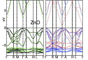
Figure 4: (Color online) Energy bands in wurzite ZnO. Solid(Black) in left panel:QSGW(‘mode-A’) ;  Broken(Green) in left:1shotNZ(off-d) ;  Solid(Blue) in right panel:‘e-only’ ;  Dotted(Red) in right panel:LDA.

Data for the direct gap at $\Gamma$ for wurzite ZnO, and for Cu₂O (cuprite structure) are given in Table 5. In these materials, ‘1shotNZ’ (and more so ‘1shot’) results are rather poor, as were ZnS and ZnSe (Table 4). Corresponding energy bands are shown in Figs. 4 and 6. We used 144 and 64 ${\bf k}$ points in the 1st BZ to make $H^{0}$ for ZnO and Cu₂O, respectively. ‘1shotNZ(off-d)’ denotes a 1shot calculation, including the off-diagonal elements of ${\it\Delta}V^{\rm xc}$ computed in ‘mode-A’; i.e. bands were generated by $H^{\rm LDA}+{\it\Delta}V^{\rm xc}$ without self-consistency. They differ little from standard ‘1shotNZ’ results in semiconductors, as we showed for variety of materials in Ref. van Schilfgaarde et al. . Calculated dielectric constants $\epsilon_{\infty}$ are shown in Table 6. Note its systematic underestimation. Data “With LFC” is the better calculation, as it includes the so-called local field correction (See e.g. Arnaud and Alouani (2001)).

III.4.1 ZnO

In contrast to cases in Sec. III.3 ‘e-only’ and ‘1shotNZ’ now show sizable differences. This is because the LDA gap is much too small, and $W$ is significantly overestimated. The discrepancy is large enough that ‘1shotNZ,’ which approximately corresponds to ‘e-only’ but neglecting changes in $W^{\rm LDA}$, is no longer a reasonable approximation. On the other band, Table 5 shows that the ‘e-only’ and ‘mode-A’ are not so different (3.64 eV compared to 3.87 eV). This difference measures the contribution of the off-diagonal part to band gap; it is similar to ZnS. This modest difference suggests that the LDA eigenfunctions are still reasonable. However, there still remains a difficulty in disentangling $d$ valence bands from the others in the ‘e-only’ case: topological connections in band dispersions can not be changed from the LDA topology, as we discussed in Ref. van Schilfgaarde et al. .

The imaginary part of the dielectric function, ${\rm{Im}}\,\epsilon({\bf{q}}$=${0},\omega)$, is calculated from the ‘mode-A’ potential and compared to the experimental function in Fig. 5. There is some discrepancy with experiment. Arnaud and Alouani Arnaud and Alouani (2001) calculated the excitonic contribution to ${\rm Im}\,\epsilon(\omega)$ with the Bethe-Salpeter equation for several semiconductors. Generally speaking, such a contribution can shift peaks in ${\rm{Im}}\,\epsilon({\bf{q}}$=${0},\omega)$ to lower energy and create new peaks just around the band edge. It is in fact just what is needed to correct the discrepancy with experiments as seen in Fig. 5.

Figure 5: (Color online) Imaginary part of dielectric function for ZnO. Local field corrections (LFC) only slightly affect the result.

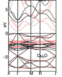
Figure 6: (Color online) Energy bands of Cu₂O. Dotted(Red):LDA ;  Solid(Black):QSGW(‘mode-A’).

Figure 7: Partial DOS (QP-DOS) computed from the QSGW $H^{0}$ for Cu₂O. Valence band maximum at zero. Right-hand scale is for unoccupied states and is 10$\times$ the left-hand scale, which applies to occupied states.

Figure 8: (Color online) Absorption coefficient for Cu₂O. Experiment is taken from Ref. Brahms et al. (1966).

III.4.2 Cu₂O

We have to distinguish between the QP density of states (QP-DOS), which is calculated from $H^{0}$ (the poles of $G^{0}$), and the “spectrum” density-of-states, which is calculated from the poles of $G$. The QP-DOS is the important quantity needed to describe the fundamental excitations in materials. QP-DOS in ‘mode-A’ are shown in Fig. 7. The absorption coefficient in RPA from $H^{0}$ is shown in Fig. 8, as well as the energy bands in Fig. 6. This calculation includes Cu3$p$ and Cu4$d$ as VAL states using local orbitals.

As shown in Table 5, the discrepancy between “e-only” and “mode-A” fundamental gap is $\sim$0.4 eV, rather significant and larger than cases considered previously. This reflects an increased discrepancy between the LDA and QSGW eigenfunctions. The ‘mode-A’ energy bands can be compared with results by Bruneval et al. Bruneval et al. (2006b), who also performed QSGW calculations within a pseudopotential framework. The lowest and second gaps we obtain, $E_{g}$=2.36 eV and $E_{0}$=2.81 eV, are somewhat larger than their values (1.97 eV and 2.27 eV). Further, the difference between the peaks just below $E_{\rm F}$ and the main $3d$ peak is 1.90 eV, which is slightly larger than what Bruneval et al. obtain (1.64 eV). This is the D1-F1 difference in Ref. Shen et al. (1990), measured to be 1.94 eV. The absorption coefficient shows essentially the same kinds of discrepancy with experiment as we saw for Im$\,\epsilon(\omega)$ in ZnO. Bruneval et al. calculated the excitonic contributions for Cu₂O in a Bethe-Salpeter framework Bruneval et al. (2006b), and showed that they account for most of the error in the RPA dielectric function as computed by QSGW.

III.5 NiO and MnO

We described these compounds already in Ref. Faleev et al. (2004); here we present some additional analysis. We assume antiferro-II ordering Terakura et al. (1984) and time-reversal symmetry (thus no orbital moments), with 64 ${\bf k}$-points in the 1st BZ. In Fig. 9, we show QSGW ‘mode-A’ energy bands, comparing them to ‘e-only’ and LDA in the right panel. The problem with ‘e-only’ bands is now very apparent: the bandgap is much too small and the conduction band dispersions are qualitatively wrong (minimum gap falls at the wrong point for NiO). Further, the valence bands (especially, the relative position of O 2$p$ and TM $3d$ bands) changes little relative to the LDA. ‘e-only’ can not change the LDA’s spin moment since eigenfunctions do not change; they are significantly underestimated. The QP-DOS are shown in Fig. 10. As we detail below, the self-consistency is essential for these materials as was found by Aryasetiawan and Gunnarsson Aryasetiawan and Gunnarsson (1995).

Figure 9: (Color online) Energy bands for NiO and MnO. Solid(Black) in left panel: QSGW(‘mode-A’) ; Solid(Blue) in right panel:‘e-only’ ; Dotted(Red) in right panel: LDA.

Figure 10: (Color online) QP-DOS(‘mode-A’) for NiO and MnO for each atomic site. Contributions are decomposed majority and minority in Mn(Ni) site in top two panels. Further, it is decomposed into $e_{g}$ and $t_{2g}$. Dotted(Red): $e_{g}$;  Solid(Black):$t_{2g}$. O(total) is the QP-DOS project onto an O site (sum of majority and minority). Dots(Red) in the bottom panels are taken from XPS+BIS experiments van Elp et al. (1991, 1992), and are compared with total QP-DOS broadened with a 0.6 eV Gaussian.

Figure 11: (Color online) Imaginary part of the dielectric function in MnO and NiO. Effects of local fields (LFs) are significant only in the deep energy region related to the $3p$ core (inset). LF effects contribute mainly to such local atomic-like excitations; they should be interpreted in terms of the Lorenz field in the Clausius-Mossotti relation. Local fields reduce the peaks of localized excitations, and moves them to higher energy (this is already seen in rutile TiO₂ Vast et al. (2002)). Experimental data is taken from Ref. Messick et al. (1972) for MnO, and Ref. Powell and Spicer (1970) for NiO.

III.5.1 MnO

The Mn $e_{g}$ and O $2p$ QP-DOS show common peaks below $E_{\rm F}$. This is because of the strong $dd_{\sigma}$ coupling between $e_{g}$, mediated through the O $2p$ valence bands Terakura et al. (1984). The $e_{g}$ components are separated mainly into two peaks which have comparable weight, in contradiction to the LDA case where the deeper peak has a very small weight. This is because $e_{g}$ levels are pushed down relative to the LDA. The bottom panel compares XPS (occupied states) and BIS (unoccupied states) experiments with the total QP-DOS, broadened with 0.6 eV Gaussian. There is good agreement with the XPS part for the $e_{g}$ peak just below $E_{\rm F}$, for the $t_{2g}$ peak, and for the valence band width. (Based on a model analysis by Takahashi and Igarashi Takahashi and Igarashi (1996), we expect that many-body effects do not strongly perturb the QP-DOS.) However, there is discrepancy in the BIS part. A possible assignment is to identify a shoulder of total QP-DOS seen at $\sim$ $E_{\rm F}$+7eV as the peak of the BIS at $\sim$ 6.8 eV (as claimed in Ref. Faleev et al. (2004)). Alternatively it is possible that the QP-DOS predicts conduction bands $\sim 1.5$eV higher than the BIS data.

Fig. 11 compares ${\rm{Im}}\epsilon(\omega)$ generated by QSGW ‘mode-A’ with experiment. The discrepancy looks too large to explain the difference between the ‘mode-A’ calculation and the experimental data. However, if we neglect the difference in absolute value, we can say that ‘mode-A’ predicts the peak ${\rm Im}\epsilon(\omega)$ at an energy too high by $\sim$2 eV. This view is consistent with the conjecture below for NiO.

III.5.2 NiO

The majority-spin QP-DOS of NiO is roughly similar to that of MnO. However, the $e_{g}$ state just below $E_{\rm F}$ is broadened and carries less weight (Fig. 10). That peak is seen in MnO but is lost in this case, though the deeper $e_{g}$ peak remains. The $t_{2g}$ DOS is widened relative to LDA. These features are also observed in other beyond-LDA calculations Massidda et al. (1997); Bengone et al. (2000). The top of valence consists of O $2p$ states, which hybridize with majority $e_{g}$ states, and minority $t_{2g}$ which weakly hybridize. In the bottom panel, the $d$ DOS between $E_{\rm F}$ and $E_{\rm F}$$-$4eV falls in good agreement with XPS; but the valence DOS width differs from XPS, in contradistinction to MnO. The reason can be attributed to the satellite structure contained in the XPS data: e.g. Takahashi et al. Takahashi and Igarashi (1996) predict that a satellite should appear around $E_{\rm F}$$-$9eV.

Turning to the unoccupied states, we can see ‘mode-A’ puts a peak $\sim$1.3 eV too high compared BIS peak at $\sim$$E_{\rm F}$$+$5eV. On the other hand, ${\rm{Im}}\epsilon(\omega)$ is in rather reasonable agreement with experiment except for a shift in the first peak by $\sim$2.0 eV (‘mode-A’). Thus we can distinguish two kinds errors in bandgap: (1.3 eV in BIS, and 2.0 eV in Im$\epsilon$). We think both kinds of errors can be explained by the excitonic effects for $W$ missing in our QSGW calculation. This is consistent with the QSGW $\epsilon_{\infty}$ being underestimated. Thus our conjecture is: if we properly include the excitonic contributions to $W$, weights in Im$\epsilon$ will shift to lower energy, increasing $\epsilon_{\infty}$. Self-consistency with such $W$ should reduce the band gap, simultaneously improving agreement with BIS and the dielectric function.

III.6 Fe and Ni

Fig. 12 shows energy bands for Fe and Ni calculated by LDA, QSGW ‘mode-A’ and ‘e-only’. The two QSGW calculations show similar $d$ band shapes: their widths narrow relative to LDA, moving into closer agreement with experiment. On the other hand, the ‘e-only’ calculation significantly shifts the relative positions of the $s$ and $d$ levels, depressing the bottom of $s$ band $\sim$1 eV in contradiction to experiment. ‘1shotNZ’ results (not shown) are very similar to the ‘e-only’ case. This indicates the importance of the charge redistribution due to the off-diagonal part of Eq. (10) in the 3$d$ transition metals. Yamasaki and Fujiwara Yamasaki and Fujiwara (2003) presented the ‘1shot’ $GW$​A results for Fe, Ni, and Cu, Aryasetiawan Aryasetiawan (1992) for Ni. Both calculations included the $Z$ factor ($Z\approx 0.8$ for $s$ band, $Z\approx 0.6$ for $d$ band) thus the changes they found relative to LDA are not so large. Including the $Z$ factor mostly eliminates the unwonted $s$ band shift. However it does so apparently fortuitously. As ‘1shot’ (and ‘1shotNZ’) should be taken as an approximation of ‘e-only’, it is wrong to take ‘1shot’ as a better theoretical prediction than ‘e-only’. The calculated spin magnetic moments are listed in Ref. van Schilfgaarde et al. (2006). Little difference with experiment is found for Fe (2.2 $\mu_{\rm B}$). For Ni, QSGW gives 0.7$\mu_{\rm B}$, a little larger than the experimental value 0.6 $\mu_{\rm B}$. This is reasonable because QSGW does not include the effect of spin fluctuations.

Figure 12: (Color online) Energy bands for Fe and Ni. Solid(Black): QSGW(‘mode-A’) ;  Broken(Blue): ‘e-only’ ;  Dotted(red): LDA. Calculations used $12\mbox{$\times$}12\mbox{$\times$}12=1728$ ${\bf k}$-points in the 1st BZ. Comparing to calculations at other $k$ meshes $8\mbox{$\times$}8\mbox{$\times$}8\dots 14\mbox{$\times$}14\mbox{$\times$}14$, we estimate the numerical convergence is a little better than 0.1 eV. In this case convergence is limited by uncertainties in the determination $E_{\rm F}$ met . Inspection of the bands at fine resolution show slight discontinuities at certain $k$ points. These occur at times because of difficulties in the $\Sigma$ interpolation; see Sec. II.7 and the smearing procedure in Sec. II.5.

IV summary

We showed that the QSGW formalism can be derived from a standpoint of self-consistent perturbation theory, where the unperturbed Hamiltonian is an optimized noninteracting one. Then we presented a means to calculate the total energy based on adiabatic connection, and how it relates to the density functional framework.

We then showed a number of key points in the implementation of our all-electron $GW$A and QSGW. The mixed basis for $W$ and the offset-$\Gamma$ method are especially important technical points. We presented some convergence checks for the mixed basis, and some results in various kinds of systems to demonstrate how well QSGW works. For insulators, QSGW provides rather satisfactory description of valence bands; conduction bands are also well described though bandgaps are systematically overestimated slightly. We compared the difference of the QSGW results to eigenvalue-only self-consistent results and to 1shot-$GW$ results in various cases.

How well eigenvalue-only self-consistency works depends on how correlated the system is. In covalent semiconductors LDA eigenfunctions are rather good, and there is little difference. The error is no longer small in Cu₂O, Fe, and Ni; finally eigenvalue-only self-consistency fails qualitatively in NiO.

We would like to thank F. Aryasetiawan for giving us his LMTO-ASA $GW$ code, which formed the basis for development of the present one. This work was supported by the DARPA SPINS project, and by ONR contract N00014-02-1-1025. We thank the Fulton HPC for computational resources used in this project.

Appendix A How to justify $G^{0}W^{0}$ approximation from $\Sigma[G]$? — Z factor cancellation

We explain the “$Z$ factor cancellation”, which is one justification for so-called $G^{0}W^{0}$ approximation. To the best of our knowledge, it is not clearly discussed in spite of its importance. Hereafter, $W$ and $\Pi$ denote the dynamical screened Coulomb interaction, and the proper polarization function without approximation; $W^{0}$ and $\Pi^{0}$ denote the same in RPA. It gets clearer that the well-balanced treatment between the vertex function $\Gamma$ and $G$ to respect “$Z$ factor cancellation” is important; thus the so-called full self-consistent $GW$ Holm and von Barth (1998); Zein and Antropov (2002); Ku and Eguiluz (2002); Biermann et al. (2003); Stan et al. (2006) must be a problematic approximation. We will use symbolical notations hereafter for simplicity.

As is well known, the exact self energy $\Sigma$ is calculated from $G$ as $\Sigma=GW\Gamma$ Hedin (1965). $G$ can be written as

$$G=ZG^{0}+\bar{G},$$ (60)

where $G^{0}$ is the QP part of the Green’s function, $Z$ is the renomalization factor, and $\bar{G}$ is the incoherent part. The incoherent part contains physically unclear kinds of intermediate states, which are not always characterizable by a single-particle propagator.

In (a) below, we consider the $Z$-factor cancellation in the calculation of $\Sigma=GW\Gamma$ for given $G$, $W$, and $\Gamma$ and in (b), the $Z$ factor cancellation in $\Pi$.

• In the integration of $GW\Gamma$, the most dominant part is related to the long range static part of $W$, the ${\bf q}\to 0$ and $\omega\to 0$ limit of $W({\bf q},\omega)$. In this limit, the vertex function becomes

  $$\Gamma\to 1-\frac{\partial\Sigma}{\partial\omega}=1/Z.$$ (61)

  This is a Ward identity. Here we need to assume the insulator case. Then there is a cancellation between $Z$ from $ZG^{0}$ and $1/Z$ from $\Gamma$. Under the assumption that $\bar{G}$ is rather structureless, $\bar{G}W$ may give almost state-independent contributions (may results in a little changes of chemical potential), thus $GW\Gamma\approx G^{0}W$ is essentially satisfied. In the case of metal, there is an additional term in right-hand side of Eq. (61) due to the exsitence of the Fermi surface; then we expect $\Gamma>1/Z$, see e.g. Nozieres (1964); the point (b) below should be interpreted in the same manner. In any cases, we can claim the poorness of fully self-consistent $GW$ which neglect $\Gamma$, as discussed in the follwing.

• $W$ is given in terms of the proper polarization function $\Pi$ as $W=v(1-v\Pi)^{-1}$. $\Pi(1,4)=\bar{\Pi}(1,1;4,4)$, which is written as

  $$\bar{\Pi}(1,1^{\prime};4,4^{\prime})=G_{2}(1,1^{\prime};4,4^{\prime})+G_{2}(1,1^{\prime};2,2^{\prime})I(2,2^{\prime};3,3^{\prime})\bar{\Pi}(3,3^{\prime};4,4^{\prime})$$

  $$=G_{2}+G_{2}IG_{2}+G_{2}IG_{2}IG_{2}+\dots.$$ (62)

  Here $G_{2}(1,1^{\prime};2,2^{\prime})=-iG(1,2)G(2^{\prime},1^{\prime})$, and the duplicated indices are integrated (the Einstein sum rule). This looks like an electron-hole ladder diagram, but with the two-particle irreducible kernel $I(1,1^{\prime};2,2^{\prime})$ playing the role of the steps of the ladder. $G_{2}$ contains an electron-hole pair excitation $\Psi_{i}({\bf r}_{1})\Psi_{i}^{*}({\bf r}_{1}^{\prime})\Psi_{j}^{*}({\bf r}_{2})\Psi_{j}({\bf r}_{2}^{\prime})\times(n_{j}-n_{i})\delta(\omega-(\varepsilon_{i}-\varepsilon_{j}))$ multipled by $Z^{2}$ in its intermediate state (imaginary part), because $G_{2}$ contains $ZG^{0}\times ZG^{0}$. Here $\varepsilon_{i}$ and $\Psi_{i}$ denote a QPE and QP eigenfunction included in $G^{0}$, and $n_{j}-n_{i}$ is the occupation number difference.

  Let us consider how much the pair excitation is included in $\bar{\Pi}$ (i.e. how $\bar{\Pi}(1,2;3,4)$ changes when a pair excitation is added or removed) in its intermediate states. This means take the derivative of $\bar{\Pi}$ through $G_{2}$ with respect to $n_{j}-n_{i}$ (derivative is not through $I$. Such contribution is not two-particle reducible, that is, not for the intermediate states for $\bar{\Pi}$).

  We can show that

  $${\it\Delta}\Pi(1,4)=\Gamma(1,2,2^{\prime}){\it\Delta}G_{2}(2,2^{\prime};3,3^{\prime})\Gamma(4,3^{\prime},3)$$

  ;this is derived from Eq. (62) with paying attention to the matrix notation; $\Gamma(1,2,2^{\prime})=\frac{1}{1-G_{2}I}$ and $\Gamma(4,3^{\prime},3)=\frac{1}{1-IG_{2}}$ symbolically. Thus we see that the additional pair excitation (intermediate state) is included in $\Pi$ with the weight $\frac{1}{Z}\times Z^{2}\times\frac{1}{Z}=1$ for ${\bf q}\to{}0,\omega\to{}0$, because of Eq. (61) (factors ${1}/{Z}$ come from $\Gamma$). This is the $Z$ factor cancellation mechanism for $\bar{\Pi}$. Bechstedt et al. demonstrated this in practice Bechstedt et al. (1997) at the lowest level of approximation.

  This suggests that $\Pi(1,2)\approx\Pi^{0}(1,2)=-iG^{0}\times G^{0}$ is a reasonable approximation because the derivative of $\Pi^{0}(1,2)$ apparently does not include any $Z$ factor — thus the $Z$ factor cancellation is trivially satisfied.

In the above discussion, we use the fact that $GW$A is dominated by the long range part of $W$; we may expect such $Z$ cancellation somehow occurs even for short-range $W$; but it may be less meaningful. The above discussion shows why the fully self-consistent $GW$ method is a poor approximation. Because the vertex function is omitted, $Z$ in $G=ZG^{0}+\bar{G}$ is not canceled. $\Sigma=\frac{\delta E_{\rm xc}[G]}{\delta G}$ must be a rigorous formula; however, the series expansion in $G$ should be very inefficient — it contains rather large cancellations between terms in the series so as to cancel out the effect of $Z$ as seen in (a) and (b).

On the other hand, the $G^{0}W^{0}$ approximation looks reasonable from the viewpoint of (a) and (b), because it includes contributions from QPs with correct weights. From the beginning, this is what we expect from the Landau-Silin QP picture.

$Z$ factor cancellation is generally important. For example, the Bethe-Salpeter equation (BSE) can be described as the sum of the ladder diagrams; if $G$ is used instead of $G^{0}$ in the sum, it should give a similarly poor result.

To summarize, it looks more reasonable to calculate $\Sigma[G]$ through the QP part $G^{0}$ contained in $G$. That is, $G\to G^{0}\to\Sigma$, where we can use $G^{0}W^{0}$ approximation for $G^{0}\to\Sigma$. From this $\Sigma$, we can calculate a new $G$; this suggest the self-consistency cycle $G\to G^{0}\to G\to G^{0}...$. The problem is how to extract $G^{0}$ from $G$; the QSGW method gives a (nearly) optimal prescription.

Mahan and Sernelius Mahan and Sernelius (1989) also emphasized the balanced treatment of the vertex function and $W$. Their work however, is not directly related to the discussion here. Their calculation is not based on $GW\Gamma$; instead they use $G^{0}$, and their vertex at ${\bf q}\to 0$ is not $1/Z$, but unity. Their formula is based on the derivative of the $G^{0}$-based total energy with respect to the occupation number Quinn and Ferrell (1958). Their vertex function is identified as the correction to modify $W$ into the effective interaction between a test charge and a QP. Their formula (or originally from Quinn et al. Quinn and Ferrell (1958)) is related to the discussion in Appendix B.

Appendix B Can we determine $G$ by total energy minimization?

The RPA total energy Eq. (22) can be taken as a functional of $V^{\rm eff}({\bf r},{\bf r}^{\prime})$: $E^{\rm RPA}$ depends on $V^{\rm eff}({\bf r},{\bf r}^{\prime})$ through $G^{0}$. Note that the HF part of the total energy does not explicitly include QPEs (eigenvalues of $H^{0}$), but $E^{\rm c,RPA}$ does include them.

In contradiction to the local potential case as, e.g. in the Kohn-Sham construction of DFT, it is meaningless to minimize $E^{\rm RPA}$ with respect to $V^{\rm eff}({\bf r},{\bf r}^{\prime})$. $V^{\rm eff}({\bf r},{\bf r}^{\prime})$ contains degree of freedom that can shift QPEs while keeping the eigenfunctions fixed (This is realized by adding a potential propotional to $\psi_{i}({\bf r})\psi^{*}_{i}({\bf r}^{\prime})$). Thus it is possible to change only $E^{\rm c,RPA}$ by varying $V^{\rm eff}({\bf r},{\bf r}^{\prime})$ in such a way that QPEs change but not eigenfunctions. This implies that $E^{\rm c,RPA}$ can be infinite (no lower bound) when all QPEs are moved to the Fermi energy.

On the other hand, it is possible to determine a QPE from the functional derivative of $E^{\rm RPA}$ with respect to the occupancy of a state $\Psi_{i}$. It gives the QPE as $\varepsilon_{i}=\frac{\partial E^{\rm RPA}}{\partial n_{i}}$ Quinn and Ferrell (1958). This is in agreement with QPE calculated by $GW$A starting from $H^{0}$. Thus, under the fixed QP eigenfunctions, we can determine QPEs self-consistently; we use these $\varepsilon_{i}$ in $E^{\rm RPA}$ and take its derivative with respect to $\Psi_{i}$ to determine the next $\varepsilon_{i}$ — this is repeated until converged. This is nothing but the eigenvalue-only self-consistent scheme. QPE are not determined by the total energy minimization: that is QPEs are not variational parameters. Nevertheless it is a self-consistency condition (consistency for the excitations around the ground state) and it is meaningful.

Therefore, we can calculate $E^{\rm RPA}$ for a given complete set of QP eigenfunctions, where QPEs are made self-consistent in the manner above. It will be possible to minimize this $E^{\rm RPA}$ with respect to the set of QP eigenfunctions. However, such a formalism looks too complicated. Further, only the occupied QP eigenfunctions are included in the Hartree-Fock part of $E^{\rm RPA}$; thus, continuity (smoothness) from the occupied eigenfunctions to unoccupied eigenfunctions will be lost. Thus we think that it is better to choose another possibility, namely to determine not only QPEs but also the QP eigenfunctions in the self-consistency cycle, as we do in QSGW.

References

- Hedin (1965) L. Hedin, Phys. Rev. 139, A796 (1965).
- Strinati et al. (1980) G. Strinati, H. J. Mattausch, and W. Hanke, Phys. Rev. Lett. 45, 290 (1980).
- Pickett and Wang (1984) W. E. Pickett and C. S. Wang, Phys. Rev. B 30, 4719 (1984).
- Hybertsen and Louie (1986) M. S. Hybertsen and S. G. Louie, Phys. Rev. B 34, 5390 (1986).
- Hohenberg and Kohn (1964) P. Hohenberg and W. Kohn, Phys. Rev. 136, B864 (1964).
- Kohn and Sham (1965) W. Kohn and L. J. Sham, Phys. Rev. 140, A1133 (1965).
- Aryasetiawan and Gunnarsson (1998) F. Aryasetiawan and O. Gunnarsson, Rep. Prog. Phys 61, 237 (1998).
- Kotani and van Schilfgaarde (2002) T. Kotani and M. van Schilfgaarde, Solid State Commun. 121, 461 (2002).
- Usuda et al. (2004) M. Usuda, H. Hamada, K. Siraishi, and A. Oshiyama, Jpn. J. Appl. Phys. Lett. (part 2) 43, L407 (2004).
- Fleszar and Hanke (2005) A. Fleszar and W. Hanke, Phys. Rev. B 71, 045207 (2005).
- (11) M. van Schilfgaarde, T. Kotani, and S. V. Faleev, phys. Rev. B. (2006), in press. Preprint cond-mat/0508295.
- Surh et al. (1991) M. P. Surh, S. G. Louie, and M. L. Cohen, Phys. Rev. B 43, 9126 (1991).
- Luo et al. (2002) W. Luo, S. Ismail-Beigi, M. L. Cohen, and S. G. Louie, Phys. Rev. B 66, 195215 (2002).
- Aryasetiawan and Gunnarsson (1995) F. Aryasetiawan and O. Gunnarsson, Physical Review Letters 74, 3221 (1995), URL http://link.aps.org/abstract/PRL/v74/p3221.
- Faleev et al. (2004) S. V. Faleev, M. van Schilfgaarde, and T. Kotani, Phys. Rev. Lett. 93, 126406 (2004).
- van Schilfgaarde et al. (2006) M. van Schilfgaarde, T. Kotani, and S. Faleev, Phys. Rev. Lett. 96, 226402 (pages 4) (2006), URL http://link.aps.org/abstract/PRL/v96/e226402.
- Chantis et al. (2006a) A. N. Chantis, M. van Schilfgaarde, and T. Kotani, Phys. Rev. Lett. 96, 086405 (2006a), URL http://link.aps.org/abstract/PRL/v96/e086405.
- Chantis et al. (2006b) A. N. Chantis, M. van Schilfgaarde, and T. Kotani (2006b), submitted.
- Bruneval et al. (2006a) F. Bruneval, N. Vast, and L. Reining, Physical Review B (Condensed Matter and Materials Physics) 74, 045102 (pages 15) (2006a), URL http://link.aps.org/abstract/PRB/v74/e045102.
- Alouani and Wills (1996) M. Alouani and J. M. Wills, Phys. Rev. B 54, 2480 (1996).
- Arnaud and Alouani (2001) B. Arnaud and M. Alouani, Phys. Rev. B 63, 085208 (2001).
- Mahan (1990) G. D. Mahan, Many-Particle Physics (Plenum Press, New York, 1990).
- Kotani (1998) T. Kotani, J.Phys.: Condens. Matter 10, 9241 (1998).
- Pines and Nozieres (1966) D. Pines and P. Nozieres, The Theory of Quantum Liquid. Vol I (W.A.Benjamin Inc., New York, 1966).
- Ashcroft and Mermin (1976) N. W. Ashcroft and D. N. Mermin, Solid State Physics (Brooks Cole, 1976).
- Fischetti and Laux (1988) M. V. Fischetti and S. E. Laux, Phys. Rev. B 38, 9721 (1988).
- Schöne and Eguiluz (1998) W.-D. Schöne and A. Eguiluz, Phys. Rev. Lett 81, 1662 (1998).
- Ku and Eguiluz (2002) W. Ku and A. G. Eguiluz, Phys. Rev. Lett. 89, 126401 (2002).
- Baym and Kadanoff (1961) G. Baym and L. P. Kadanoff, Phys. Rev. 124 (1961).
- Fukuda et al. (1994) R. Fukuda, T. Kotani, Y. Suzuki, and S. Yokojima, Prog. Theor. Phys. 92, 833 (1994).
- Bechstedt et al. (1997) F. Bechstedt, K. Tenelsen, B. Adolph, and R. D. Sole, Phys. Rev. Lett. 78, 1528 (1997).
- Springer et al. (1998) M. Springer, F. Aryasetiawan, and K. Karlsson, Phys. Rev. Lett. 80, 2389 (1998).
- Biermann et al. (2003) S. Biermann, F. Aryasetiawan, and A. Georges, Phys. Rev. Lett. 90, 086402 (2003).
- Mahan and Sernelius (1989) G. D. Mahan and B. E. Sernelius, Phys. Rev. Lett. 62, 2718 (1989).
- Fuchs and Gonze (2002) M. Fuchs and X. Gonze, Phys. Rev. B 65, 235109 (2002).
- Miyake et al. (2002) T. Miyake, F. Aryasetiawan, T. Kotani, M. van Schilfgaarde, M. Usuda, and K. Terakura, Phys. Rev. B 66, 245103 (2002).
- Aryasetiawan et al. (2002) F. Aryasetiawan, T. Miyake, and K. Terakura, Phys. Rev. Lett. 88 (2002).
- Marini et al. (2006) A. Marini, P. García-González, and A. Rubio, Phys. Rev. Lett. 96, 136404 (2006).
- Sakuma et al. (2006) R. Sakuma, S. Tsuneyuki, T. Kotani, M. van Schilfgaarde, and T. Miyake, unpublished (2006).
- Methfessel et al. (2000) M. Methfessel, M. van Schilfgaarde, and R. A. Casali, in Lecture Notes in Physics, edited by H. Dreysse (Springer-Verlag, Berlin, 2000), vol. 535.
- Bott et al. (1998) E. Bott, M. Methfessel, W. Krabs, and P. C. Schmidt, J. Math. Phys. 39, 3393 (1998).
- Usuda et al. (2002) M. Usuda, N. Hamada, T. Kotani, and M. van Schilfgaarde, Phys. Rev. B 66, 125101 (2002).
- Friedrich et al. (2006) C. Friedrich, A. Schindlmayr, S. Blügel, and T. Kotani, Phys. Rev. B 74, 045104 (2006).
- (44) In the scheme as we have currently implemented it, CORE wave function can be obtained subject to the boundary condition that the value and slope vanish at the MT boundary. This procedure do not assure the orthogonality between CORE and VAL (the importance of orthogonality is seen at limit in dielectric function); this can be a source of error in the present treatment of CORE.
- Aryasetiawan and Gunnarsson (1994) F. Aryasetiawan and O. Gunnarsson, Phys. Rev. B 49, 16214 (1994).
- Rath and Freeman (1975) J. Rath and A. Freeman, Phys. Rev. B 11, 2109 (1975).
- Miyake and Aryasetiawan (2000) T. Miyake and F. Aryasetiawan, Phys. Rev. B 61, 7172 (2000).
- Lebègue et al. (2003) S. Lebègue, B. Arnaud, M. Alouani, and P. E. Bloechl, Phys. Rev. B 67, 155208 (2003).
- Yamasaki and Fujiwara (2003) A. Yamasaki and T. Fujiwara, J. Phys. Soc. Japan 72, 607 (2003).
- Gygi and Baldereschi (1986) F. Gygi and A. Baldereschi, Phys. Rev. B 34, 4405 (1986).
- Godby et al. (1988) R. W. Godby, M. Schlüter, and L. J. Sham, Phys. Rev. B 37, 10159 (1988).
- Aryasetiawan (2000) F. Aryasetiawan, The GW approximation and vertex correction (G & B Science Pub, 2000).
- Kotani (2000) T. Kotani, J.Phys. Cond. Mat. 12 (2000).
- (54) There is some ambiguity in the metal case, about whether it is better to use the same mesh in both the “small loop” and the generation of , or to use a finer mesh for a given . The consistent mesh is preferable in that states above and below are counted in a consistent way; i.e. there is a consistency between and . Using a finer mesh for the small loop is preferable because the kinetic energy is a much more sensitive function of Fermi-surface effects than , which is determined by the small loop. Using a consistent mesh that is well converged in the kinetic energy can require unrealistically large numbers of points (something like 163 points in Fe for 0.01 eV accuracy). Usually the amgibuity is rather small on the scale of other uncertainties in the calculation.
- Andersen et al. (2000) O. K. Andersen, T. Saha-Dasgupta, R. W. Tank, and G. K. C. A. O. Jepsen, in Lecture Notes in Physics, edited by H. Dreysse (Springer-Verlag, Berlin, 2000), vol. 535.
- Hamada et al. (1990) N. Hamada, M. Hwang, and A. J. Freeman, Phys. Rev. B 41, 3620 (1990), URL http://link.aps.org/abstract/PRB/v41/p3620.
- Cardona and Thewalt (2005) M. Cardona and M. L. W. Thewalt, Rev. Mod. Phys. 77, 1173 (2005).
- Adachi (2004) S. Adachi, Handbook On Physical Properties Of Semiconductors, vol. 3 (Kluwer Academic, Boston, 2004).
- Madelung (1996) O. Madelung, Semiconductors Basic Data (Springer-Verlag, Berlin, 1996).
- Jiménez et al. (1997) I. Jiménez, L. J. Terminello, D. G. J. Sutherland, J. A. Carlisle, E. L. Shirley, and F. J. Himpsel, Phys. Rev. B 56, 7215 (1997).
- Logothetidis et al. (1992) S. Logothetidis, J. Petalas, H. M. Polatoglou, and D. Fuchs, Phys. Rev. B 46, 4483 (1992).
- Himpsel et al. (1979) F. J. Himpsel, J. A. Knapp, J. A. VanVechten, and D. E. Eastman, Phys. Rev. B 20, 624 (1979).
- Lautenschlager et al. (1987a) P. Lautenschlager, M. Garriga, L. Vina, and M. Cardona, Phys. Rev. B 36, 4821 (1987a).
- (64) Crystal and Solid State Physics, Vol. 22A, Landolt-Börnstein; Numerical Data and Functional Relationships in Science and Technology edited by O. Madelung (Springer, Berlin, 1984).
- Kraut et al. (1980) E. A. Kraut, R. W. Grant, J. R. Waldrop, and S. P. Kowalczyk, Phys. Rev. Lett. 44, 1620 (1980).
- Ley et al. (1974) L. Ley, R. A. Pollak, F. R. McFeely, S. P. Kowalczyk, and D. A. Shirley, Phys. Rev. B 9, 600 (1974).
- Lautenschlager et al. (1987b) P. Lautenschlager, M. Garriga, S. Logothetidis, and M. Cardona, Phys. Rev. B 35, 9174 (1987b).
- Zhou et al. (1997) L. Zhou, T. A. Callcott, J. J. Jia, D. L. Ederer, and R. Perera, Phys. Rev. B 55, 5051 (1997).
- Mang et al. (1996) A. Mang, K. Reimann, S. Rübenacke, and M. Steube, Phys. Rev. B 53, 16283 (1996).
- Vesely et al. (1972) C. J. Vesely, R. L. Hengehold, and D. W. Langer, Phys. Rev. B 5, 2296 (1972).
- Markowski et al. (1994) R. Markowski, M. Piacenti, D. Debowska, M. Zimnal-Starnawska, F. Lama, N. Zema, and A. Kisiel, J. Phys.: Cond. Mat. 6, 3207 (1994).
- Dougherty et al. (1997) D. J. Dougherty, S. B. Fleischer, E. L. Warlick, J. L. House, G. S. Petrich, L. A. Kolodziejski, and E. P. Ippen, Appl. Phys. Lett. 71, 3144 (1997).
- Adachi and Taguchi (1991) S. Adachi and T. Taguchi, Phys. Rev. B 43, 9569 (1991).
- Moriya et al. (2000) H. Moriya, A. Kaneta, and S. Adachi, Mater. Sci. Eng. B 76, 232 (2000).
- (75) Both numerator and denominator in the calculation of vanish as and . Thus we need to carefully extrapolate to from . But we found that just using a.u. is usually good sufficient to determine to one-tenth of digit for these cases without any numerical difficulties.
- Hodby et al. (1976) J. W. Hodby, T. E. Jenkins, C. Schwab, H. Tamura, and D. Trivich, J. Phys. C: Solid State Phys. 9, 1429 (1976).
- Mochizuki (1989) S. Mochizuki, J. Phys.: Condens. Matter 1 (1989).
- Plendl et al. (1969) J. N. Plendl, L. C. Mansur, S. S. Mitra, and I. F. Chang, Solid State Communications 7, 109 (1969).
- Powell and Spicer (1970) R. J. Powell and W. E. Spicer, Phys. Rev. B 2, 2182 (1970).
- Brahms et al. (1966) S. Brahms, S. Nikitine, and J. Dahl, Physics Letters 22, 31 (1966).
- Bruneval et al. (2006b) F. Bruneval, N. Vast, L. Reining, M. Izquierdo, F. Sirotti, and N. Barrett, Physical Review Letters 97, 267601 (pages 4) (2006b), URL http://link.aps.org/abstract/PRL/v97/e267601.
- Shen et al. (1990) Z.-X. Shen, R. S. List, D. S. Dessau, F. Parmigiani, A. J. Arko, R. Bartlett, B. O. Wells, I. Lindau, and W. E. Spicer, Phys. Rev. B 42, 8081 (1990).
- Terakura et al. (1984) K. Terakura, T. Oguchi, A. R. Williams, and J. Kübler, Phys. Rev. B 30, 4734 (1984).
- van Elp et al. (1991) J. van Elp, R. H. Potze, H. Eskes, R. Berger, and G. A. Sawatzky, Phys. Rev. B 44, 1530 (1991).
- van Elp et al. (1992) J. van Elp, H. Eskes, P. Kuiper, and G. A. Sawatzky, Phys. Rev. B 45, 1612 (1992).
- Vast et al. (2002) N. Vast, L. Reining, V. Olevano, P. Schattschneider, and B. Jouffrey, Phys. Rev. Lett. 88, 037601 (2002).
- Messick et al. (1972) L. Messick, W. C. Walker, and R. Glosser, Phys. Rev. B 6, 3941 (1972).
- Takahashi and Igarashi (1996) M. Takahashi and J. Igarashi, Phys. Rev. B 54, 13566 (1996).
- Massidda et al. (1997) S. Massidda, A. Continenza, M. Posternak, and A. Baldereschi, Phys. Rev. B 55, 13494 (1997).
- Bengone et al. (2000) O. Bengone, M. Alouani, P. Blochl, and J. Hugel, Phys. Rev. B 62, 16392 (2000).
- Aryasetiawan (1992) F. Aryasetiawan, Phys. Rev. B 46, 13051 (1992).
- Holm and von Barth (1998) B. Holm and U. von Barth, Phys. Rev. B 57, 2108 (1998).
- Zein and Antropov (2002) N. E. Zein and V. P. Antropov, Phys. Rev. Lett. 89, 126402 (2002).
- Stan et al. (2006) A. Stan, N. E. Dahlen, and R. van Leeuwen, Europhysics Lett. 76, 298 (2006).
- Nozieres (1964) P. Nozieres, Interacting Fermi Systems (W.A.Benjamin Inc., New York, 1964).
- Quinn and Ferrell (1958) J. J. Quinn and R. A. Ferrell, Phys. Rev. 112, 812 (1958).