Geometric treatment of electromagnetic phenomena in conducting materials: variational principles

Abstract

The dynamical equations of an electromagnetic field coupled with a conducting material are studied. The properties of the interaction are described by a classical field theory with tensorial material laws in space-time geometry. We show that the main features of superconducting response emerge in a natural way within the covariance, gauge invariance and variational formulation requirements. In particular, the Ginzburg-Landau theory follows straightforward from the London equations when fundamental symmetry properties are considered. Unconventional properties, such as the interaction of superconductors with electrostatic fields are naturally introduced in the geometric theory, at a phenomenological level. The BCS background is also suggested by macroscopic fingerprints of the internal symmetries.

It is also shown that dissipative conducting behavior may be approximately treated in a variational framework after breaking covariance for adiabatic processes. Thus, nonconservative laws of interaction are formulated by a purely spatial variational principle, in a quasi-stationary time discretized evolution. This theory justifies a class of nonfunctional phenomenological principles, introduced for dealing with exotic conduction properties of matter [Phys. Rev. Lett. 87, 127004 (2001)].

To be published: J. Phys. A: Math. Gen.

1 Introduction

Classical electrodynamics has been a commonplace in several areas of mathematical physics. Thus, many of the physical problems linked to the applications of function theory or differential geometry are taken from electromagnetism. In particular, we recall the very elegant formulation of the electromagnetic (EM) field in space time geometry. The full set of Maxwell equations may be simply expressed as $d{\cal F}=0$ and $\delta{{\cal F}}={{\cal J}}$, for ${{\cal F}}$ (the electromagnetic field tensor) a closed 2-form defined on the 4-dimensional Minkowski space, ${\cal J}$ the current density 1-form, and $\delta$ the so-called codifferential operator [1]. The closedness condition of ${\cal F}$ ($d{\cal F}=0$) allows a local representation in terms of a potential 1-form ${\cal A}$, introduced by ${\cal F}=d{\cal A}$. Maxwell laws may then arise as the Euler–Lagrange equations for an action functional in terms of ${\cal A}$. Within this geometric formulation of electromagnetism, the consideration of symmetry properties simplifies and illuminates the theory. In particular, covariance (which assures invariance of the equations under transformations of the Lorentz group) is very convenient and gauge invariance (invariance under transformations of the potential ${\cal A}\mapsto{\cal A}+d\chi$) must be satisfied.

All the above ideas are mainly established in the study of the electromagnetic (EM) field in vacuum, but can also be of great help in the research of interactions with electric charges within macroscopic media. Thus, it is known that the most relevant aspects of superconductivity: expulsion of magnetic fields, zero resistance, flux quantization and the phase-voltage relationship at the gap between superconductors, may be straightforwardly obtained from gauge invariance considerations [2].

Recently, and motivated by some experimental puzzles in superconducting physics, several additional tools, conventionally restricted to the research of EM fields and sources in vacuum, have been applied for the description of material laws. To be specific, space time covariance of the phenomenological equations of superconductivity has been considered as the appropriate framework for explaining the still unclear interaction of these materials with electrostatic fields. Essentially, and inspired in the principle of Lorentz covariance, when the electric and magnetic fields are treated at the same level, one predicts both electrostatic and magnetostatic field expulsion with a common penetration depth $\lambda$ [3, 4, 5]. This formulation has been used [6] as a basis for explaining the so-called Tao Effect, an intriguing experimental observation, in which superconducting microparticles aggregate into balls in the presence of electrostatic fields [7]. However, both theoretical objections [8] as well as experimental results [9] raise concerns on the universality of the common $\lambda$ treatment.

We want to emphasize that the topic of electrostatic field expulsion was already addressed by the London brothers [10] in the early days of superconductivity. Nonetheless, owing to the lack of experimental confirmation [11], they eventually decided to formulate their celebrated equations of superconductivity in a noncovariant form. Such a lack of relativistic covariance leads to theoretical difficulties, but they are conventionally avoided by postulating the absence of electrostatic charges and fields within the sample. This point of view has been adopted by the scientific community over decades, until the revived interest mentioned in the previous paragraph.

In the light of the above comments, it is apparent that finding a physically sound covariant expression for the material physical laws, in intrinsic geometric terms may be of help. In fact, it will be shown that this will not only release the theoretical dissatisfaction caused by using a somehow amended theory, but it will also allow to incorporate new physical phenomena in a natural way. In an effort to produce the most concise and general equations, we propose in this work, the use of differential forms on Minkowski space, within the area of electrical conductivity. However, it should be emphasized that relativistic exactitude is not meant to influence the kinetics of superconducting carriers. What one tries to do is to write the physics in the clearest form so as to get information on the underlying mechanism, through the macroscopic (phenomenological) electrodynamics. Being electrodynamics a fundamental interaction in the case of superconductors, one tries to scrutinize within the nature of the phenomenon, taking advantage of the EM field symmetries.

As a first approximation to the problem, we will restrict ourselves to linear effects in the material response, i.e. nonelectromagnetic degrees of freedom enter through the linear laws ${\cal J}=\Theta\cdot{\cal F}$ or ${\cal J}=\Xi\cdot{\cal A}+\omega$, with $\Theta\in{\cal T}_{1}^{\,2}$ and $\Xi\in{\cal T}_{1}^{\,1}$ field-independent tensors, and $\omega$ a gauge adjusting 1-form. Although simple, these ansatzs provide celebrated material laws.

The study of the law ${\cal J}=\Xi\cdot{\cal A}+\omega$, with the requirement of gauge independence, will straightforwardly lead to the phenomenological London [10] and Ginzburg-Landau (GL) equations in covariant form, for the trivial case $\Xi_{\,\mu}^{\,\nu}=\alpha\,\delta_{\,\mu}^{\,\nu}$ (here, $\delta_{\,\mu}^{\,\nu}$ stands for the Kronecker’s symbol). This will serve as a basis for postulating a Lagrangian density, still a controversial topic related to the time dependent GL theory [12]. On the other hand, nonequal diagonal terms in $\Xi$ will suggest relativistic BCS effects, in the manner introduced in [9]. Unconventional degrees of freedom, such as electrostatic charges will be unveiled in our gauge independent proposal.

The study of the law ${\cal J}=\Theta\cdot{\cal F}$ will lead to the concept of dissipative interaction, and thus to the absence of a direct variational formulation. However, we show that under quasistationary evolution, and following prescribed covariance breaking, one may issue a 3D variational principle, in terms of differential forms, at least for certain nonconservative interactions. This concept will also allow us to address some open questions in superconductivity. In particular, we justify the use of restricted variational principles in applied superconductivity for the so-called hard materials. At a first approximation, these superconductors are treated by a nonfunctional law, in which the electrical resistivity jumps from zero to infinity, when a critical value in the current density is reached [13].

The work is organized as follows. First, some mathematical background material, regarding notation and operations with differential forms is recalled in section 2. The presentation is conceived so as to provide the minimal tools for using the powerful geometric language in what follows. Also, the variational formulation of pure or coupled electromagnetic problems is reviewed. For further application, we emphasize the relation between gauge invariance and the structure of the Lagrangian density. Section 3 is devoted to the proposal of covariant and gauge invariant material laws for conducting media [${\cal J}({\cal F})$ and ${\cal J}({\cal A})$]. We show that a variational formulation for the covariant Ohm’s law does not exist within the electromagnetic sector, and that, on the contrary, superconducting dynamics finds a very appropriate host in such formalism. Then, in section 4 we give the rules for breaking covariance in the formulation from the geometrical point of view. We introduce a restricted variational theory and exploit the benefit of using it by applying these ideas to exotic superconducting systems, in which the material law is a nonfunctional relation. The implications of our analysis and further proposals for the theoretical studies on conducting materials are summarized in section 5.

Rationalized Lorentz-Heaviside units will be used for the electromagnetic quantities along this article (with $c=1$).

2 Mathematical background

2.1 Covariant formulation of electromagnetism

Covariance is a well established requirement for fundamental physical theories. In the more general statement it means that the physical laws can be formulated in intrinsic geometric terms, and therefore they are independent of local coordinate descriptions, the reference system. There are sometimes further requirements associated to some Lie group invariance, e.g., the Galilean group in Classical Mechanics or the Lorentz group in special relativity.

2.1.1 Basic notation and definitions

The classical geometric treatment of the Maxwell equations is formulated in a space-time manifold $\mathcal{M}$ endowed with a flat Lorentzian metric $g$ [here we choose the signature $(-,+,+,+)$]. Recall that a pseudo-Riemannian metric $g$ in a manifold $M$ provides us with an isomorphism of the $C^{\infty}(M)$-module of vector fields in that of 1-forms, $\widehat{g}:{\hbox{{\frak X}}}(M)\to\bigwedge^{1}(M)$, given by $\langle\widehat{g}(X),Y\rangle=g(X,Y)$, which allows us to transport the scalar product from ${\hbox{{\frak X}}}(M)$ to $\bigwedge^{1}(M)$. We shall use the same notation $g$ for such a product

$$g(\alpha_{1},\alpha_{2})=g(\widehat{g}^{\,-1}(\alpha_{1}),\widehat{g}^{\,-1}(\alpha_{2}))\,,\qquad\alpha_{1},\alpha_{2}\in\bigwedge\,^{1}(M).$$ (1)

We also recall that given an $n$-dimensional pseudo-Riemannian manifold $M$, we define for any index $p\leq n$ a $C^{\infty}(M)$-linear map $star$ from the $C^{\infty}(M)$-module of $p$-forms into that of $(n-p)$-forms by means of (see e.g. [14])

$$\alpha\wedge{\star\beta}=(-1)^{s}g(\alpha,\beta)\ {\rm Vol}\qquad\forall\,\,\alpha,\beta\in\bigwedge\,^{p}(M)$$ (2)

where $g(\alpha,\beta)$ is the scalar product in $\bigwedge\,^{p}(M)$, i.e. if $\alpha$ and $\beta$ are decomposable $p$-forms, $\alpha=\alpha_{1}\wedge\cdots\wedge\alpha_{p}$ and $\beta=\beta_{1}\wedge\cdots\wedge\beta_{p}$, then $g(\alpha,\beta)=\det(g(\alpha_{i},\beta_{j}))$. $\rm Vol$ is our choice of the volume form associated to the metric; it is given by

$${\rm Vol}=\pm\sqrt{(-1)^{s}\det g}\ dx^{1}\wedge\cdots\wedge dx^{n}\,,$$ (3)

where $s$ denotes the signature, the number of negative squares appearing in the quadratic form associated with $g$ when written in its diagonal form.

In affine coordinates for the particular case of Minkowskian space $\mathcal{M}$ (for which $n=4$ and $s=1$), $\{x^{\mu}\mid\mu=0,1,2,3\}$, the signature is 1 and for $\alpha=\alpha_{\mu}\,dx^{\mu}$ and $\beta=\beta_{\mu}\,dx^{\mu}$ in $\bigwedge^{1}(\mathcal{M})$, we find (recall summation over repeated indices)

$$g(\alpha,\beta)=g^{\mu\nu}\alpha_{\mu}\beta_{\nu}=-\alpha_{0}\beta_{0}+\alpha_{i}\beta_{i}$$ (4)

and we make the choice

$${\rm Vol}={\sqrt{-\det g}}\ dx^{1}\wedge dx^{2}\wedge dx^{3}\wedge dx^{0}=dx^{1}\wedge dx^{2}\wedge dx^{3}\wedge dx^{0}\,,$$ (5)

so that in a local basis

$$\star(dx^{0})=-dx^{1}\wedge dx^{2}\wedge dx^{3}\,,\quad \star(dx^{1})=-dx^{2}\wedge dx^{3}\wedge dx^{0}\,,$$

$$\star(dx^{2})=dx^{3}\wedge dx^{0}\wedge dx^{1}\,,\quad \star(dx^{3})=-dx^{0}\wedge dx^{1}\wedge dx^{2}\,,$$ (6)

and more generally

$$\star\beta= -\beta_{0}\,dx^{1}\wedge dx^{2}\wedge dx^{3}-\beta_{1}\,dx^{2}\wedge dx^{3}\wedge dx^{0}+\beta_{2}\,dx^{3}\wedge dx^{0}\wedge dx^{1}$$ (7)

$$-\beta_{3}\,dx^{0}\wedge dx^{1}\wedge dx^{2}\,.$$

Similarly for 2- and 3-forms, the star operator is determined by

$$\star(dx^{0}\wedge dx^{1})=-dx^{2}\wedge dx^{3}\,,\quad\star(dx^{0}\wedge dx^{2})=dx^{1}\wedge dx^{3}\,,$$

$$\star(dx^{0}\wedge dx^{3})=-dx^{1}\wedge dx^{2}\,,\quad\star(dx^{1}\wedge dx^{2})=dx^{0}\wedge dx^{3}\,,$$

$$\star(dx^{1}\wedge dx^{3})=-dx^{0}\wedge dx^{2}\,,\quad\star(dx^{2}\wedge dx^{3})=dx^{0}\wedge dx^{1}\,,$$ (8)

and

$$\star(dx^{1}\wedge dx^{2}\wedge dx^{3})=-dx^{0}\,,\quad \star(dx^{0}\wedge dx^{1}\wedge dx^{2})=-dx^{3}\,,$$

$$\star(dx^{0}\wedge dx^{1}\wedge dx^{3})=dx^{2}\,,\quad \star(dx^{0}\wedge dx^{2}\wedge dx^{3})=-dx^{1}\,.$$ (9)

By defining the pairing for scalars as $g(1,1)=1$ we also find

$$\star(1)=dx^{1}\wedge dx^{2}\wedge dx^{3}\wedge dx^{0}\,,\quad\star(dx^{0}\wedge dx^{1}\wedge dx^{2}\wedge dx^{3})=-1\,.$$ (10)

Notice that if $\omega\in\bigwedge\,^{p}(M)$, then $(\star\,\circ\,\star)\omega=(-1)^{p(n-p)+s}\,\omega$ and, in particular, in the Minkowskian case for which $n=4,s=1$, $(\star\circ\star)\omega=(-1)^{p+1}\omega$.

As usual, the exterior derivative of a $p$-form over an $n$-dimensional manifold is defined by

$$d\omega={\displaystyle\frac{\partial\omega_{i_{1}\dots i_{p}}}{\partial x^{j}}}\,dx^{j}\wedge dx^{i_{1}}\wedge\cdots\wedge dx^{i_{p}}\,.$$ (11)

On the other hand, the codifferential operator is defined by $\delta=\star d\star$, it maps $p$-forms into $(p-1)$-forms, and $d\circ\delta+\delta\circ d$ is the Laplacian (or D’Alembertian) of the manifold.

The space of the physical variables ${\cal F}$ for the EM Classical Field Theory is the set of closed 2-forms in $\mathcal{M}$. Let us introduce some geometric objects and manifolds appropriate for a detailed description of the EM theory. This will serve as a link between the geometric language and the more conventional (analytical coordinate dependent) statement of the problem. It is well known that 2-forms in $\mathcal{M}$ are sections for the vector bundle $\lambda:T^{*}{\mathcal{M}}\wedge T^{*}{\mathcal{M}}\to{\mathcal{M}}$ of skew-symmetric $(0,2)$ tensors over $\mathcal{M}$. For a given fibre bundle $\gamma:E\to M$, we denote by $J^{1}\gamma$ the first jet bundle [15] of $\gamma$, the manifold of equivalence classes of sections $s:M\to E$ with first degree contact at a fixed point $m\in M$. $J^{1}\gamma$ is the natural geometric framework for a system of first order partial derivative equations (PDE). Elements of $J^{1}\gamma$ are denoted by $j^{1}_{m}s$, the equivalence class of all sections with zero and first order partial derivatives at the point $m$ equal to those of $s$. For a given section $s$, $j^{1}s$ denotes de first jet lift, a section $j^{1}s:M\to J^{1}\gamma$ defined by $j^{1}s(m)=j^{1}_{m}s$. Local coordinates in $E$ adapted to the projection $\gamma$, $\{x^{\mu},y^{a}\}$ with $\{x^{\mu}\}$ coordinates in $M$, determine associated local coordinates in $J^{1}\gamma$, $\{x^{\mu},y^{a},z^{a}_{\mu}=\partial_{x^{\mu}}y^{a}\}$. Now, it is more transparent that a system of first order PDE $H(x^{\mu},y^{a},\partial_{x^{\mu}}y^{a})=0$ represents just a submanifold $P\subset J^{1}\gamma$.

In particular, local adapted coordinates for $\lambda:T^{*}{\mathcal{M}}\wedge T^{*}{\mathcal{M}}\to{\mathcal{M}}$, $\{x^{\mu},{\cal F}_{\mu\nu}\}$ with ${\cal F}(m)={\cal F}_{\mu\nu}(m)dx^{\mu}\wedge dx^{\nu}$, determine local coordinates for $J^{1}\lambda$

$$\{x^{\mu},{\cal F}_{\mu\nu},{\cal G}_{\mu\nu{\rm,}\sigma}=\partial_{x^{\sigma}}{\cal F}_{\mu\nu}\}$$ (12)

Closed 2-forms, i.e., sections ${\cal F}$ for $\lambda$ fulfilling $d{\cal F}=0$, are such that their first jet bundle lift $j^{1}{\cal F}:\mathcal{M}\to J^{1}\lambda$ goes to zero through skew-symmetrization. The skew-symmetrization in $J^{1}\lambda$ is a natural map $sk_{3}:J^{1}\lambda\to(T^{*}{\mathcal{M}})^{\wedge 3}$ defined by $sk_{3}(j^{1}_{m}{\cal F})=d{\cal F}(m)$. In local coordinates,

$$sk_{3}\circ j^{1}{\cal F}(m)=\frac{1}{3}\left({\cal G}_{\mu\nu{\rm,}\sigma}+{\cal G}_{\sigma\mu{\rm,}\nu}+{\cal G}_{\nu\sigma{\rm,}\mu}\right)(m)dx^{\mu}\wedge dx^{\nu}\wedge dx^{\sigma}\,\,.$$ (13)

Similarly, the codifferential $\delta$ determines a natural map $\tau:J^{1}\lambda\to T^{*}{\mathcal{M}}$ given by $\tau(j^{1}_{m}{\cal F})=\delta{\cal F}(m)$. A local coordinate expression can be obtained through the previously presented set of coordinate relations for the star operator.

2.1.2 Maxwell equations

Below, we show that the standard expressions of the Maxwell equations in terms of vector calculus operators are recovered from the previous formalism when a particular coordinate system is specified. The set of Maxwell equations is a system of first order PDE in the EM field ${\cal F}$. Then, they can be geometrically described as a proper submanifold $P\subset J^{1}\lambda$, or equivalently, as a family of geometric tensorial equations in $J^{1}\lambda$ whose set of solution points determines $P$. More precisely, Maxwell equations are just $d{\cal F}=0$ and $\delta{\cal F}-{\cal J}=0$, where ${\cal J}$ represents a the 4-current density, either prescribed or related to ${\cal F}$ through some material law. If ${\cal J}$ is prescribed ${\cal J}:{\mathcal{M}}\to T^{*}{\mathcal{M}}$, then $P$ can be alternatively defined as $P=sk_{3}^{-1}(0)\cap\tau^{-1}({\rm Im}{\cal J})$. On the other hand, if there is some relation ${\cal J}({\cal F})$, ${\cal J}:T^{*}{\mathcal{M}}\wedge T^{*}{\mathcal{M}}\to T^{*}{\mathcal{M}}$ (not necessarily linear), then $P=\{j^{1}_{m}{\cal F}|sk_{3}(j^{1}_{m}{\cal F})=0\,\,{\rm and}\,\,\tau(j^{1}_{m}{\cal F})={\cal J}({\cal F}(m))\}$.

In local affine coordinates

$${\cal F}=-E_{i}\,dx^{0}\wedge dx^{i}+\frac{1}{2}\epsilon_{ijk}B^{i}\,\,dx^{j}\wedge dx^{k}$$ (14)

determines the electric and magnetic vector components of ${\cal F}$, obviously coordinate (i.e. reference frame) dependent. Here $\epsilon_{ijk}$ is the totally skew-symmetric, Levi-Civita, tensor.

Both $d{\cal F}=0$ and $\delta{\cal F}={\cal J}$ represent the covariant version of Maxwell equations. Let us obtain their coordinate dependent version.

The equation $d{\cal F}=0$ is given by

$$d{\cal F}= -\partial_{x^{j}}E_{i}\,dx^{0}\wedge dx^{i}\wedge dx^{j}+\frac{1}{2}\epsilon_{ijk}\,\partial_{x^{0}}B^{i}\,dx^{0}\wedge dx^{j}\wedge dx^{k}$$ (15)

$$+\frac{1}{2}\epsilon_{ijk}\,\partial_{x^{l}}B^{i},dx^{j}\wedge dx^{k}\wedge dx^{l}=0\,.$$

Using the vector differential operator $\nabla=(\partial_{x^{1}},\partial_{x^{2}},\partial_{x^{3}})$, $d{\cal F}=0$ becomes

$$\left\{\begin{array}[]{rl}&\nabla\cdot{\bf B}=0\cr&\nabla\times{\bf E}+\partial_{x^{0}}{\bf B}=0\,.\end{array}\right.$$ (18)

On the other hand, $\delta{\cal F}={\cal J}$ is given by

$$\delta{\cal F}= -(\partial_{x^{1}}E_{1}+\partial_{x^{2}}E_{2}+\partial_{x^{3}}E_{3})dx^{0}+(-\partial_{x^{3}}B_{2}+\partial_{x^{2}}B_{3}-\partial_{x^{0}}E_{1})dx^{1}$$ (19)

$$+(-\partial_{x^{1}}B_{3}+\partial_{x^{3}}B_{1}-\partial_{x^{0}}E_{2})dx^{2}+(-\partial_{x^{2}}B_{1}+\partial_{x^{1}}B_{2}-\partial_{x^{0}}E_{3})dx^{3}$$

$$={\cal J}\equiv-\rho dx^{0}+J_{i}dx^{i}$$

and, in vector analysis notation,

$$\left\{\begin{array}[]{rl}&\nabla\times{\bf B}-\partial_{x^{0}}{\bf E}={\bf J}\cr&\nabla\cdot{\bf E}=\rho\,.\end{array}\right.$$ (22)

Notice that the chosen metric tensor $(-,+,+,+)$ determines the 1-form representation for ${\cal J}$, so that its corresponding 4-vector field is $\widehat{g}({\cal J})=\rho\,\partial_{x^{0}}+g^{ij}J_{j}\partial_{x^{i}}$. On the other hand, recall that $\delta{\cal J}=0$, the continuity equation ($\partial_{t}\rho+\nabla\cdot{\bf J}=0$ in standard notation), is a consistency requirement for $\delta{\cal F}={\cal J}$, easily obtained from $\delta^{\,2}\alpha=(-1)^{p+1}\star d^{\,2}\star\alpha=0$ for any p-form $\alpha\in\bigwedge^{p}$. For further use, we give below the wave propagation expressions both in intrinsic terms and in standard notation. They arise by taking the exterior derivative in equation (19), i.e.

$$d\delta{\cal F}=d{\cal J}\,.$$ (23)

This admits the following coordinate form in terms of the D’Alembertian operator for our metric ($\hbox{$\Box$}\,\equiv-\partial^{2}_{tt}+\nabla^{2}$)

$$\left\{\begin{array}[]{rl}&\hbox{$\Box$}\,{\bf B}=-\nabla\times{\bf J}\cr&\hbox{$\Box$}\,{\bf E}=\partial_{t}{\bf J}+\nabla\rho\,.\end{array}\right.$$ (26)

Let us now review the geometrical notation and properties of the vector potential. The closedness condition $d{\cal F}=0$ can be (locally) integrated, and disappears from the theory, by describing the EM field as the exterior differential of a 1-form ${\cal A}$, the 4-potential 1-form, ${\cal F}=d{\cal A}$. The potentials are local sections for the cotangent bundle $\pi:T^{*}{\mathcal{M}}\to{\mathcal{M}}$, and ${\cal F}=d{\cal A}$ is determined by the composition of the first jet lift and skew-symmetrization map, ${\cal F}=sk_{2}\circ j^{1}{\cal A}$, with $sk_{2}:J^{1}\pi\to T^{*}{\mathcal{M}}\wedge T^{*}{\mathcal{M}}$. We have natural adapted coordinates $\{x^{\mu},A_{\mu},A_{\mu,\nu}\equiv\partial_{x^{\nu}}A_{\mu}\}$ at $J^{1}\pi$, and $\{x^{\mu},A_{\mu},F_{\mu\nu}=A_{\mu,\nu}-A_{\nu,\mu}\}$ at $T^{*}{\mathcal{M}}\wedge T^{*}{\mathcal{M}}$. Then, the electric and magnetic vectors are represented through the potential by

$$\left\{\begin{array}[]{rl}&{\bf E}=-\nabla\phi-\partial_{x^{0}}{\bf A}\,,\cr&{\bf B}=\nabla\times{\bf A}\end{array}\right.$$ (29)

with ${\cal A}\equiv-\phi\,dx^{0}+A_{i}\,dx^{i}$. Note that in terms of our chosen metric tensor $(-,+,+,+)$ the vector field corresponding to the potential 1-form is $\widehat{g}({\cal A})=\phi\,\partial_{x^{0}}+g^{ij}\,A_{j}\,\partial_{x^{i}}$.

On the other hand, the local representation of the EM field through a local integral potential 1-form gives way to nonuniqueness, with local gauge invariance symmetry ${{\cal A}}^{\prime}={{\cal A}}+d\chi$; quotient by this gauge invariance determines the classical physical degrees of freedom. Thus, it is important to notice that the potential ${\cal A}$ is not directly a physical quantity at the classical level. However, recall that topological obstructions (${\cal F}$ being closed but not exact) associated to the configuration of the problem have sometimes experimental consequences; this is, for instance, the case of the well-know Aharonov-Bohm effect, in which charged quantum particles are influenced by the circulation of ${\bf A}$ in a multiply-connected region where the electromagnetic field vanishes. From the physical point of view, gauge invariance is an additional requirement of the theory whenever the potential appears, either in the material laws (phenomenological or fundamental), interaction of the EM field with conducting samples, or in the variational theories, where the action functional must be gauge invariant.

2.2 Variational principles of electromagnetism

The existence of a variational formulation is well known for fundamental theories and mandatory if one wishes to connect the classical and quantum levels. In many cases, additional degrees of freedom interacting with the EM field will also have their own kinetic and potential Lagrangian terms, and the energy conservation law reflects the possible transfer between the EM and other energies. However, it must be stressed that phenomenological theories do not always permit a variational formulation, because dissipation of the EM energy can be balanced by generation of other kind of energy (usually thermodynamical), and the corresponding degrees of freedom may be disregarded in the theory, i.e., the system under consideration is open. This section is devoted to review some examples of Lagrangian theories for the EM field: free, interacting with prescribed 4-current, and with an additional scalar field. A number of specific features will be outlined for their application to the proposal of material laws in the following one.

2.2.1 Free EM theory

The Lagrangian function for the free Field Theory, ${\cal L}:J^{1}\pi\to{\mathbb{R}}$, is given by

$${{\cal L}}\,{\rm Vol}={\displaystyle\frac{1}{2}{{\cal F}}\wedge\star{\cal F}=\frac{1}{2}\left(E^{2}-B^{2}\right)\,{\rm Vol}}$$ (30)

Notice that, being in fact a real function in $T^{*}{\mathcal{M}}\wedge T^{*}{\mathcal{M}}$, ${\cal L}\circ sk_{2}$ is constant along the fibres of $sk_{2}:J^{1}\gamma\to T^{*}{\mathcal{M}}\wedge T^{*}{\mathcal{M}}$. This property is nothing but the gauge invariance at an algebraic level, ${\cal L}$ takes the same value for two jets $j_{m}^{1}{\cal A}_{1}$ and $j^{1}_{m}{\cal A}_{2}$ whose difference $j^{1}_{m}{\cal A}_{2}-j^{1}_{m}{\cal A}_{1}$ (the jet bundle has a natural affine structure) is symmetric, i.e., $sk_{2}(j^{1}_{m}{\cal A}_{1})=sk_{2}(j^{1}_{m}{\cal A}_{2})$. This also means that the Lagrangian is singular, and given a solution section ${\cal A}$ for the Euler-Lagrange equation, we can build physically equivalent solutions by adding to ${\cal A}$ arbitrary sections ${\cal A}_{0}$ whose first lift is in the kernel of $sk_{2}$. Obviously, ${\cal A}_{0}$ are nothing but closed one forms. Maxwell equations are first order PDE in the EM field ${\cal F}$, and therefore are second order PDE in the potential ${\cal A}$. Euler-Lagrange equations for a first order Lagrangian are second order. The second order jet bundle $J^{2}\gamma$ of a fibre bundle $(E,\gamma,M)$ is defined in a similar way to $J^{1}\gamma$, taking now equivalence classes of sections up to second order derivatives. Now, second order PDE are in geometric terms submanifolds of $J^{2}\gamma$. The geometric description of the Euler–Lagrange equations for a classical field theory goes through the Poincaré-Cartan form $\Theta_{{\cal L}}=d_{S_{V}}{\cal L}+{\cal L}{\rm Vol}$ (see [15] for a detailed description of the geometric treatment of the Euler-Lagrange equations in classical field theories), which is an $n$-form in $J^{1}\gamma$ for $n={\rm dim}M$, and $S_{V}$ is a vector valued $n$-form generalizing the vertical endomorphism in tangent bundles, defined for each volume form $V$ in $M$. From $\Theta_{{\cal L}}$, the Euler-Lagrange form, ${\cal E}_{{\cal L}}=(\gamma_{2}^{1})^{*}(d{\cal L}\wedge{\rm Vol})+d_{h}\Theta_{{\cal L}}$ with $d_{h}$ the total derivative mapping $r$-forms in $J^{1}\gamma$ into $(r+1)$-forms in $J^{2}\gamma$, happens to be an $(n+1)$-form in $J^{2}\gamma$. The geometric equation $(j^{2}s)^{*}[{\cal E}_{{\cal L}}]=0$ for unknown $s$ represents the second order partial differential equations (PDE) fulfilled by sections $s$ of $\gamma:E\to M$ making stationary the action functional $S(s)=\int{\cal L}(j^{1}s){\rm V}$, that is, they are the Euler-Lagrange equations of the variational principle. In local coordinates $\{x^{\mu},y^{a},z^{a}_{\mu},z^{a}_{\mu\nu}\}$ in $J^{2}\gamma$

$${\cal E}_{{\cal L}}=\left(\frac{\partial{\cal L}}{\partial y^{a}}-\frac{d}{dx^{\mu}}\frac{\partial{\cal L}}{\partial z^{a}_{\mu}}\right)dy^{a}\wedge{\rm V}\qquad\frac{d}{dx^{\mu}}=\partial_{x^{\mu}}+z^{a}_{\mu}\partial_{y^{a}}+z^{a}_{\mu\nu}\partial_{z^{a}_{\nu}}$$ (31)

and its components are the well known Euler–Lagrange equations in coordinate form.

For the case of EM field theory, we find Gauss’ and Ampère’s law in vacuum

$$\partial_{x^{0}}\left(\frac{\partial{\cal L}}{\partial(\partial_{x^{0}}\phi)}\right)+\partial_{x^{j}}\left(\frac{\partial{\cal L}}{\partial(\partial_{x^{j}}\phi)}\right)\equiv\partial_{x^{j}}\left(\partial_{x^{i}}\phi+\partial_{x^{0}}A_{j}\right)=0$$ (32)

and

$$\partial_{x^{0}}\left(\frac{\partial{\cal L}}{\partial(\partial_{x^{0}}A_{i})}\right)+\partial_{x^{j}}\left(\frac{\partial{\cal L}}{\partial(\partial_{x^{j}}A_{i})}\right)\equiv \partial_{x^{0}}\left(\partial_{x^{i}}\phi+\partial_{x^{0}}A_{i}\right)$$ (33)

$$+\delta^{lj}\epsilon_{ilk}\epsilon^{kmn}\partial_{x^{j}}\left(\partial_{x^{m}}A_{n}\right)=0$$

On the other hand, a direct application of Noether’s theorem, connected with the invariance of the action under the Lorentz group, leads to the concept of canonical energy-momentum tensor

$$\Theta^{\mu}_{\nu}=\frac{\partial{{\cal L}}}{\partial(\partial_{\mu}A_{\rho})}\frac{\partial A_{\rho}}{\partial x^{\nu}}-{\delta}^{\mu}_{\nu}{{\cal L}}\,.$$ (34)

As usual, a symmetrized and gauge invariant version is preferred, in order to ease interpretation. Thus, we will use the field symmetrizing technique [16]

$$T^{\mu\nu}\equiv\Theta^{\mu}_{\sigma}g^{\sigma\nu}+\partial_{\sigma}\left(F^{\mu\sigma}A^{\nu}\right)\,,$$ (35)

from which the conservation law $\partial T^{\mu\nu}/\partial x^{\mu}=0$ follows immediately.

The $00$ component of the (symmetrized) energy-momentum tensor $T^{\mu\nu}$ [15] is $T^{00}=\frac{1}{2}({\bf E}^{2}+{\bf B}^{2})$, the classical EM energy. In local coordinates, the zero component of $\partial_{x^{\nu}}T^{\mu\nu}$ represents the conservation of EM energy, and the spatial components are the conservation of EM momentum. In particular, the continuity equation

$$\partial_{x^{0}}T^{00}+\nabla\cdot({\bf E}\times{\bf B})=0$$ (36)

is the balance between the energy density time variation and power flow; integration of ${\bf E}\times{\bf B}$ along the boundary of a compact region measures the power transfer out of it. Obviously, this is not a conserved quantity for non Lorentz-invariant Lagrangians.

2.2.2 Electromagnetic field with external sources

In the presence of sources (prescribed electrical charge and current densities) for the EM field, an additional term ${\cal A}\wedge\star{{\cal J}}$ in the Lagrangian, i.e.

$${{\cal L}}\,{\rm Vol}={\displaystyle\frac{1}{2}{{\cal F}}\wedge\star{\cal F}-{\cal A}\wedge\star{{\cal J}}}$$ (37)

determines the modified Euler–Lagrange equations

$$\delta{\cal F}={\cal J}\,.$$ (38)

Notice that ${\cal L}{\rm Vol}=\frac{1}{2}{{\cal F}}\wedge\star{\cal F}-{\cal A}\wedge\star{{\cal J}}$ is no longer constant along the fibres of the skew-symmetric projection $sk_{2}$. Thus, for a gauge transformation ${\cal A}\mapsto{\cal A}+d\chi$,

$${\cal L}{\rm Vol}\mapsto{\cal L}{\rm Vol}+d\chi\wedge\star{\cal J}={\cal L}{\rm Vol}+d(\chi\star{\cal J})-\chi d\star{\cal J}\,.$$ (39)

The current density must fulfill the continuity equation $\delta{\cal J}=0$ in order to maintain the gauge invariance of the action functional. Then, the Lagrangian is modified by a divergence term, which does not affect the dynamics of the system. We stress that gauge invariance is a fundamental ingredient of the theory, not only forcing consistency for the Maxwell equations, but also determining transformation properties for the Lagrangian densities or the material laws.

In local coordinates the term $-{\cal A}\wedge\star{{\cal J}}$ takes the form

$$\left(-\rho\,\phi+{\bf J}\cdot{\bf A}\right){\rm Vol}$$ (40)

as it can be easily computed from the action of $\star$ presented above.

In this case, the Euler–Lagrange equations take the form

$$\partial_{x^{0}}\left(\frac{\partial{\cal L}}{\partial(\partial_{x^{0}}\phi)}\right)+\partial_{x^{j}}\left(\frac{\partial{\cal L}}{\partial(\partial_{x^{j}}\phi)}\right)\equiv\partial_{x^{j}}\left(\partial_{x^{j}}\phi+\partial_{x^{0}}A_{j}\right)=\frac{\partial{\cal L}}{\partial\phi}\equiv-\rho$$ (41)

and

$$\partial_{x^{0}}\left(\frac{\partial{\cal L}}{\partial(\partial_{x^{0}}A_{i})}\right)+\partial_{x^{j}} \left(\frac{\partial{\cal L}}{\partial(\partial_{x^{j}}A_{i})}\right)\equiv\partial_{x^{0}}\left(\partial_{x^{i}}\phi+\partial_{x^{0}}A_{i}\right)$$ (42)

$$+\delta^{lj}\epsilon_{ilk}\epsilon^{kmn}\partial_{x^{j}}\left(\partial_{x^{m}}A_{n}\right)=\frac{\partial{\cal L}}{\partial A_{i}}\equiv J_{i}\,,$$

obviously equivalent to equation (22).

Eventually, the energy balance equation becomes

$$\partial_{x^{0}}T^{00}+\nabla\cdot({\bf E}\times{\bf B})=-{\bf E}\cdot{\bf J}\,,$$ (43)

showing that there is a transfer between EM energy and other modes. This may correspond to reversible storage of energy by charged particles, irreversible thermodynamical losses, etc. ${\bf E}\cdot{\bf J}$ is sometimes called thermodynamical activity.

2.2.3 Coupling with a scalar field: the Klein-Gordon equation

In some problems, the current density will not be prescribed, but arise as a consequence of charged particles moving in the EM field according to the electromagnetic force. New degrees of freedom have to be incorporated to the Lagrangian density by writing ${\cal J}$ in terms of the particle positions and velocities, and adding a kinetic term for the masses of the particles and possibly a potential interaction term between them. If, at a macroscopic level, the number of particles allows to consider a continuum charge and current density, the total system will be described by the EM and fluid fields. This could be a good approximation for some physical systems such as low density plasmas. Nevertheless, the usual interaction of EM with matter is still unsatisfactorily described in this way. Charged particles (electrons) move in a material lattice, with which they interact, and interchange momentum and energy. Thus, new degrees of freedom (vibrational, for instance) should be incorporated to the model. This may cause serious difficulties, and in some instances a phenomenological material law may be of great help.

Just as a starting point for our subsequent proposal (section 3.3), we recall the simplest theory that couples the electromagnetic phenomenon and a relativistic material field $\psi$ in covariant form. Thus, if one considers a scalar spin-0 field representation for the dynamics of the charged particles, the basic Lagrangian [17] may be written as

$${\cal L}{\rm Vol}={\displaystyle\frac{1}{2}}{{\cal F}}\wedge\star{\cal F}+{\displaystyle\frac{\hbar^{2}}{2m_{0}}}d\bar{\psi}\wedge\star\,d\psi-{\displaystyle\frac{m_{0}}{2}}\bar{\psi}\psi\,{\rm Vol}-V(\bar{\psi}\psi){\rm Vol}+{\cal L}_{int}{\rm Vol}\quad$$ (44)

with

$${\cal L}_{int}{\rm Vol}\equiv-{\cal A}\wedge\star\,\left\{{\displaystyle\frac{\hbar}{2m_{0}}}\left[iq(\bar{\psi}\,d\psi-\psi\,d\bar{\psi})-{\displaystyle\frac{q^{2}}{\hbar}}\bar{\psi}\psi{\cal A}\right]\right\}$$ (45)

Note that ${\cal L}$ has been split up as ${\cal L}_{EM}+{\cal L}_{\psi}+{\cal L}_{int}$, indicating the self-interactions of both fields, and a coupling term between them. The potential term $V(\bar{\psi}\psi)$ may also incorporate reversible interactions of the particle field with other degrees of freedom, as the underlying material lattice.

As one can easily check, the Euler–Lagrange equations of the corresponding action integral, when ${\cal A}$, $\psi$ and its complex conjugate $\bar{\psi}$ are taken as independent variables, are nothing but the coupled Maxwell and Klein-Gordon equations. Just, one has to identify the electromagnetic current density (take $\partial_{{\cal A}}$ in the Lagrangian) with the KG current density times the basic electric charge ($q$), plus a vector potential related term, i.e.

$${{\cal J}}={\displaystyle\frac{\hbar}{2m_{0}}}\left[iq(\bar{\psi}\,d\psi-\psi\,d\bar{\psi})-{\displaystyle\frac{2q^{2}}{\hbar}}\bar{\psi}\psi{\cal A}\right]\,.$$ (46)

3 Covariant material laws in conducting media

Interaction of the EM field with matter is described by some material law, an equation determining the response of the medium through the appearance of charge and current densities under an applied EM field, usually generated by sources which can be typically considered far away form the area of interest. In principle, in order to propose simple material laws one must take care of preserving the basic rules of any EM theory, that is, covariance and gauge invariance. As already discussed, the existence of a variational principle depends on the possibility to treat additional degrees of freedom associated to other kinds of energy that balances the possible dissipation (or creation) of EM energy. In general, this will not be the case for a phenomenological theory in which we are exclusively interested in the EM sector, but there should be a Lagrangian density for more fundamental theories that try to consider all the degrees of freedom present in the system under study.

Below, we present a material law fulfilling explicitly the first two requirements, covariance and gauge invariance, which could describe the classical response of conducting matter, but which does not allow a variational principle. Afterwords, we will introduce several laws allowing a variational formulation, which will immediately lead to the concept of superconductivity. The geometrical treatment will allow a natural upgrading of the theory, so as to infer the covariant GL equations, as well as a first indication of the BCS background.

3.1 Nonvariational tensorial laws ${\cal J}({\cal F})$

In the following, we will consider an external EM field ${\cal F}_{e}$ generated by some given sources outside a particular region $Q$ of the space, which are incorporated to the problem through appropriate boundary conditions on the boundary $\partial Q$, and a sample material in $R_{0}\subset Q$, generating an additional EM field ${\cal F}_{r}$ as a response to the applied excitation. Here $\partial Q$ is taken far away from $R_{0}$, so that the EM material response ${\cal F}_{r}$ can be neglected there. The local current density ${\cal J}$ within the sample, with compact support in $R_{0}$, will be determined by some material law ${\cal J}({\cal F})$, ${\cal F}={\cal F}_{e}+{\cal F}_{r}$. Therefore, we consider that the physical system is not isolated, being fed by the external sources through the boundary, and possibly with dissipation in the sample, i.e. transfer of EM energy into another kind (thermodynamical, mechanical, etc.). In general, the Lagrangian density obtained by replacing ${\cal J}$ in the Lagrangian used for prescribed currents will not produce the correct Euler–Lagrangian equations. In fact, widely used material laws determine Maxwell equations which are not variational. Then, dissipative force densities are added to the free Euler–Lagrange equations by just writing the current density as ${\cal J}({\cal F})$ in equation (22). The simplest choice is a local first order approximation. In order to preserve the geometric flavor, a quite general law (under the pointed restrictions) may be handled as the tensorial equation, by introducing a $(2,1)$ type tensor $\Theta$ contracted with the EM $(0,2)$ tensor ${\cal F}$ to determine the 1-form current density ${\cal J}$:

$$i_{X}\delta{\cal F}=\langle{\cal F},i_{X}\Theta\rangle\equiv i_{X}{\cal J}\;\;\Leftrightarrow\;\;J_{\mu}=\Theta_{\mu}^{\nu\rho}\,{\cal F}_{\nu\rho}$$ (47)

Different components of the $\Theta$ tensor represent well known EM versus matter interaction behaviors. Thus

$$-\rho=\Theta_{0}^{0j}\,{\cal F}_{0j}+\Theta_{0}^{ij}\,{\cal F}_{ij}$$ (48)

contains both electric and magnetic polarizability, while

$$J_{i}=\Theta_{i}^{0k}{\cal F}_{0k}+\Theta_{i}^{jk}{\cal F}_{jk}$$ (49)

describes Ohm’s law and magneto-conductivity.

In passing, we note that the celebrated covariant form of Ohm’s law [18] $J^{\mu}+u^{\mu}u^{\nu}J_{\nu}=({1}/{R}){\cal F}^{\mu\nu}u_{\nu}$, where $u^{\mu}$ is the fluid four-velocity, corresponds to the previous equation when $u^{i}=0$, $u^{0}=1$ and $\Theta_{i}^{0j}=({1}/{R})\,\delta_{\,i}^{\,j}$.

Eventually, the set of (Maxwell) equations to be solved in this obviously covariant and gauge invariant model of electromagnetic interaction are

$$d{\cal F}=0\,,\qquad i_{X}\delta{\cal F}=\langle{\cal F},i_{X}\Theta\rangle\;\;\forall X\,.$$ (50)

For instance, if one goes again to the case of linear isotropic conducting media, in the absence of electrostatic charges, the wave diffusion equations $d\delta{\cal F}=d(\Theta\cdot{\cal F})$ become

$$\left\{\begin{array}[]{rl}&{\nabla^{2}}{\bf E}={\displaystyle\frac{1}{R}\frac{\partial{\bf E}}{\partial t}+\frac{\partial^{2}{\bf E}}{\partial t^{2}}}\cr\cr&{\nabla^{2}}{\bf B}={\displaystyle\frac{1}{R}\frac{\partial{\bf B}}{\partial t}+\frac{\partial^{2}{\bf B}}{\partial t^{2}}}\,.\par\end{array}\right.$$ (54)

They are the well known equations describing the penetration of electromagnetic fields in conducting media, and have to be solved supplemented by boundary conditions for the fields.

3.2 Variational scalar laws ${\cal J}({\cal A})$

Let us now consider a less classical material law, determined by a covariant relation between the current density and the local potential field, ${\cal J}({\cal A})$. It is apparent that an additional current $\omega$ will have to be considered in order to preserve gauge invariance of ${\cal J}$. In principle, such additional current may look a purely mathematical artifact; however, as we will see, widely accepted classical models of superconductivity are obtained in this way, and the new current can be understood as the classical shadow of a more fundamental quantum dynamical superconductivity theory. This geometric approach is therefore a natural way to generate classical approximate models for macroscopic quantum properties of EM interaction with matter.

We will consider purely variational problems, so that EM energy variations are balanced by the energy variation of the additional field. At a first stage, we will analyze some simple choices of the additional current to be incorporated to the interaction term, and will not consider the origin of this new current, i.e., the underlying field and its corresponding kinetic and self-interaction terms will be neglected in the Lagrangian dynamics. Later on, the new field will be incorporated to the theory by a minimal coupling prescription.

3.2.1 The London model ($d\omega=0$)

Let us consider first the following EM Lagrangian density, with a very simple choice of interaction term,

$${\cal L}=\frac{1}{2}{\cal F}\wedge\star{\cal F}-\frac{1}{2\alpha}{\cal J}\wedge\star{\cal J}\,,$$ (55)

where ${\cal J}$ is a 1-form

$${\cal J}=\alpha\,{\cal A}+\omega\,,$$ (56)

with $\alpha$ a constant parameter, and $\omega$ a closed 1-form ($d\omega=0$) associated to some field not discussed yet. The EM Euler–Lagrange equations become

$$\delta{\cal F}=(\alpha{\cal A}+\omega)={\cal J}\,,$$ (57)

determining Maxwell equations for the proposed material law. In local coordinates, with ${\cal A}=-\phi\,dx^{0}+A_{i}\,dx^{i}$ and $\omega=\omega_{0}\,dx^{0}+\omega_{i}dx^{i}$, we have

$$\left\{\begin{array}[]{rl}&\partial_{x^{i}}E_{i}=(\alpha\phi-\omega_{0})\,,\cr&(\nabla\times{\bf B})_{i}=\partial_{x^{0}}E_{i}+(\alpha A_{i}+\omega_{i})\,.\end{array}\right.$$ (60)

In order to preserve gauge invariance for ${\cal J}$, when one considers the gauge transformation ${\cal A}\mapsto{\cal A}^{\prime}={\cal A}+d\chi$, $\omega$ should transform according to

$$\omega\mapsto\omega^{\prime}=\omega-\alpha\,d\chi\,.$$ (61)

Under this rule, the Lagrangian is manifestly gauge invariant.

Topological properties

The integral of ${\cal J}$ (spatial part) along a curve inside the sample, has two components, coming from the potential $\alpha{\cal A}$ and the new current $\omega$. Notice that $\alpha{\cal A}+\omega$ is equivalent to $\alpha({\cal A}+d\chi)+(\omega-\alpha d\chi)$. Then, the circulation of ${\cal J}$ contains two gauge invariant components. In the present model, the circulation of $\omega$ vanishes for trivial topologies because of Stokes’ theorem.

Note that, the new current being closed, there is a gauge fixing where $\omega$ locally vanishes, by an adequate selection of $\chi$. However, the $\omega-$independent theory, which may be identified with the basic London equations [10] is somehow unsatisfactory, because one loses physical information. In particular, notice that, although locally vanishing, $\omega$ can however contain a topological charge for non trivial topologies, like a hole on a plane as configuration space (or an infinite cylinder in 3-D space), i.e.

$$d\omega=0\Rightarrow{{\mbox{\boldmath$\omega$}}}\simeq\nabla f\not\Rightarrow\oint{\mbox{\boldmath$\omega$}}\cdot d{\bf l}=0\,.$$ (62)

Continuity

At this stage, the continuity equation, $\delta{\cal J}=0$, is not a consequence of gauge invariance, because we have not considered yet the full action functional. Here $\delta{\cal J}=0$ is a consistency condition for Maxwell equations, and determines the relation $\alpha\delta{\cal A}+\delta\omega=0$ between the EM potential and the new current. According to this, if one takes the $\omega-$independent formulation, the gauge fixing freedom is lost, and one should work within the Lorenz gauge condition $\delta{\cal A}=0$.

Wave equations

By using the definition of ${\cal F}=d{\cal A}$ and applying the exterior derivative to the material Maxwell equations, in order to eliminate the new current, we get

$$d\delta{\cal F}=\alpha{\cal F}\,.$$ (63)

The left hand side represents de D’Alembertian of the EM field ($\delta d{\cal F}=0$), so that we have obtained a wave propagation equation with sources inside the sample. In local coordinates, and after appropriate identifications of the parameter $\alpha$ and the flux expulsion length scale $\lambda$ one has

$$\left\{\begin{array}[]{rl}&\nabla\,^{2}{\bf B}={\displaystyle\frac{\bf B}{\lambda^{2}}+\frac{\partial^{2}{\bf B}}{\partial t^{2}}}\,\,,\cr\cr&\nabla\,^{2}{\bf E}={\displaystyle\frac{\bf E}{\lambda^{2}}+\frac{\partial^{2}{\bf E}}{\partial t^{2}}}\end{array}\right.$$ (67)

Recall that the gauge-independent wave equations are insensitive to the $1-$form $\omega$, that disappears by the closedness condition. As ${\bf E}$ and ${\bf B}$ are observable quantities, these equations are a test for the soundness of the model in which $\omega$ is closed

Under quasi-stationary experimental conditions, where the wave propagation can be disregarded, we get the celebrated London equation

$$\nabla\,^{2}{\bf B}=\frac{\bf B}{\lambda^{2}}\,.$$ (68)

Additionally

$$\nabla\,^{2}{\bf E}=\frac{\bf E}{\lambda^{2}}$$ (69)

represents a penetration of electric field, not usually considered, but mandatory for covariant considerations [3, 4, 5].

Although $\omega$ has been eliminated in the current model, it becomes clear that it is an unavoidable geometric ingredient to deduce London’s equations from a variational principle while maintaining the gauge invariance. In the following section, we study the more general case in which $d\omega\neq 0$. A different physical scenario will arise.

3.2.2 The modified London model ($d\omega\neq 0$)

A more general model is obtained by relaxing the closedness condition for $\omega$, i.e., we allow for $d\omega\neq 0$. Now, one can find non vanishing circulations for $\omega$ even for trivial topologies. Solutions for the material Maxwell equations

$$\delta{\cal F}=\alpha{\cal A}+\omega={\cal J}\,,$$ (70)

plus the continuity equation

$$\delta(\alpha{\cal A}+\omega)=0$$ (71)

will determine particular distributions of usual EM and the full current density.

Topology

The contribution of $\omega$ to the circulation relates to magnetic flux inside the sample (recall that $\oint{\bf A}\cdot d{\bf l}=\int\!\int{\bf B}\cdot d{\bf s}$). This represents the existence of vortices (quantized magnetic flux) associated to the so-called type II superconductors [19]. The spatial distribution of $\omega$ into compact regions where $d\omega\neq 0$ and a surrounding space with $d\omega=0$ becomes a simplified classical model for the existence of quantum vortices in type II superconductors. The fact that circulations embracing the vortex regions do not vanish is of importance, as it carries information about the superconducting field related to $\omega$.

Wave equation

The wave equation reads $d\delta{\cal F}=\alpha{\cal F}+d\omega$, i.e.

$$\left\{\begin{array}[]{rl}&\nabla\,^{2}{\bf B}={\displaystyle\frac{\bf B}{\lambda^{2}}+\frac{\partial^{2}{\bf B}}{\partial t^{2}}-\nabla\times{{\mbox{\boldmath$\omega$}}}}\,\,,\cr\cr&\nabla\,^{2}{\bf E}={\displaystyle\frac{\bf E}{\lambda^{2}}+\frac{\partial^{2}{\bf E}}{\partial t^{2}}-\nabla{\omega_{0}}+\frac{\partial{\mbox{\boldmath$\omega$}}}{\partial t}}\end{array}\right.$$ (75)

Recall that the static or quasi-static approximations are obtained by neglecting either all the time derivatives or just the second order ones, in the previous formulas for covariant superconductivity. It is important to notice that in any case, both $\nabla\times{{\mbox{\boldmath$\omega$}}}$ and $\nabla{\omega_{0}}$ should be maintained, generalizing previous proposals [5]. Also, recall that though $\omega$ has been introduced for mathematical consistency, its temporal and spatial components $(\omega_{0},{\mbox{\boldmath$\omega$}})$ become observable charge and current densities. By the moment, they have to be considered as phenomenological quantities, but below they will acquire a (more fundamental) microscopic significance.

3.3 A covariant, gauge invariant and variational model of superconductivity $[{\cal J}({\cal A},\psi)]$

Let us now look for a field such that its associated current density $\omega$ fulfills the former requirements of material law for EM interaction with matter. As we have already shown in section 2, the complex Klein-Gordon field $\psi$ represents a simple choice for that purpose, because it fulfills covariance, gauge invariance and variational formulation requirements. The above introduced free parameter $\alpha$ will be adjusted so as to identify the correct gauge transformation rule, and the interpretation of $\bar{\psi}\psi$ as the density of superconducting carriers will bring us to the famous Ginzburg-Landau equation, which here is proposed in a covariant and gauge invariant framework. Recall that the superconducting carriers (Cooper pairs) are spin-0 combinations of electrons, and thus, the KG equation seems to be a reasonable starting point for a covariant field theory of superconductivity. Thus, identifying $\psi$ as a charged KG field, the London current density term $\omega$ may be expected to be

$$\omega={\displaystyle\frac{i\hbar q}{2m_{0}}}\left(\bar{\psi}\,d\psi-\psi\,d\bar{\psi}\right)\,.$$ (76)

Outstandingly, upon gauge transformations, $\omega$ verifies the required law

$$\omega\mapsto\omega^{\prime}=\omega+{\displaystyle\frac{1}{\lambda^{2}}}d\chi$$ (77)

if one defines the rules

$${\psi\quad\mapsto\quad{\rm e}^{-iq\chi/\hbar}\psi\quad;\quad\bar{\psi}\quad\mapsto\quad{\rm e}^{iq\chi/\hbar}\bar{\psi}}$$ (78)

and

$${\displaystyle\frac{1}{\lambda^{2}}\equiv\frac{\bar{\psi}\psi q^{2}}{m_{0}}}=-\alpha\,.$$ (79)

To this point, $m_{0}$ and $q$ are just an effective mass and charge for the KG particles. The transformation rules in equation (78) correspond to the internal $U(1)$ symmetry of the charged field.

As it has been discussed elsewhere [2, 4], the KG particles may be interpreted as mediating Higgs bosons, whose fingerprint in the theory is the mass term ${\cal A}\wedge\star{\cal A}$ for the electromagnetic potential. In conclusion, the generalization of the covariant London Lagrangian should read

$${\cal L}{\rm Vol}={\displaystyle\frac{1}{2}{\cal F}\wedge\star\,{\cal F}+\frac{\hbar^{2}}{2m_{0}}}\bar{D}\bar{\psi}\wedge\star\,{D\psi}-V(\bar{\psi}\psi){\rm Vol}-{\displaystyle\frac{m_{0}}{2}}\bar{\psi}\psi\,{\rm Vol}\,,$$ (80)

as it follows from a minimal coupling principle, applied to the field $\psi$. To be specific, we have used the covariant derivative

$$D\equiv d+i{\displaystyle\frac{q}{\hbar}}{\cal A}$$ (81)

Now, taking variations in equation (80) respective to the 1-form ${\cal A}$, and to the scalar fields $\psi$ and $\bar{\psi}$ produces the set of Euler–Lagrange equations

$${\displaystyle\frac{\partial}{\partial x^{\nu}}\frac{\partial{\cal L}}{\partial(\partial A_{\mu}/\partial x^{\nu})}=\frac{\partial{\cal L}}{\partial A_{\mu}}}$$

$$\Downarrow$$

$$(\delta{\cal F})_{\mu}= J_{\mu}\equiv-{\displaystyle\frac{\bar{\psi}\psi q^{2}}{m_{0}}A_{\mu}+\frac{i\hbar q}{2m_{0}}}\left(\bar{\psi}\partial_{\mu}\psi-\psi\partial_{\mu}\bar{\psi}\right)$$ (82)

$$\cdots$$

$${\displaystyle\frac{\partial}{\partial x^{\mu}}\frac{\partial{\cal L}}{\partial(\partial\bar{\psi}/\partial x^{\mu})}=\frac{\partial{\cal L}}{\partial\bar{\psi}}}$$

$$\Updownarrow$$

$${\displaystyle\frac{\partial}{\partial x^{\mu}}\frac{\partial{\cal L}}{\partial(\partial\psi/\partial x^{\mu})}=\frac{\partial{\cal L}}{\partial\psi}}$$

$$\Downarrow$$

$${\displaystyle\frac{\hbar}{2m_{0}}}\left[\left(\partial_{\mu}-i{\displaystyle\frac{q}{\hbar}}A_{\mu}\right)\right]\left[\left(\partial^{\mu}+i{\displaystyle\frac{q}{\hbar}}A^{\mu}\right)\right]\psi={\displaystyle\frac{\partial V}{\partial\bar{\psi}}}+{\displaystyle\frac{m_{0}}{2}}{\psi}$$

$$\Updownarrow$$

$${\displaystyle\frac{\hbar}{2m_{0}}}\left[\left(\partial_{\mu}+i{\displaystyle\frac{q}{\hbar}}A_{\mu}\right)\right]\left[\left(\partial^{\mu}-i{\displaystyle\frac{q}{\hbar}}A^{\mu}\right)\right]\bar{\psi}={\displaystyle\frac{\partial V}{\partial{\psi}}}+{\displaystyle\frac{m_{0}}{2}}\bar{\psi}\,.$$

When the self interaction model is chosen to be

$$V=\mu\bar{\psi}\psi+\frac{1}{2}\nu(\bar{\psi}\psi)^{2}$$ (83)

one gets the covariant Ginzburg-Landau-Higgs equations of superconductivity [4]. In geometric notation we get

$$d{\cal F}=0\quad,\quad\delta{\cal F}=-\frac{1}{\lambda^{2}}{\cal A}+\omega$$ (84)

for the Maxwell equations (${\cal J}$ includes a term due to the redistribution of carriers density), and

$${\displaystyle\frac{\hbar}{2m_{0}}}{\rm Tr}[g(\bar{D},D)](\psi)=[\mu+\nu(\bar{\psi}\psi)]{\psi}+{\displaystyle\frac{m_{0}}{2}}\psi$$ (85)

for the carriers wave function in superconducting state.

3.3.1 Energy-momentum

Starting from equation (80) and keeping in mind that ${\cal L}$ depends on the fields $A^{\mu},\psi,\bar{\psi}$, one may calculate the full energy-momentum tensor from the expression

$$\Theta^{\mu}_{\nu}=\frac{\partial{\cal L}}{\partial(\partial_{\mu}A_{\rho})}\frac{\partial A_{\rho}}{\partial x^{\nu}}+\frac{\partial{\cal L}}{\partial(\partial_{\mu}\psi)}\frac{\partial\psi}{\partial x^{\nu}}+\frac{\partial{\cal L}}{\partial(\partial_{\mu}\bar{\psi})}\frac{\partial\bar{\psi}}{\partial x^{\nu}}-{\delta}^{\mu}_{\nu}{\cal L}\,,$$ (86)

which will account for the self-energy of the electromagnetic and KG fields, plus the interaction. The calculation results in the symmetrized form

$$T^{00}= {\displaystyle\frac{E^{2}}{2}+\frac{B^{2}}{2}}+{\displaystyle\frac{\hbar^{2}}{2m_{0}}}\left(\partial_{0}\bar{\psi}\partial_{0}{\psi}+{\displaystyle\frac{q^{2}}{\hbar^{2}}A_{0}\bar{\psi}\psi}+\bar{D}_{i}\bar{\psi}D_{i}{\psi}\right)$$ (87)

$$+{\displaystyle\frac{m_{0}}{2}}\bar{\psi}\psi+V(\bar{\psi}\psi)\,.$$

This is nothing but the GL free energy with relativistic effects. Recall that the nonrelativistic conventional expressions have been augmented not only by the particles rest energy, but also by the electrostatic terms $E^{2}$ and

$$\left|{\displaystyle\frac{iq}{\hbar}}A_{0}\psi\right|^{2}\approx\lambda^{2}\rho^{2}/2\,,$$ (88)

as one could obtain from equation (55) in the London limit.

3.3.2 Nonrelativistic limit

A straightforward calculation allows to obtain the nonrelativistic limit of the GL Lagrangian. This will produce a Schrödinger-like equation for obtaining the low frequency limit of the time-dependent Ginzburg-Landau (TDGL) theory.

As a starting point, we split up the wave function in the form

$$\psi({\bf x},t)\equiv\Phi({\bf x},t)e^{-im_{0}c^{2}t/\hbar}$$ (89)

with $\Phi$ the nonrelativistic part of the wave function, for which the relations

$${\displaystyle\left|i\hbar\frac{\partial\Phi}{\partial t}\right|\ll m_{0}c^{2}|\Phi|\quad,\quad|qA_{0}\Phi|\ll m_{0}c^{2}|\Phi|}$$ (90)

must hold. Notice that in the previous formulas $c$ is not normalized, so as to ease quantitative comparison. Equations (90) mean that, compared to the rest energy, the nonrelativistic energy may be neglected, and that the potential is flat enough so as to avoid spontaneous pair creation.

By starting with equation (80), separating the $\mu=0$ and $\mu=1,2,3$ components, and implementing the above relations, one obtains

$${\cal L}_{nonrel}\simeq{\displaystyle-\frac{1}{4}F_{\mu\nu}F^{\mu\nu}}-{\displaystyle\frac{i\hbar}{2}}\left(\Phi\partial_{0}\bar{\Phi}-\bar{\Phi}\partial_{0}{\Phi}\right)+{\displaystyle\frac{\hbar^{2}}{2m_{0}}}\bar{{\bf D}}\bar{\Phi}\cdot{\bf D}\Phi-V(\Phi\bar{\Phi})\,,$$ (91)

with $\bf D$ the spatial part of the covariant derivative. We remark that this Lagrangian produces the TDGL equations for the nonrelativistic limit, as well as the correct limit for time-independent solutions, in which case one recovers the conventional GL free energy. This point may be easily checked, just by examining the Euler-Lagrange equations. When ones considers variations respect to $\bar{\Phi}$, the familiar Schrödinger-like equation for $\Phi$ is obtained.

$$i\hbar{\displaystyle\frac{\partial\Phi}{\partial t}}={\displaystyle\frac{\hbar^{2}}{2m_{0}}\left({\nabla}+{\displaystyle\frac{iq}{\hbar}}{\bf A}\right)^{2}\Phi}+\mu\Phi+\nu|\Phi|^{2}\Phi$$ (92)

Recall that the inclusion of the mass term for the relativistic KG field has been essential in order to reach the above result.

3.4 Tensorial material law ${\cal J}(\Xi\cdot{\cal A})$

The wave equations (67), or their quasi-stationary approximations (68) and (69), determine the penetration profiles for the electromagnetic field in a Type I superconductor. As mentioned before, equation (68) is the widely accepted London model for the penetration of the magnetic field and (69) its electric counterpart, which has been disregarded for decades since the pioneering works of the London brothers [10, 11], who concluded that it wasn’t physically sound to consider a finite decay length for the electric field.

Following the geometric orientation of this paper, we state that maintaining the magnetic penetration depth and rejecting the electric one (making it zero, as an ansatz) is inconsistent with the idea of covariance. This has also been recalled in references [3, 4, 5, 6], where several theoretical proposals along the lines of our study are given, some of them also connected with the experimental reality [5, 6]. However, a new controversy has appeared in the literature about the subject of an electric penetration depth in superconductors. There are firmly grounded theoretical reasons, as well as new experiments (see [9]) which support that, though nonzero, the typical penetration length of the electric field is negligible with regard to the typical one for the magnetic field. Roughly speaking, non superconducting charges in the material, which do not play a role in the equilibrium electric current transport, must be taken into account when an electric field generates an electrostatic response in the sample. The order of magnitude of the ${\bf E}-$penetration depth related to the normal charge density distribution happens to be much smaller than its magnetostatic counterpart, and this explains the lack of evidence for the electrostatic phenomenon, at least within the experimental conditions considered.

In our phenomenological approach to the subject, the former physical considerations can be incorporated to the material law for the superconducting state in a covariant and gauge invariant way. As a preliminary proposal, let us consider an a bit more general material law than the one introduced in section 3.2. To be specific, let us concentrate on a still linear, but tensorial relationship ${\cal J}({\cal A})$ of the form

$${\cal J}=\Xi\cdot{\cal A}+\Omega\,$$ (93)

with the $(1,1)$ tensor $\Xi$ depending upon two phenomenological constants in the form $\Xi_{\,i}^{\,i}=\alpha$, $\Xi_{\,0}^{\,0}=\alpha+\beta$ and vanishing non diagonal components, in a suitable affine coordinate system (the rest frame for the sample). The intrinsic tensor $\Xi$ could be computed in arbitrary coordinate systems through the standard transformation law for $(1,1)$ tensors.

Gauge invariance

Notice that an additional 1-form $\Omega$ has been added to the material law for gauge invariance considerations. In particular, under a gauge transformation ${\cal A}\mapsto{\cal A}+d\chi$, the corresponding gauge transformation for $\Omega$ becomes

$$\Omega\mapsto\Omega-\Xi\cdot d\chi\,.$$ (94)

Within the above model, we have the Maxwell equations

$$d{\cal F}=0\qquad\delta{\cal F}={\cal J}=\Xi\cdot{\cal A}+\Omega\,.$$ (95)

As stated before, these should be completed with the continuity equation $\delta{\cal J}=\delta(\Xi\cdot{\cal A})+\delta\Omega=0$, which gives information about the properties of the additional current $\Omega$. On the other hand, the simplifying hypothesis $d\omega=0$ assumed in the first London model (section 3.2.1) cannot be translated into this model because

$$d\Omega=0\qquad{\rm and}\qquad d(\Omega-\Xi\cdot d\chi)=0$$ (96)

will be, in general, inconsistent for an arbitrary gauge function $\chi$, i.e., one can have $d(\Xi\cdot d\chi)\neq 0$ for a nontrivial tensor $\Xi$.

Wave equations

A straightforward computation allows to obtain the particular form of the wave equations (26) for this case. One has

$$\hbox{$\Box$}\,{\bf B}=\frac{\bf B}{\lambda^{2}}-\nabla\times{\bf{\mbox{\boldmath$\Omega$}}}$$ (97)

and

$$\hbox{$\Box$}\,{\bf E}=\frac{\bf E}{\lambda^{2}}-\frac{\nabla\phi}{\nu^{2}}-\nabla\Omega_{0}+{\displaystyle\frac{\partial{\mbox{\boldmath$\Omega$}}}{\partial t}}$$ (98)

with the definitions $\alpha=-{1}/{\lambda^{2}}$ and $\beta=-{1}/{\nu^{2}}$.

We emphasize that, under a static configuration (all the time derivatives are neglected), the former equations become

$$\nabla^{2}{\bf B}=\frac{\bf B}{\lambda^{2}}-\nabla\times{\bf{\mbox{\boldmath$\Omega$}}}$$ (99)

and

$$\nabla^{2}{\bf E}=\left(\frac{1}{\lambda^{2}}+\frac{1}{\nu^{2}}\right){\bf E}-\nabla\Omega_{0}\equiv\frac{1}{\lambda_{e}^{2}}{\bf E}-\nabla\Omega_{0}\,.$$ (100)

As proposed in [9], the electrostatic penetration depth combines the effects of the magnetic one ($\lambda$) and of another phenomenological constant ($\nu$). The microscopic origin of such dichotomy has been discussed in that work within the BCS theory framework. At the level of this article, what we can state is that $\Omega$ is the macroscopic manifestation of internal degrees of freedom beyond the Ginzburg-Landau $U(1)$ gauge invariant model. Just note that the tensorial gauge transformation rule in equation (94) does not allow to introduce a complex scalar field ensuring a gauge invariant theory in the manner of equations (77) and (78). Further aspects of this problem will be discussed elsewhere.

4 Noncovariant material laws in conducting media

In the previous section, we have exploited the concept of relativistic covariance for studying electromagnetic material laws in conducting media. Having settled the basis for the geometrical description in 4-dimensional Minkowski space, we are ready to discuss about appropriate restrictions to 3-dimensional Euclidean space. This will be done below. The motivation for this part is to justify the use of restricted variational principles in the study of quasistationary conduction problems.

4.1 Breaking space-time covariance: reference frame

In this section, a particular reference (rest or laboratory) frame will be chosen, allowing to decompose the EM 2-form ${\cal F}$ into its electric and magnetic vector field components. From a geometric point of view, a reference frame corresponds to the choice of local coordinates (preferably affine) in the space-time manifold ${\mathcal{M}}$. However, in order to maintain the freedom about the spatial coordinates (spatial covariance), we will consider the splitting ${\mathcal{M}}={\mathbb{R}}\times Q$, where $Q$ is the three dimensional Euclidean space, or an open submanifold with boundary if the particular properties of the system make it desirable. $\mathbb{R}$ represents the absolute time for the laboratory frame, and we have both natural projections $\pi_{1}$ and $\pi_{2}$ of ${\mathbb{R}}\times Q$ over each factor. Also, by fixing a time value $t$, there is a trivial morphism $j_{t}:Q\to{\mathcal{M}}$, $j_{t}(q)=(t,q)$, allowing to pull-back forms in ${\mathcal{M}}$ into forms in $Q$. By doing it for each point of an interval $[0,T]$, we can define one-parameter families of forms in $Q$. Free selection of spatial frames means that the EM theory is now developed in the 3-D tensor analysis framework. When necessary, we will also fix a gauge in order to simplify some equations, but gauge invariance of the theory must be maintained even after breaking covariance. Different components of the space-time forms are obtained by pulling-back the original form (getting the space-like component) or its contraction with $\Gamma=\partial_{t}$ (time-like component), the natural vector field on the $\pi_{2}$ fibres ${\mathbb{R}}$.

With this notation we can obtain the corresponding components of the EM field, the potential and the current density, associated to the reference frame. The Hodge operator in $Q$, with the Euclidean metric $g_{E}=\delta_{ij}$ (Kronecker’s delta), will be denoted by $*$ in order to distinguish it from the space-time $\star$ Hodge operator in ${\mathcal{M}}$, and the exterior differential in $Q$ will be denoted by ${\bf d}$ instead of the $d$ in ${\mathcal{M}}$. Similarly, the $(Q,g_{E})$-codifferential will be denoted by $\delta$.

Now, we can define the vectorial and scalar fields in $Q$

$$j_{t}^{*}({\cal F})=*{\bf B}(t)\,,\quad j_{t}^{*}(i_{\Gamma}{\cal F})=-{\bf E}(t)\,,$$

$$j_{t}^{*}({\cal A})={\bf A}(t)\,,\quad j_{t}^{*}(i_{\Gamma}{\cal A})=-\phi(t)\,,$$

$$j_{t}^{*}({\cal J})={\bf J}(t)\,,\quad j_{t}^{*}(i_{\Gamma}{\cal J})=-\rho(t)\,,$$ (101)

with the obvious identification of magnetic and electric vector fields, vector and scalar potential fields, as well as electric vector current and charge densities. Spatial $\bf r$-dependence of the fields has been avoided in the previous definitions for simplicity. Maxwell equations in the reference frame take the geometric form

$$dF=0\,\,\longrightarrow\,\, \{{\mbox{\boldmath$\delta$}}{\bf B}=0\,,\quad{\bf d}{\bf E}+\partial_{t}(*{\bf B})=0\}\,,$$

$$\delta{\cal F}={\cal J}\,\,\longrightarrow\,\, \{{\mbox{\boldmath$\delta$}}{\bf E}=\rho\,,\quad*{\bf d}{\bf B}-\partial_{t}{\bf E}={\bf J}\}\,.$$ (102)

Quasistatic limits, with some field constant in time can be considered in the previous equations.

If one neglects $\partial_{t}(*{\bf B})$, i.e., electromagnetic energy is only stored in electric form, one reaches the so-called EQS (ElectroQuasiStatic) regime, in which

$${\mbox{\boldmath$\delta$}}{\bf B}=0\,,\quad{\bf d}{\bf E}=0$$

$${\mbox{\boldmath$\delta$}}{\bf E}=\rho\,,\quad*{\bf d}{\bf B}-\partial_{t}{\bf E}={\bf J}\,.$$ (103)

On the contrary, the MQS (MagnetoQuasiStatic) approximation corresponds to neglecting $\partial_{t}{\bf E}$. Then

$${\mbox{\boldmath$\delta$}}{\bf B}=0\,,\quad{\bf d}{\bf E}+\partial_{t}(*{\bf B})=0$$

$${\mbox{\boldmath$\delta$}}{\bf E}=\rho\,,\quad*{\bf d}{\bf B}={\bf J}\,.$$ (104)

Apparently, the EQS and MQS regimes arise when some characteristic speed in the problem is small as compared to $c$. In the general case, when no speed is neglected, energy is alternatively stored either in electric or magnetic forms, and one has a propagating wave. In the next section, we will concentrate on systems for which the MQS limit is attained. Our scenario will be as follows: some initial magnetostatic configuration is perturbed, giving place to a transient process in which electric fields and possible charge densities appear. Then, the system is driven to a final magnetostatic configuration, and remains there until perturbed again. Dissipation ${\bf J}\cdot{\bf E}$ can appear in the transient process and, although small, it cannot be neglected in the study.

4.2 Spatial variational principles in quasistationary processes: the law ${\cal J}({\cal F})$

As it was seen before (sections 2.2 and 3), the genuine variational formulation of electrodynamics is done in $\mathbb{R}^{4}$ and in terms of the potential 1-form ${\cal A}$. However, some physical systems are successfully analyzed in fixed reference (laboratory) frames, while keeping spatial covariance. For instance, this is trivially true when one focuses on the static equilibrium configuration of conservative systems. Then, minimization of energy produces equations determining the fields ${\bf E}$ and ${\bf B}$. What we show below is that such idea may be generalized to the quasi-stationary evolution of dissipative systems. Under certain conditions, dynamical equations produced by spatial variational principles are justified.

In Classical Mechanics it is well known that an initially conservative system which is slowly drifted by an additional small non conservative force, linear in the velocity, admits an approximate variational principle. This represents an adiabatic evolution, in which the energy, although not conserved, varies slowly according to the adiabatic parameter. More specifically, let us consider the dynamical equation

$$m\frac{d^{2}x}{dt^{2}}+\partial_{x}V=-\lambda\frac{dx}{dt}$$ (105)

with small parameter $\lambda$. By adding to the Lagrangian $L=({1}/{2}m)({dx}/{dt})^{2}-V(x)$ the so-called Rayleigh dissipation function[20] $({1}/{2})t\lambda({dx}/{dt})^{2}$ we find the Euler–Lagrange equation

$$m\frac{d^{2}x}{dt^{2}}+\partial_{x}V=-\lambda\frac{dx}{dt}-t\lambda\frac{d^{2}x}{dt^{2}}\,,$$ (106)

which differs from the correct one in a negligible term for small time intervals, because both $t$ and $\lambda$ are considered small.

Within a time interval $[0,\Delta T]$ the increments fulfill the equation

$$m\Delta(\frac{dx}{dt})+\langle\partial_{x}V\rangle\Delta T=-\lambda\Delta x-\displaystyle{\frac{1}{2}}\Delta T\Delta(\lambda\frac{dx}{dt})\,.$$ (107)

The adiabatic hypothesis can be reformulated by saying that the dissipative force $\lambda{dx}/{dt}$ varies slowly along the evolution. In Classical Mechanics, this is often used for conservative systems with periodic orbits in which an adiabatic evolution generates small variations of the parameters on each cycle, e.g., the Poincaré map. It can also be used to perform a numerical integration through time discretization and minimization of the approximated action functional at each step, allowing to apply minimizing techniques for the integral, usually more reliable that a direct numerical integration of the differential equations. Recall that the Euler–Lagrange equations are just stationarity conditions for the action integral, but in any reasonable physical variational system, the solutions are local minimizers for the action, although possibly not global ones.

The above method can also be performed for an EM system with slow drift between stationary configurations through a transient material response to small source variations. The procedure could be developed for quite general systems but, in order to fix the ideas and taking into account the particular application which follows, we will consider an MQS approximation for a (type II super-)conductor, with vanishing $\bf E$ and $\rho$ in the initial and final configurations. The transient evolution will generate a small electric field, with possible local charge density production, that will be neglected.

We denote by ${\bf B}_{0}$ and ${\bf J}_{0}$ the initial stationary values, obviously fulfilling $\nabla\times{\bf B}_{0}={\bf J}_{0}$. ${\bf B}_{0}({\bf r})$ and ${\bf J}_{0}({\bf r})$ fields are known functions, and we do not need to introduce a potential field for the stationary configuration. A potential vector field $\bf A$ is chosen so as to describe the transient evolution, while the scalar field $\phi$ is ignored in this approximation and should be determined by the null charge density prescription. This can be interpreted as the selection of the temporal (Weyl) gauge. Then, along the evolution one has

$${\bf B}(t,{\bf r})={\bf B}_{0}({\bf r})+\Delta_{t}{\bf B}({\bf r})\quad {\tt with}\quad\Delta_{t}{\bf B}({\bf r})=\Delta{\bf B}(t,{\bf r})$$

$${\bf J}(t,{\bf r})={\bf J}_{0}({\bf r})+\Delta_{t}{\bf J}({\bf r})\quad {\tt with}\quad\Delta_{t}{\bf J}({\bf r})=\Delta{\bf J}(t,{\bf r})\,.$$ (108)

Additionally

$$\Delta_{t}{\bf B}=\nabla\times{\bf A},\qquad{\bf E}=-\partial_{t}{\bf A}$$ (109)

as the representation in terms of the potential.

Faraday’s law is automatically verified (geometric equation) while Ampere’s law is the one to be (approximately) determined through a variational principle. The system under consideration will fulfill the following conditions:

1) the finite sample material occupies the region $R_{0}$, $R_{0}\subset Q$ with $Q$ also finite but $\partial Q$ far away form $R_{0}$ so that the material EM response decays to zero in $\partial Q$, and the monitored sources are out of $Q$ determining the feeding of the system through boundary conditions of the magnetic field in $\partial Q$. Such experimental conditions are those of a PDE control type problem, with a vectorial distributed parameter ${\bf B}_{s}$ form the sources and control dynamical equations, Maxwell equations, determining the response of the system.

2) the adiabatic hypothesis determines slow variations of the sources form an initial value ${\bf B}_{s0}$ to a final value ${\bf B}_{s1}$ in a time interval $[0,T]$, with corresponding slow evolution ${\bf B}_{0}\mapsto{\bf B}_{1}$ and ${\bf J}_{0}\mapsto{\bf J}_{1}$. Correspondingly, the transient electric field ${\bf E}(t)$ is also small. The final values are determined by the variables to be used in the analysis $\Delta_{t}{\bf B}$ and $\Delta_{t}{\bf J}$, with ${\bf B}_{1}={\bf B}_{0}+\Delta_{T}{\bf B}$, ${\bf J}_{1}={\bf J}_{0}+\Delta_{T}{\bf J}$. We also neglect the EM wave by considering instantaneous material response, that is, with typical time response negligible with regard to the typical time parameter of the control variable. Moreover, and similarly to the previous mechanical example, along the adiabatic evolution the electric field, playing the role of the dissipative term, can be considered constant, i.e., ${\bf E}={\bf E}({\bf r})$ in $[0,T]$ and $\nabla\times{\bf B}={\bf J}$.

The Maxwell equations must be complemented with some material law, that we consider in the form $\Delta{\bf J}={\bf G}({\bf E})$. With $\bf E$ being small along the time interval, we make the hypothesis that we can properly approximate the material law by linearizing it to $\Delta{\bf J}\approx K\cdot{\bf E}$, with $K$ a $3\times 3$ matrix representing the Jacobian of $\bf G$ in the origin. Inhomogeneous $K({\bf r})$ could be considered, but here we will choose the case of $K$ constant within the sample and vanishing outside.

Inspired by the above mentioned mechanical Lagrangian, we define an MQS Lagrangian density for $({\mathbb{R}}\times T^{*}Q,\pi,{\mathbb{R}}\times Q)$ in order to determine a variational field theory for the system

$${\cal L}\equiv\frac{1}{2}|\nabla\times{\bf A}|^{2}+\frac{1}{2}t\partial_{t}{\bf A}^{\tt T}\cdot K\cdot\partial_{t}{\bf A}$$ (110)

where the super-index $\tt T$ denotes the transpose. The associated Euler–Lagrange equations become

$$\nabla\times(\nabla\times{\bf A})+\partial_{t}\left(tK.\partial_{t}{\bf A}\right)=0\,,$$ (111)

and working on them by substitutions we get

$$\nabla\times\Delta_{t}{\bf B}=K\cdot{\bf E}+t\partial_{t}(K\cdot{\bf E})\approx\Delta_{t}{\bf J}\,.$$ (112)

Above $\partial_{t}{\bf E}$ is neglected by the adiabatic hypothesis. Notice that we have obtained Ampere’s law, while Faraday’s law was already fulfilled by the potential representation.

The next step is to perform the time integration along $[0,T]$ in order to get a purely spatial principle. We have chosen $T$ small for a better approximation when neglecting $t\partial_{t}(K\cdot{\bf E})$. This allows to perform an approximate integral by just considering mean values according to the initial and final values of the magnetic field and current density, as well as constant $\bf E$ within the interval. Writing the Lagrangian in terms of these variables we find the minimization principle

$${\rm min}\int_{Q}{\rm vol}\int_{0}^{T}\left(\frac{1}{2}(\Delta_{t}{\bf B})^{2}+\frac{1}{2}t{\bf E}.\Delta_{t}{\bf J}\right)dt$$ (113)

After integrating in time according to the above prescriptions, and avoiding global numerical factors, we get

$${\rm min}\int_{Q}\left((\Delta_{T}{\bf B})^{2}+T<{\bf E}>\cdot\Delta_{T}{\bf J}\right){\rm vol}$$ (114)

a purely spatial principle.

For the sake of completeness and consistency, let us check that, under the hypothesis considered, the spatial variational principle reproduces the correct dynamics. For further application, we will do that in an unconventional way, rewriting the spatial Lagrangian in terms of the variable $\Delta_{T}{\bf B}$ by using both Ampere’s law and the linearized material law. Notice that, contrary to the prescription of Faraday’s law through the use of the potential in the space-time variational problem, we are here prescribing Ampere’s law by using it in the substitutions of the spatial Lagrangian.

Starting from

$$L=\frac{1}{2}[(\Delta_{T}{\bf B})^{2}+T(\nabla\times\Delta_{T}{\bf B})^{\tt T}\cdot K^{-1}\cdot(\nabla\times\Delta_{T}{\bf B})]\,,$$ (115)

and performing the Euler-Lagrange equations for the field theory in the spatial variables, we obtain

$$\Delta_{T}{\bf B}=-T\nabla\times\left[K^{-1}\cdot(\nabla\times\Delta_{T}{\bf B})\right]$$ (116)

which, through $(\nabla\times\Delta_{T}{\bf B})=\Delta_{T}{\bf J}$ and $K^{-1}\cdot\Delta_{T}{\bf J}={\bf E}$, becomes

$$\nabla\times{\bf E}+\frac{\Delta_{T}{\bf B}}{T}=0$$ (117)

that is, the discretized version of Faraday’s law.

We emphasize that the above property is mainly grounded in the time discretization, where the vector potential ${\bf A}$ can be rewritten as $-T{\bf E}$, an integration which cannot be directly fulfilled in space-time, and in the fact that the scalar potential has disappeared form the formulation. In fact, the reader can write the spatial Lagrangian in terms of the vector potential $\bf A$, i.e., prescribing the time discretized Faraday’s law, and obtain in a more conventional way Ampere’s law as the Euler–Lagrange equations for this Lagrangian. We have sketched this in (110–112)

For a more physical interpretation of the result in equation (114), one can identify a magnetic inertial term and a dissipative term, which are balanced in order minimize the addition of magnetic flux changes and entropy production [13].

4.3 Application to hard superconductivity: variational statement for nonfunctional $\{{\bf E},{\bf J}\}$ laws

Some physical systems are better described by general relations (graphs) between their variables, rather than by functional ones. As a particular case of technological interest, we recall the conduction property of the so-called hard type-II superconductors. According to the phenomenological Bean’s model [21], the scalar components of ${\bf E}$ and ${\bf J}$, when currents flow along a definite direction, are related by the nonfunctional relation depicted in figure 1.

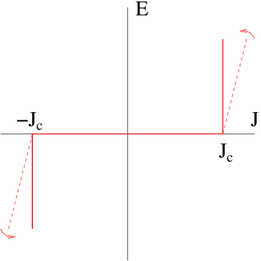
Figure 1: $\{E,J\}$ graph (conduction law) for a hard type-II superconductor, according to Bean’s model. Vertical lines correspond to infinite resistivity above $J_{c}$.

Notice that, if the electric field is nonzero at some point, one has

$${\bf J}=J_{\rm c}{\displaystyle\frac{\bf E}{|{\bf E}|}}$$ (118)

at such point. However, if $E=0$ any value $J\in[-J_{\rm c},J_{\rm c}]$ is allowed. From the physical point of view, the superconductor reacts with a maximal current density flow to the application of electric fields. When the excitation is canceled ($E\to 0$) the flow may remain as a persistent nondissipative current. Notice that the hard superconducting material displays the conventional quasistatic zero resistivity, until a certain level of current transport is demanded ($J_{c}$). Current densities above this threshold are no longer carried by supercharges, and a high electrical resistance is observed.

A fundamental justification of the above model (so-called critical state model), the physical interpretation of the material parameter $J_{\rm c}$ (critical current), and more sophisticated versions may be found in [13, 22, 23] and references therein.

Here, we recall that variational methods are especially useful for solving and generalizing the above statement. To start with, we interpret it as a more realistic limiting process (see figure 1). Thus, the hard material allows lossless subcritical current flow, while it reacts with a high resistivity $E=R(J-J_{\rm c})$ for $J>J_{\rm c}$ (analogously for negative values of $J$). The harder the material, the higher value of $R$, and the more realistic the graph law approximation. Then, one can start with equation (114) and notice that, as $R$ becomes larger, the second term also increases with $J>J_{\rm c}$. In the limit of infinite slope, this fact can be taken into account by reformulating the variational principle as

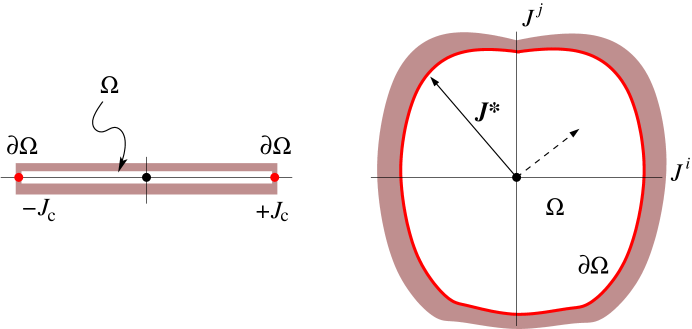
Figure 2: Restriction sets for the current density (${\bf J}\in\Omega$), corresponding to the behavior of hard type-II superconductors. Optimal control solutions obey the condition ${\bf J^{*}}\in\partial\Omega$.

$${\rm min}\quad{\cal S}={\displaystyle\frac{1}{2}\int_{Q}(\Delta{\bf B})^{2}{\,\rm vol}}$$ (119)

$${\rm for\quad|\nabla\times{\bf B}|\leq J_{c}} \,.$$

The inequality (unilateral constraint) determines that the mathematical framework for the model is the so-called Optimal Control Theory [24], an extension of the classical variational calculus for bounded parameter regions. In the Optimal Control language, we have a performance (cost) functional ${\cal S}$ to be minimized under the control equation $\nabla\times{\bf B}={\bf J}$ for bounded parameter $|{\bf J}|\leq J_{c}$. As a very relevant property of this variational interpretation, we remark that the control region for the parameter may be understood as a physically meaningful concept. Thus, one may pose the problem in the very general form

$${\rm min}\quad{\cal S}={\displaystyle\frac{1}{2}\int_{Q}(\Delta{\bf B})^{2}{\,\rm vol}}$$ (120)

$${\rm for\quad\nabla\times{\bf B}\in\Omega} \,,$$

with $\Omega\subset\mathbb{R}^{3}$ some restriction set, prescribed by the underlying physical mechanisms. The conventional statement, given by the graph in figure 1 is nothing but the particular case $\Omega=[-J_{\rm c},J_{\rm c}]$. This is depicted in figure 2. In the literature, several possibilities for the set $\Omega$ have been studied, and identified as the fingerprint of different physical properties. For instance, elliptic restriction sets have been shown to reproduce experimental observations related to anisotropic current flow [25], a rectangular set has been used for producing the so-called double critical state model [26], in which two independent critical current parameters (parallel and normal) are used, etc.

Technical note

The use of the principle (114) as a basis for obtaining (120) deserves some explanation. Not all the hypotheses used in the former case are straightforwardly translated. In particular, one has to recall that the linearization $\Delta{\bf J}=K\cdot{\bf E}$ has to be considered for excursions of $J$ around $J_{c}$. However, according to figure 1, when the electric field is reversed one has $\Delta{J}\simeq 2J_{c}$. Again, the finite jump may be smoothed by taking a small time step. Then, the size of the region where $\Delta{J}=2J_{c}$ is negligible, and the fault has a very small weight in the integral to be minimized.

Finally, we recall that control equations linear in the parameter, as the current case of interest, produce the so-called bang-bang solutions [24], characterized by the condition

$${\bf J^{*}}\in\partial\Omega$$ (121)

i.e. the optimal solutions take values at the boundary of the allowed set. For instance, the control variable jumps between $1$ and $-1$ when $\Omega=[-1,1]$ (see figure 2).

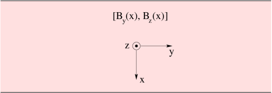
Figure 3: Superconducting slab, subject to magnetic field parallel to the surface.

Example: the infinite slab in parallel field.

The optimal control approach to critical state problems in superconductors has been sometimes misunderstood and qualified as a more or less intuitive approach of restricted applicability. Among other questions, it has been said that it lacks information, because the electric field is absent of the theory. However, this quantity is in the essence of the variational statement, which has been obtained from the general Lagrangian, under the quasi-stationary assumptions (section 4.2). Below, we show with an example that, indeed, the variational statement contains the electric field. Thus, when the minimization process is performed, one obtains the condition that $\bf J$ belongs to the boundary, and also a set of Lagrange multipliers (associated momenta in the Hamiltonian formalism) closely related to the electric field. The comparison of our equations with a more conventional approach that directly uses an ${\bf E}({\bf J})$ relation will prove this aspect.

Let us consider the infinite superconducting slab depicted in figure 3 ($|x|<d/2;|y|,|z|<\infty$), and the problem of determining the electromagnetic response to an excitation field parallel to the surface. Owing to the symmetry, one may use the assumptions

$$\left\{\begin{array}[]{rl}&{\bf B}=(0,B_{y}(x),B_{z}(x))\cr&{\bf J}=(0,J_{y}(x),J_{z}(x))\,.\end{array}\right.$$ (124)

Assuming isotropic conditions, equation (120) takes the form

$${\rm min}\quad{\cal S}={\displaystyle\frac{1}{2}\int_{Q}(\Delta{\bf B})^{2}{\rm vol}}$$ (125)

$${\rm for}\quad J=\;\;\left|{\displaystyle\frac{\partial{\bf B}}{\partial x}}\right|\in\Omega=\left[0,J_{c}\right] \,.$$

Recall that the cost function depends on the field increment $\Delta{\bf B}={\bf B}-{\bf B}_{0}$ for each step of time, in the evolution of the system.

According to Pontryagin’s maximum principle [24], this problem is solved by combination of (i) the canonical equations for the associated Hamiltonian

$${\cal H}={\bf p}\cdot{\displaystyle\Delta{\bf J}}-{\displaystyle\frac{1}{2}(\Delta{\bf B})^{2}}\,,$$ (126)

and (ii) $\Delta{\bf J}^{*}={\bf J}^{*}-{\bf J}_{0}$ such that $H(\Delta{\bf J}^{*})\geq H(\Delta{\bf J})\;,\;\forall\,{\bf J}\in\Omega$, i.e.,

$${\rm max}\left[{\bf p}\cdot{\displaystyle\Delta{\bf J}}\right]\Rightarrow{\displaystyle\frac{\partial{\bf B}}{\partial x}=J_{\rm c}\frac{\bf p}{p}}\,.$$ (127)

This leads to the system

$$\frac{\partial B_{y}}{\partial x} = J_{c}\frac{p_{y}}{p}$$

$$\frac{\partial B_{z}}{\partial x} = J_{c}\frac{p_{z}}{p}$$

$$\frac{\partial p_{y}}{\partial x} = \Delta B_{y}$$

$$\frac{\partial p_{z}}{\partial x} = \Delta B_{z}$$ (128)

By using the definition $(p_{y},p_{z})\equiv\Delta t(E_{z},-E_{y})$ the system may be rewritten as

$$\frac{\partial B_{y}}{\partial x} = J_{c}\frac{E_{z}}{E}$$

$$\frac{\partial B_{z}}{\partial x} = -J_{c}\frac{E_{y}}{E}$$

$$\frac{\partial E_{z}}{\partial x} = \frac{\Delta B_{y}}{\Delta t}$$

$$\frac{\partial E_{y}}{\partial x} = -\frac{\Delta B_{z}}{\Delta t}\,.$$ (129)

Taking derivatives, and inserting the standard notation of dots and primes, one obtains

$$\frac{\partial^{2}B_{y}}{\partial x\partial t} = J_{c}\frac{\dot{E_{z}}E-E_{z}\dot{E}}{E^{2}}$$

$$\frac{\partial^{2}B_{z}}{\partial x\partial t} = -J_{c}\frac{\dot{E_{y}}E-E_{y}\dot{E}}{E^{2}}$$ (130)

and

$$\frac{\partial^{2}B_{y}}{\partial x\partial t} = E_{z}^{\prime\prime}$$

$$\frac{\partial^{2}B_{z}}{\partial x\partial t} = -E_{y}^{\prime\prime}$$ (131)

and thus,

$$E_{z}^{\prime\prime} = J_{c}\frac{\dot{E_{z}}E-E_{z}\dot{E}}{E^{2}}$$

$$E_{y}^{\prime\prime} = J_{c}\frac{\dot{E_{y}}E-E_{y}\dot{E}}{E^{2}}\,.$$ (132)

Now, using polar coordinates in the plain,

$$E_{y}=E\cos{\varphi}$$

$$E_{z}=E\sin{\varphi}$$ (133)

and taking space and time derivatives, it follows

$$E_{z}^{\prime\prime} = E^{\prime\prime}\cos{\varphi}-2E^{\prime}{\varphi}^{\prime}\sin{\varphi}-E(\varphi^{\prime})^{2}\cos{\varphi}-E{\varphi}^{\prime\prime}\sin{\varphi}$$

$$E_{y}^{\prime\prime} = E^{\prime\prime}\sin{\varphi}+2E^{\prime}{\varphi}^{\prime}\cos{\varphi}-E(\varphi^{\prime})^{2}\sin{\varphi}+E{\varphi}^{\prime\prime}\cos{\varphi}$$

$$\dot{E}_{y} = \dot{E}\cos{\varphi}-E\dot{\varphi}\sin{\varphi}$$

$$\dot{E}_{z} = \dot{E}\sin{\varphi}+E\dot{\varphi}\cos{\varphi}\,.$$ (134)

Eventually, back-substitution in equation (4.3) leads to the system

$$\left\{\begin{array}[]{rl}&E^{\prime\prime}=(\varphi^{\prime})^{2}E\cr&2\varphi^{\prime}E^{\prime}+E\varphi^{\prime\prime}=J_{c}\dot{\varphi}\,.\end{array}\right.$$ (137)

These differential equations, together with suitable boundary conditions, allow us to obtain the penetration profiles for the modulus of the electric field and for its angular direction. They have been obtained from our variational approach, and fully coincide with the expressions obtained by the ${\bf E}({\bf J})$ method in reference [27].

5 Conclusions and outlook

In this article, we have shown that the geometric formulation framework of the classical electromagnetic field in terms of differential forms in Minkowski space may be extended to the study of conducting materials.

Related to recent intriguing experimental observations, and to the underlying dissatisfaction caused by a noncovariant theory for several aspects of superconducting electrodynamics, we have proposed a new phenomenological approach to the problem. We show that with the geometric jargon, the theory may be highly simplified. In the language of 1-forms, covariant superconductivity is merely a linear law which admits the inclusion of phenomenological constants and physical quantities. Such quantities allow a direct physical interpretation, as they are a part of wave equations in which they couple to the observable macroscopic fields ${\bf E}$ and ${\bf B}$.

Having clarified the basis of a covariant theory, we also present the complementary side of how covariance should be broken if required by the mathematical counterpart of some physical process. Thus, we show that quasistationary conduction problems may be treated in a spatial 3D covariant framework by pullback of the Minkowski space 1-forms to the $\mathbb{R}^{3}$ Euclidean space. Taking advantage of this prescription, we have been able to justify the use of restricted variational principles in some problems of interest for applied superconductivity.

Two different possibilities for the material law have been considered, ${\cal J}({\cal F})$ and ${\cal J}({\cal A})$, i.e. the current density 1-form either depends on the electromagnetic field 2-form or on the potential 1-form. Being the simplest choice, linear dependencies have been considered.

The linear law ${\cal J}({\cal F})$ is obviously covariant and gauge invariant by construction. However, it is not variational. Only after breaking covariance, and under a quasi-stationary approximation, one can issue a restricted variational principle for such a case. In particular, we obtain an approximated spatial variational statement for linearly dissipating systems (nonconservative forces are proportional to $\partial_{t}{\bf A}$, whose temporal variation may be considered small).

The linear law ${\cal J}({\cal A})$ is covariant and allows a variational statement by endowing the electromagnetic field Lagrangian with an interaction term of the form ${\cal J}\wedge\star{\cal J}$. However, in this case, gauge invariance has to be required. By doing it, one is naturally led to add new currents, generating the equations of superconductivity (${\cal J}=\alpha{\cal A}+\omega$). The most relevant features of this phenomenon are direct consequences of internal symmetries in the field theory. Within the so-called London approximation, the main field is ${\cal A}$. However, the 1-form $\omega$ is required by the theory, coming from an additional field. Outstandingly, this field has observable consequences (as the presence of electrostatic charges and the flux quantization condition), and is sensible to the topology of the material. Just a step further produces the so-called covariant Ginzburg-Landau theory. If one identifies $\omega$ as a Klein-Gordon like probability current density ($\omega\propto\bar{\psi}\,d\psi-\psi\,d\bar{\psi}$), one has a conduction theory with two fields $({\cal A},\psi)$, which may be readily identified as the covariant and gauge invariant generalization of the (non covariant) GL equations of superconductivity. Here $\psi$ represents the wave function of the superconducting carriers.

In the first step, providing the simplest possible covariant expression for the conductivity of a material, we have proposed ${\cal J}=\alpha{\cal A}+\omega$. This fits many experimental observations, including the influence of electrostatic fields on superconductors [7]. However, accounting for other classical [11] and very recent experiments [9], such proposal has been generalized to ${\cal J}=\Xi\,\cdot{\cal A}+\Omega$, with $\Xi$ a $(1,1)$ tensor. This form allows to unify the referred manifestations of superconductivity by either equal or nonequal phenomenological constants in the diagonal terms of $\Xi$. In this sense, when $\Xi$ is nontrivial, we argue that internal symmetries of the charge carriers, and gauge invariance are only compatible through a BCS approach. In this case, an additional field must be introduced, as not only the superconducting carriers are relevant. Nonsuperconducting charges may contribute to the static response of the material and their associated fields could be a matter of further research.

Finally, we stress that the variational interpretation of a priori nonvariational conducting material laws under adiabatic approximation has provided us with a method to treat exotic materials, in which the relation between the fields is well determined through a graph. In particular, this has noticeable consequences in the phenomenological theory of type-II superconductors. We have shown that the so-called Bean’s model for hard type-II superconductors admits a variational formulation, grounded in basic properties of the electromagnetic Lagrangian. This property is of utter importance in the field of applied superconductivity as it allows us to introduce numerical implementations for realistic systems, affected by finite size effects. At the level developed in this work, the material properties are just included by augmenting the basic term ${\cal F}\wedge\star{\cal F}$ with a dissipation function contribution. Extensions of the theory in which the base Lagrangian includes the conservative terms of superconductivity (${\cal J}\wedge\star{\cal J},\;\bar{\bf D}\bar{\Phi}\cdot{\bf D}{\Phi},\dots$) are expeditious.

Variational methods are shown to be equivalent to alternative treatments of the problem, but offer a number of advantages. New mathematical tools, as the optimal control theory, useful for discussing about the existence and form of the electromagnetic problem solution, as well as for hosting numerical implementations, are incorporated.

6 Acknowledgments

The authors acknowledge financial support from Spanish CICYT (Projects BMF-2003-02532 and MAT2005-06279-C03-01).

References

References

- [1] Flanders H 1989 Differential forms with applications to the physical sciences (Mineola, NY: Dover Publications)
- [2] Weinberg S 1996 The Quantum Theory of Fields vol 2 (Cambridge: Cambridge University Press)
- [3] Govaerts J, Bertrand D, Stenuit G 2001 Supercond. Sci. Technol. 14 463
- [4] Govaerts J 2001 J. Phys. A: Math. Gen. 34 8955
- [5] Hirsch J E 2004 Phys. Rev. B 69 214515
- [6] Hirsch J E 2005 Phys. Rev. Lett. 94 187001
- [7] Tao R, Zhang X, Tang X and Anderson P W 1999 Phys. Rev. Lett. 83 5575
- [8] Koyama T 2004 Phys. Rev.B 70 226503; Hirsch J E 2004 Phys. Rev.B 70 226504
- [9] Bertrand D 2005 A Relativistic BCS Theory of Superconductivity: an Experimentally Motivated Study of Electric Fields in Superconductors, Ph D Thesis, Catholic University of Louvain (Louvain-la-Neuve, Belgium); Govaerts J and Bertrand D 2006 arXiv:cond-mat/0608084
- [10] London F and London H 1935 Proc. R. Soc. London 149 71
- [11] London H 1936 Proc. R. Soc. London 155 102
- [12] Zagrodziski J A, Nikiciuk T, Abal’osheva I S and Lewandowski S J 2003 Supercond. Sci. Technol. 16 936
- [13] Badía A and López C 2001 Phys. Rev. Lett. 87 127004
- [14] Crampin M and Pirani F A 1988 Applicable Differential Geometry (Cambridge:Cambridge University Press ).
- [15] Saunders D J The Geometry of Jet Bundles 1989 London Mathematical Society Lecture Notes Series 142. (Cambridge: Cambridge University Press)
- [16] Belinfante J 1939 Physica 6 887
- [17] Itzykson C and Zuber J B 1986 Quantum Field Theory, (New York: McGraw Hill)
- [18] Zhang X H 1989 Phys. Rev. D 39 2933
- [19] Tinkham M 1996 Introduction to Superconductivity 2nd edn (New York: McGraw Hill)
- [20] Goldstein H 1981 Classical Mechanics, 2nd. ed. (Reading MA: Addison-Wesley)
- [21] Bean C P 1964 Rev. Mod. Phys. 36 31
- [22] Bossavit A 1994 IEEE Trans. Magn. 30 3363
- [23] Prigozhin L 1996 Euro. Jnl. of Applied Mathematics 7 237
- [24] Pontryagin L S et al. 1962 The Mathematical Theory of Optimal Processes (New York: Wiley Interscience)
- [25] Badía A and López C 2002 J. Appl. Phys. 92 6110
- [26] Clem J R 1982 Phys. Rev. B 26 2463; Clem J R and Pérez–González A 1984 Phys. Rev. B 30 5041
- [27] Mikitik G P and Brandt E H 2005 Phys. Rev. B 71 012510