Coupled Breathing Oscillations of Two-Component Fermion Condensates
in Deformed Traps

Abstract

We investigate collective excitations coupled with monopole and quadrupole oscillations in two-component fermion condensates in deformed traps. The frequencies of monopole and dipole modes are calculated using Thomas-Fermi theory and the scaling approximation. When the trap is largely deformed, these collective motions are decoupled to the transverse and longitudinal breathing oscillation modes. As the trap approaches becoming spherical, however, they are coupled and show complicated behaviors.

I Introduction

Since the realization of the Bose-Einstein condensed (BEC) atomic gases BECrv ; nobel , there has been much interest in ultracold trapped atomic systems to study quantum many-body phenomena. Besides the Bose-Einstein condensates (BEC) BECrv ; nobel ; bec , one can now study degenerate atomic Fermi gases ferG and bose-fermi mixtures BferM . These systems offer great promise to exhibit new and interesting phenomena of quantum many-particle physics.

Sogo and Yabu SY studied the ground state properties of fermi gas composed by two spin components with various repulsive interaction and showed the phase transition between the paramagnetic and ferromagnetic states. Furthermore we extended this study on the spin phases of the ground state to that for the asymmetric gas with a nets spin in the presence of an external magnetic field and gave the phase diagram about these spin phases ToBe .

An important diagnostic signal for many-body systems is the spectrum of collective excitations. Such oscillations are common to a variety of many-particle systems and are often sensitive to the interaction and the structure of the ground state. In ref.ToBe we have also studied the spin excitation on the dipole and monopole oscillations in the two-component fermion condensed system. The frequencies of the collective oscillations with the out-of-phase show the dependence on the fermion-fermion interaction while those with the in-phase are not sensitive to the interaction. Particularly the frequencies of the out-of-phase modes show rapid changes in the phase transition between the paramagnetic and ferromagnetic spin-phases.

The monopole oscillations can be defined only in the spherical symmetric system. In usual experiments traps have elliptically deformed shapes, where the monopole oscillations are coupled with the quadrupole oscillations. If the trap is largely deformed with the axial symmetry the oscillations must be decoupled into the modes of oscillations along the transverse and longitudinal directions; we shall call them the transverse breathing (TB) and longitudinal breathing (LB) modes.

In this paper we study the coupled oscillation states of the two component fermi gases between the TB and LB modes in deformed traps. The oscillation behaviors are expected to show various features as the deformation of the trap is changed.

The underlying theoretical tool to treat dynamic problems of dilute quantum gases is the time-dependent mean field theory. This is reduced to the random-phase approximation (RPA) for small amplitudes, and the theory in this form has been applied to density oscillations of these systems ClFer ; Kry ; ClSp . When the single-particle spectrum is regular, the long-wavelength excitations are collective and simpler methods can be used to calculate the frequencies, in particular with sum rules sumF or the scaling approximation. In this work we calculate the frequencies of these collective oscillations by using the scaling method scal ; bohi . This scaling method is physically quite transparent, but it is in fact equivalent to the theory based on energy-weighted sum rules bohi , as used for example in ref. sumF .

We will only consider here the case of positive scattering lengths which correspond to a repulsive interaction. When the interaction is attractive, the system is superfluid in its ground state and the excitation properties are controlled by the energy gap. In addition we will focus only on the collective oscillations in the paramagnetic spin phases, and do not deeply discuss those in the ferromagnetic regime.

In the next section we will explain our formulation, and show calculational results in Sec. 3. In Sec.4 we will summarize our work.

II Formalism

We begin with the expression for the energy of a dilute trapped condensate in the mean-field approximation:

$$E_{T} = \int d^{3}r~{}[~{}\frac{\hbar^{2}}{2m}\sum_{s=1,2}\sum_{j=1}^{3}\tau_{s,j}+\frac{m}{2}(\Omega_{T}^{2}r_{1}^{2}+\Omega_{T}^{2}r_{2}^{2}+\Omega_{L}^{2}r_{3}^{2})(\rho_{1}+\rho_{2})+g_{F}\rho_{1}\rho_{2}~{}]$$ (1)

with

$$\tau_{s,j} = \sum_{n}^{occ}\frac{\partial\psi^{*}_{n,s}}{\partial r_{j}}\frac{\partial\psi_{n,s}}{\partial r_{j}}$$ (2)

$$\rho_{s} = \sum_{n}^{occ}\psi^{*}_{n,s}(\mbox{\boldmath$r$})\psi_{n,s}(\mbox{\boldmath$r$}),$$ (3)

where $\psi_{ns}$ are orbital wave functions indexed by orbit $n$ and component $s=1,2$, $\Omega_{L,T}$ are the longitudinal and transverse frequencies of the trapping field and $g_{F}$ is the coupling strength of a contact interaction. Here we assume that all fermions have the same mass, $m$, but we do not need to treat these components as the spin state of the same fermion.

In order to study the collective oscillation, we introduce the following scaling for the fermion wave-function:

$$\psi_{n,s}(\mbox{\boldmath$r$},\tau)=e^{i\xi(\mbox{\boldmath$r$},\tau,s)}e^{\lambda_{T,s}(\tau)+\frac{1}{2}\lambda_{L,s}(\tau)}\psi^{(0)}_{n,s}(e^{\lambda_{T,s}(\tau)}\mbox{\boldmath$r$}_{T};e^{\lambda_{L,s}(\tau)}r_{3}),$$ (4)

with

$$\xi(\mbox{\boldmath$r$},\tau,s)=\frac{\hbar}{m}\left[\frac{1}{2}{\dot{\lambda}}_{T,s}(\tau)\mbox{\boldmath$r$}_{T}^{2}+\frac{1}{2}{\dot{\lambda}}_{L,s}(\tau)r_{3}^{2}\right]$$ (5)

where $\psi_{n,s}^{(0)}$ is the wave-function in the ground state, $\lambda_{T,L}(s)$ are the time-dependent collective coordinates for the oscillation, and ${\dot{\lambda}}_{T,L}(s)$ are the time-derivatives of $\lambda_{T,L}(s)$ . The factor $exp(i\xi)$ is the Gallilei transformation factor which is determined to satisfy the continuum equation.

Let us obtain the total energy under the above scaling by substituting the wave-function (4) into the total energy functional (1). The total energy becomes

$$E_{T} = \frac{\hbar^{2}}{2m}\sum_{s=1,2}\int d^{3}r\left\{(\nabla\xi)^{2}\rho_{s}+e^{2\lambda_{T,s}}(\tau^{(0)}_{s,1}+\tau^{(0)}_{s,2})+e^{2\lambda_{L,s}}\tau^{(0)}_{s,3}\right\}$$ (6)

$$+\frac{1}{2}m^{2}\sum_{s=1,2}\int d^{3}r\left\{e^{-2\lambda_{T,s}}\Omega_{T}^{2}(r_{1}^{2}+r_{2}^{2})+e^{-2\lambda_{L,s}}\Omega_{L}^{2}r_{3}^{2})\right\}\rho_{s}^{(0)}(\mbox{\boldmath$r$}),$$

$$+ge^{2\lambda_{T,1}+\lambda_{L,1}+2\lambda_{T,2}+\lambda_{L,2}}\int d^{3}r~{}\rho_{1}^{(0)}(e^{\lambda_{T,1}}\mbox{\boldmath$r$}_{T};e^{\lambda_{L,1}}r_{3})\rho^{(0)}_{2}(e^{\lambda_{T,2}}\mbox{\boldmath$r$}_{T};e^{\lambda_{L,2}}r_{3})$$

where the superscript $(0)$ indicates $\tau_{s,j}$ and $\rho_{s}$ at the ground state.

In this work we use the Thomas-Fermi (TF) approximation to evaluate the above total energies. The TF approximation makes the spherical symmetric in the momentum distribution at each position and gives the following relation:

$$\tau^{(0)}_{s,1}=\tau^{(0)}_{s,2}=\tau^{(0)}_{s,3}=\frac{1}{10m}(6\pi^{2})^{\frac{2}{3}}{\rho_{s}^{(0)}}^{\frac{5}{3}}.$$ (7)

In addition the ground state densities $\rho^{(0)}_{s}$ become functions of $\Omega_{T}(r_{1}^{2}+r_{2}^{2})+\Omega_{L}r_{3}^{2}$ .

Here we can then make a change of variables to simplify the appearance of the Thomas-Fermi equations as follows.

$$x_{j} = (\frac{m^{2}g_{0}\Omega_{j}}{3\pi^{2}\hbar^{3}})r_{j}~{}~{}~{}~{}~{}(j=1\sim 3),$$

$$n_{s} = \left(\frac{mg_{0}}{\hbar^{2}}\right)^{3}\frac{2}{9\pi^{4}}\rho_{s}^{(0)}~{}~{}~{}~{}~{}(s=1,2),$$

$${\tilde{E}}_{T} = \frac{4m^{12}g_{0}^{8}\Omega_{L}\Omega_{T}^{2}}{(3\pi^{2})^{7}\hbar^{21}}E_{T},$$

$$g = \frac{g_{F}}{g_{0}}$$ (8)

where $g_{0}$ is a certain coupling constant which is chosen later.

With the scaled variables and the Thomas-Fermi approximation, the expression for the total energy at the ground state is

$${\tilde{E}}^{(0)}_{T}=\int d^{3}x~{}\{\sum_{s=1,2}(\frac{3}{5}n_{s}^{\frac{5}{3}}+x^{2}n_{s})+gn_{1}n_{2}\},$$ (9)

where $x^{2}=|\mbox{\boldmath$x$}|^{2}$. The TF equations for the densities $n_{1,2}$ are derived by variation of the energy with a constrain on the fermion numbers. This yields

$$n_{1}^{\frac{2}{3}}+gn_{2} = e_{1}-x^{2}=e_{f}+{\tilde{B}}-x^{2}$$

$$n_{2}^{\frac{2}{3}}+gn_{1} = e_{2}-x^{2}=e_{f}-{\tilde{B}}-x^{2}$$ (10)

In this equation $e_{1}$ and $e_{2}$ are the Lagrange multiplier to constraint the numbers of the fermion-1, $N_{1}$ and -2, $N_{2}$, respectively, and they are rewritten with $e_{f}$ and ${\tilde{B}}$; these $e_{f}$ and ${\tilde{B}}$ have the meanings of the Fermi energy and the external magnetic field in fermion gas when the two components of fermions are described with two different spin states of one fermion.

In this expression the ground state is determined by the three variables, $g$, $e_{f}$ and ${\tilde{B}}$, but the two variables, $g$ and $e_{f}$, are not independent because of the scale symmetry in eq.(10) SY ; ToBe . In this work we choose $g_{0}$ as a critical coupling constant of the paramagnetic and ferromagnetic phase transition at a fixed chemical potential in the symmetric system $\rho_{1}^{(0)}=\rho_{2}^{(0)}$. With this choice the fermi energy is fixed to be $e_{f}=20/27$. The solution of these equations is discussed in detail in ref. ToBe . With fixed values of $e_{f}=20/27$ and ${\tilde{B}}=0$, the spin phase of the two component fermi gas turns to be ’paramagnetic’ ($g<1$) , ’ferromagnetic’($g>1$) in order as the coupling constant, $g$, increases.

Furthermore the total energy in collective oscillations is given as

$${\tilde{E}}_{T} = \frac{1}{2}\sum_{s}{\tilde{X}}_{s}\left\{\frac{2e^{-2\lambda_{T,s}}}{3\omega_{T}^{2}}{\dot{\lambda}}^{2}_{T,s}+\frac{e^{-2\lambda_{L,s}}}{3\omega_{L}^{2}}{\dot{\lambda}}^{2}_{L,s}\right\}$$ (11)

$$+ \sum_{s}\left\{\frac{2e^{2\lambda_{T,s}}+e^{2\lambda_{L,s}}}{3}{\tilde{T}}_{s}+\frac{2e^{-2\lambda_{T,s}}+e^{-2\lambda_{L,s}}}{3}{\tilde{X}}_{s}\right\}+\mbox{${\tilde{V}}$}_{ff}$$

with

$${\tilde{T}}_{s} = \frac{3}{5}\int d^{3}x~{}n_{s}^{\frac{5}{3}}(\mbox{\boldmath$x$})$$

$${\tilde{X}}_{s} = \int d^{3}x~{}x^{2}n_{s}(\mbox{\boldmath$x$})$$ (12)

where $x^{2}=|\mbox{\boldmath$x$}|^{2}$, $\omega_{T}=\Omega_{T}/\Omega_{F}$ and $\omega_{L}=\Omega_{L}/\Omega_{F}$ ($\Omega_{F}\equiv\sqrt{\Omega_{T}^{2}\Omega_{L}}$). The interaction energy $\mbox{${\tilde{V}}$}_{ff}$ appears

$${\tilde{V}}_{ff} = ge^{2\lambda_{T,1}+\lambda_{L,1}+2\lambda_{T,2}+2\lambda_{L,2}}\int d^{3}r~{}n_{1}(e^{\lambda_{T,1}}\mbox{\boldmath$x$}_{T},e^{\lambda_{L,1}}x_{3})n_{2}(e^{\lambda_{T,2}}\mbox{\boldmath$x$}_{T},e^{\lambda_{L,2}}x_{3})$$ (13)

In order to describe the collective oscillations, we obtain the variation of the total energy up to the order of $O(\lambda^{2}$) as

$$\Delta E_{T}\equiv E_{T}-E^{(0)}_{T}\approx\frac{1}{2}\mbox{\boldmath${}^{t}{\dot{\lambda}}$}B\mbox{\boldmath${\dot{\lambda}}$}+\frac{1}{2}\mbox{\boldmath${}^{t}\lambda$}C\mbox{\boldmath$\lambda$}$$ (14)

with

$$B=\left(\begin{array}[]{cccc}\frac{4\mbox{${\tilde{X}}$}_{1}}{3\omega_{T}^{2}}&0&0&0\\ 0&\frac{2\mbox{${\tilde{X}}$}_{1}}{3\omega_{L}^{2}}&0&0\\ 0&0&\frac{4\mbox{${\tilde{X}}$}_{2}}{3\omega_{T}^{2}}&0\\ 0&0&0&\frac{2\mbox{${\tilde{X}}$}_{2}}{3\omega_{L}^{2}}\\ \end{array}\right)$$ (15)

$$C = \left(\begin{array}[]{cccc}\frac{8}{3}(\mbox{${\tilde{T}}$}_{1}+\mbox{${\tilde{X}}$}_{1})&0&0&0\\ 0&\frac{4}{3}(\mbox{${\tilde{T}}$}_{1}+\mbox{${\tilde{X}}$}_{1})&0&0\\ 0&0&\frac{8}{3}(\mbox{${\tilde{T}}$}_{2}+\mbox{${\tilde{X}}$}_{2})&0\\ 0&0&0&\frac{4}{3}(\mbox{${\tilde{T}}$}_{2}+\mbox{${\tilde{X}}$}_{2})\\ \end{array}\right)$$ (25)

$$~{}~{}~{}~{}~{}~{}~{}~{}~{}~{}~{}+\left(\begin{array}[]{cccc}~{}-\frac{4}{3}V_{1}-\frac{8}{15}V_{3}{}&~{}-\frac{2}{3}V_{1}-\frac{2}{15}V_{3}{}&~{}\frac{8}{15}V_{3}&\frac{2}{15}V_{3}{}\\ ~{}-\frac{2}{3}V_{1}-\frac{2}{15}V_{3}{}&~{}-\frac{1}{3}V_{1}-\frac{1}{5}V_{3}{}&~{}\frac{2}{15}V_{3}{}&\frac{1}{5}V_{3}{}\\ ~{}\frac{8}{15}V_{3}{}&~{}\frac{2}{15}V_{3}{}&~{}-\frac{4}{3}V_{2}-\frac{8}{15}V_{3}{}&~{}-\frac{2}{3}V_{2}-\frac{2}{15}V_{3}{}\\ ~{}\frac{2}{15}V_{3}&\frac{1}{5}V_{3}{}&~{}-\frac{2}{3}V_{2}-\frac{2}{15}V_{3}{}&-\frac{1}{3}V_{2}-\frac{1}{5}V_{3}\\ \end{array}\right)$$

with

$$V_{1} = g\int d^{3}x~{}\left(xn_{1}\frac{\partial n_{2}}{\partial x}\right),$$ (26)

$$V_{2} = g\int d^{3}x~{}\left(x\frac{\partial n_{1}}{\partial x}n_{2}\right),$$ (27)

$$V_{3} = g\int d^{3}x~{}\left(x^{2}\frac{\partial n_{1}}{\partial x}\frac{\partial n_{2}}{\partial x}\right),$$ (28)

where the vector $\lambda$ is defined as $\mbox{\boldmath${}^{t}\lambda$}=(\lambda_{T,1},\lambda_{L,1},\lambda_{T,2},\lambda_{L,2})$. The terms propritional to $\lambda$ disappears because of the virial theorem.

Then the classical equation of motion for $\lambda$ is harmonic, giving rise to the following eigenvalue equation for the oscillation frequencies,

$$\left[B\omega^{2}-C\right]\mbox{\boldmath$\lambda$}=0.$$ (29)

Before performing actual calculations, we should discuss the collective oscillations in some extreme conditions.

In the largely deformed system, $\omega_{L}>>1$ or $\omega_{T}>>1$, first, the four oscillation modes are decoupled into two groups, two oscillations modes in the longitudinal directions, and the other two modes in the transverse directions. We can obtain these decoupled modes by taking $C_{12}=C_{14}=C_{23}=C_{34}=0$. In the symmetric system, $n_{1}=n_{2}$, furthermore, the two kinds of modes are further decoupled into the in-phase ($\lambda_{L(T),1}=\lambda_{L(T),2}$) and the out-of-phase ($\lambda_{L(T),1}=-\lambda_{L(T),2}$) modes; namely the four excited oscillations are decoupled into the in-phase transverse breathing (ITB), in-phase longitudinal breathing (ILB), out-of-phase transverse breathing (OTB) and out-of-phase longitudinal breathing (OLB) modes.

The oscillation frequencies in the symmetric system become

$${\omega_{T}^{in}}^{2}=\frac{2(\mbox{${\tilde{T}}$}_{1}+\mbox{${\tilde{X}}$}_{1})-V_{1}}{\mbox{${\tilde{X}}$}_{1}}\omega_{T}^{2} ,~{}~{} {\omega_{T}^{out}}^{2}=\frac{2(\mbox{${\tilde{T}}$}_{1}+\mbox{${\tilde{X}}$}_{1})-V_{1}-\frac{4}{5}V_{3}}{\mbox{${\tilde{X}}$}_{1}}\omega_{T}^{2},$$ (30)

$${\omega_{L}^{in}}^{2}=\frac{2(\mbox{${\tilde{T}}$}_{1}+\mbox{${\tilde{X}}$}_{1})-\frac{1}{2}V_{1}}{\mbox{${\tilde{X}}$}_{1}}\omega_{L}^{2} ,~{}~{} {\omega_{L}^{out}}^{2}=\frac{2(\mbox{${\tilde{T}}$}_{1}+\mbox{${\tilde{X}}$}_{1})-\frac{1}{2}V_{1}-\frac{3}{5}V_{3}}{\mbox{${\tilde{X}}$}_{1}}\omega_{L}^{2},$$ (31)

where the superscripts ’$in$’ and ’$out$’ indicate the in-phase and out-of-phase modes, respectively, and the subscripts ’T’ and ’L’ denote the oscillations in the transverse and longitudinal directions, respectively. Note that $\mbox{${\tilde{T}}$}_{1}=\mbox{${\tilde{T}}$}_{2}$, $\mbox{${\tilde{X}}$}_{1}=\mbox{${\tilde{X}}$}_{2}$ and so on.

Next we discuss the oscillations in the near-spherical symmetric system, $\omega_{L}\approx\omega_{T}\approx 1$. In this system the oscillation modes are decoupled into the monopole and quadrupole oscillation modes.

By taking the collective coordinates to be $\lambda_{L,i}=\lambda_{T,1}=\lambda_{i}$ , we can obtain the frequencies of the monopole oscillations with the following equation:

$$\left[\left(\begin{array}[]{cc}2\mbox{${\tilde{X}}$}_{1}&0\\ 0&2\mbox{${\tilde{X}}$}_{2}\end{array}\right)\frac{\omega_{2}}{\Omega_{M}^{2}}-\left(\begin{array}[]{cc}4(\mbox{${\tilde{T}}$}_{1}+\mbox{${\tilde{X}}$}_{1})-3V_{1}-V_{3}&V_{3}\\ V_{3}&4(\mbox{${\tilde{T}}$}_{2}+\mbox{${\tilde{X}}$}_{2})-3V_{2}-V_{3}\end{array}\right)\right]\left(\begin{array}[]{c}\lambda_{1}\\ \lambda_{2}\end{array}\right)=0$$ (32)

with

$$\frac{1}{\Omega_{M}^{2}}=\frac{1}{3}(\frac{2}{\omega_{T}^{2}}+\frac{1}{\omega_{L}^{2}}).$$ (33)

By taking the collective coordinates to be $\lambda_{T,i}=-\lambda_{L,i}/2=\lambda_{i}$, similarly, we can also calculate the frequencies of the quadrupole oscillations with

$$\left[\left(\begin{array}[]{cc}\mbox{${\tilde{X}}$}_{1}&0\\ 0&\mbox{${\tilde{X}}$}_{2}\end{array}\right)\frac{\omega^{2}}{\Omega^{2}_{Q}}-\left(\begin{array}[]{cc}2(\mbox{${\tilde{T}}$}_{1}+\mbox{${\tilde{X}}$}_{1})-\frac{1}{5}V_{3}{}&\frac{1}{5}V_{3}{}\\ \frac{1}{5}V_{3}{}&2(\mbox{${\tilde{T}}$}_{2}+\mbox{${\tilde{X}}$}_{2})-\frac{1}{5}V_{3}\end{array}\right)\right]\left(\begin{array}[]{c}\lambda_{1}\\ \lambda_{2}\end{array}\right)=0$$ (34)

with

$$\frac{1}{\Omega_{Q}^{2}}=\frac{1}{3}(\frac{1}{\omega_{T}^{2}}+\frac{2}{\omega_{L}^{2}}).$$ (35)

In the symmetric system $\rho_{1}^{(0)}=\rho_{2}^{(0)}$, these modes are also decoupled to the in-phase and the out-of-phase modes. Then the oscillation frequencies in the symmetric system become

$${\omega_{M}^{in}}^{2}=\frac{2(\mbox{${\tilde{T}}$}_{1}+\mbox{${\tilde{X}}$}_{1})-\frac{3}{2}V_{1}}{\mbox{${\tilde{X}}$}_{1}}\Omega_{M}^{2}, {\omega_{M}^{out}}^{2}=\frac{2(\mbox{${\tilde{T}}$}_{1}+\mbox{${\tilde{X}}$}_{1})-\frac{3}{2}V_{1}-V_{3}}{\mbox{${\tilde{X}}$}_{1}}\Omega_{M}^{2}.$$ (36)

$${\omega_{Q}^{in}}^{2}=\frac{2(\mbox{${\tilde{T}}$}_{1}+\mbox{${\tilde{X}}$}_{1})}{\mbox{${\tilde{X}}$}_{1}}\Omega_{Q}^{2}, {\omega_{Q}^{out}}^{2}=\frac{2(\mbox{${\tilde{T}}$}_{1}+\mbox{${\tilde{X}}$}_{1})-\frac{2}{5}V_{3}}{\mbox{${\tilde{X}}$}_{1}}\Omega^{2}.$$ (37)

where the subscript ’M’ and ’Q’ indicate the monopole and quadrupole frequencies, respectively.

III Results

In this section we discuss the collective oscillations coupled with the transverse and longitudinal breathing modes. As mentioned in the previous section we fix the fermi energy to be $e_{f}=20/27$, which makes the parametric and ferromagnetic spin phase transition at $g=1$ when ${\tilde{B}}=0$.

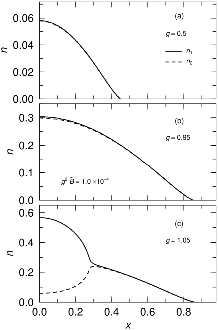
Figure 1: The scaled density distribution of two components fermion at $g=0.5$ (a), $g=0.95$ (b) and $g=1.05$ (c) with with $e_{f}=20/27$ and $g^{2}{\tilde{B}}=1.0\times 10^{-4}$. The solid and dashed lines represents the distribution of the major and minor components, respectively.

Density profiles illustrating these three regimes are shown in Fig. 1. The panels show the densities as a function of distance $x$ in a weak magnetic field ($g^{2}\mbox{${\tilde{N}}_{B}$}=1.0\times 10^{-4}$) and at three different interaction strengths: $g=0.5$(a), 0.95(b) and 1.05(c). The solid and dashed lines represent the scaled density distribution of major and minor components of fermions. From top to bottom, the panels show paramagnetic (a,b) and ferromagnetic (c).

Next we calculate the collective oscillations by solving eigenvalue equation (29). In this equation we obtain four eigenvalues corresponding to collective oscillation frequencies. For convenience we define these four frequencies as $\omega_{1}$, $\omega_{2}$, $\omega_{3}$ and $\omega_{4}$ in order of the frequencies from the larger one to the lower one. In addition we refer to the four collective modes with the frequencies $\omega_{1}$, $\omega_{2}$, $\omega_{3}$ and $\omega_{4}$ as modes-1, -2, -3 and -4, respectively.

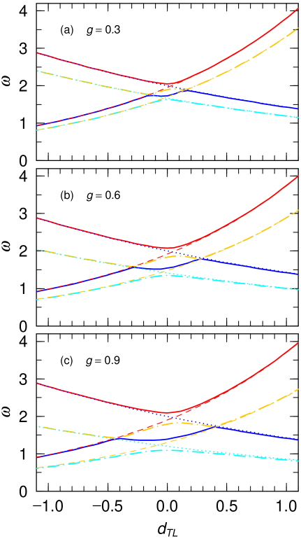
Figure 2: The frequencies of the collective oscillations versus $\omega_{L}/\omega_{T}$ at $g=0.3$ (a), $g=0.6$ (b) and $g=0.9$ (c) with $e_{f}=20/27$ and $g^{2}{\tilde{B}}=1.0\times 10^{-4}$. The solid lines represent the results with the full calculations, and the dashed and dotted lines indicate the frequencies of the transverse and longitudinal breathing modes, respectively.

In Fig. 2 we show the frequencies of oscillations as functions of the deformation parameter $d_{TL}=\ln(\omega_{L}/\omega_{T})$ at the coupling constant $g=0.3$ (a), $=0.6$ (b) and $=0.9$ (c). The solid lines represent the first and third frequencies $\omega_{1}$ and $\omega_{3}$, and the chain-dotted lines indicate $\omega_{2}$ and $\omega_{4}$. In these calculation we take the magnetic field to be $g^{2}{\tilde{B}}=1.0\times 10^{-4}$, where the system is almost symmetric between the two component, $N_{1}\approx N_{2}$. In the same figures, furthermore, we also plot the frequencies of the transverse and longitudinal breathing modes with the dashed and dotted lines, respectively.

First we see the strong level mixing between modes-2 and -3 at two deformation parameters, $d_{TL}=d_{1}$ and $d_{2}$ ($d_{1}<0<d_{2}$). When $d_{TL}<d_{1}$ and $d_{2}<d_{TL}$, the frequencies in the full calculation (solid lines) are almost the same as those in the calculations decoupled with the transverse and longitudinal modes (dashed and dotted lines), though they are quite different when $d_{1}<d_{TL}<d_{2}$.

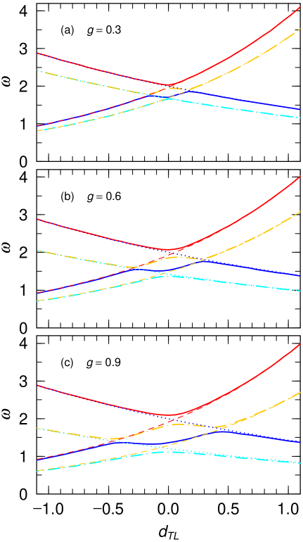
Figure 3: Same as Fig. 2, but with $g^{2}{\tilde{B}}=1.0\times 10^{-2}$.

In Fig. 3 we also give the same quantities but with $g^{2}{\tilde{B}}=1.0\times 10^{-2}$. The system is not symmetric $n_{1}\neq n_{2}$, but the results are quite similar to those in Fig. 2 though the difference in the frequency at the level mixing points between the modes-2 and -3 is a little larger than those in Fig. 2.

For future discussions we refer to the three deformation parameter regions, $d_{TL}<d_{1}$, $d_{1}<d_{TL}<d_{2}$ and $d_{2}<d_{TL}$ as the prolate deformed, the semi-spherical and the prolate deformed regions, respectively. The transverse and longitudinal breathing oscillation modes are almost decoupled in both the oblate and prolate deformed regions, while these modes are coupled in the spherical region.

In order to know the level mixing behaviors more, we calculate the four following components:

$$\lambda_{T}^{in}=\frac{1}{\sqrt{2}}(\lambda_{T,1}+\lambda_{T,2}), \lambda_{L}^{in}=\frac{1}{\sqrt{2}}(\lambda_{L,1}+\lambda_{L,2}),$$ (38)

$$\lambda_{T}^{out}=\frac{1}{\sqrt{2}}(\lambda_{T,1}-\lambda_{T,2}), \lambda_{L}^{out}=\frac{1}{\sqrt{2}}(\lambda_{L,1}-\lambda_{L,2}),$$ (39)

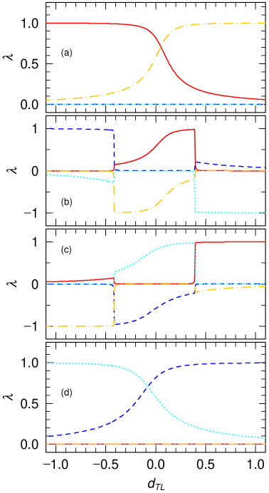
Figure 4: Components of the eigenvectors of mode-1 (a), mode-2 (b), mode-3 (c) and mode-4 (d) at $g=0.9$ with $g^{2}{\tilde{B}}=1.0\times 10^{-4}$. The solid and chain-dotted lines represent the in-phase transverse and longitudinal components, respectively, and the dashed and dotted lines denote the out-of-phase transverse and longitudinal components, respectively.

where $\lambda_{T}^{in}$, $\lambda_{L}^{in}$, $\lambda_{T}^{out}$ and $\lambda_{L}^{out}$ are components of the ITB, ILB, OTB and OLB modes, respectively. In Fig. 4 we show the components of the eigenvectors at the mode-1 (a), the mode-2 (b), the mode-3 (c) and the mode-4 (d) with $g=0.9$ and $g^{2}{\tilde{B}}=1.0\times 10^{-4}$. The solid, chain-dotted, dashed and dotted lines represent $\lambda_{T}^{in}$, $\lambda_{L}^{in}$, $\lambda_{T}^{out}$ and $\lambda_{L}^{out}$, respectively.

The results show that the phase of the modes-1 and -4 are in-phase in all $d_{TL}$ regime. When the system is oblate deformed ($d_{TL}<<0$). the mode-1 is almost the ITB mode. As $d_{TL}$ increase, the system approaches the spherical, the ILB component in the mode-1 mode gradually becomes larger. When the system becomes spherical ($d_{TL}=0$), the mode-1 becomes a mixed mode with the ITB and ILB in the same ratio: namely the mode-1 is the monopole oscillation. As the system is further deformed to the prolate shape, the transverse component decreases and the longitudinal one increases and the oscillation becomes the in-phase longitudinal oscillation in $\omega_{L}/\omega_{T}\rightarrow\infty$ limit.

The mode-4 has the same behavior, but its phase is out-of-phase; the OTB mode when $d_{TL}<d_{1}$, the out-of-phase monopole mode at $d_{TL}=0$ and the OLB mode when $d_{TL}>d_{2}$.

The variations of the modes-2 and -3 show more complicated behaviors. The mode-2 is mainly the OTB mode in the oblate deformed region ($d_{TL}<d_{1}$), and the OLB mode in the prolate deformation region ( $d_{TL}>d_{2}$). The mode-3 is the ILB mode in the oblate deformation, and the ITB mode in the prolate deformation. At $d_{TL}=d_{1}$ and $d_{2}$, the modes-2 and -3 make the level mixing and exchange their roles. Namely the modes-2 and -3 are in-phase out-of-phase oscillations in the semi-spherical region, respectively. As $d_{TL}$ approaches zero, the TB and LB oscillation modes are mixed. At $d_{TL}=0$, the mode-2 becomes the in-phase quadrupole oscillations, ($\lambda_{L}^{in}=-2\lambda_{T}^{in}$) and the mode-3 becomes the out-of-phase ones, respectively.

Thus we know that the four modes agree with the frequencies of the TB and LB modes, when $\omega_{L}/\omega_{T}>>1$ ($d_{TL}>>0$), and $\omega_{T}/\omega_{L}>>1$ ($d_{TL}<<0$). On the other hand these modes show different behaviors in the nearly spherical symmetric system ($d_{TL}\approx 0$), where the collective oscillations are described as the coupled modes of the monopole and quadrupole oscillations.

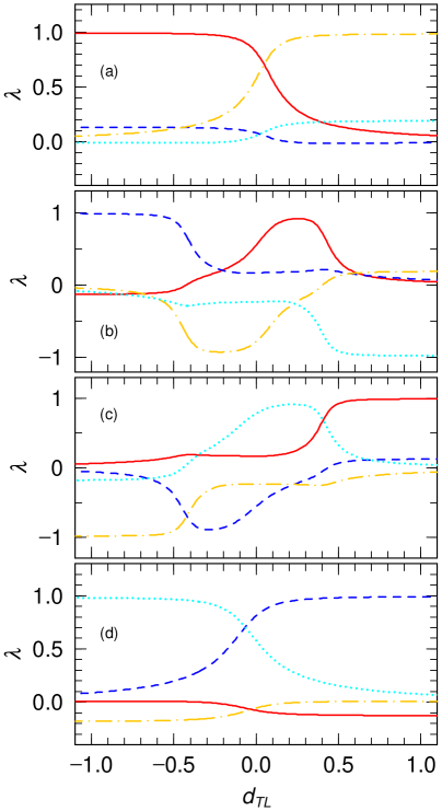
Figure 5: Same as Fig. 4, but with $g^{2}{\tilde{B}}=1.0\times 10^{-2}$.

In Fig. 5, furthermore, we show the same quantities in Fig. 4 but with $g^{2}{\tilde{B}}=1.0\times 10^{-2}$. The feature discussed above is less clear, but also seen in the case of the strong magnetic field.

When $g^{2}{\tilde{B}}=1.0\times 10^{-2}$, the number asymmetry is not so small, $N_{1}\gtrsim N_{2}$. The mixing between the in-phase and out-of-phase modes is very small in modes-1 and -4. The similar result was shown for the monopole oscillation in the spherical trap. Even in modes-2 and -3, this mixing is seen only in the region near $d_{TL}\approx d_{1}$ and $d_{TL}\approx d_{2}$. Hence we can disregard the mixing between the in-phase and out-of-phase modes in qualitative discussions, and consider that modes-2 and -3 exchange their roles around $d_{TL}\approx d_{1}$ and $d_{TL}\approx d_{2}$.

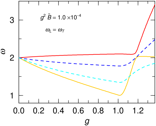
Figure 6: The frequency of the monopole and quadrupole oscillations with the external magnetic fields with $g^{2}{\tilde{B}}=$ $1.0\times 10^{-4}$. The solid and dashed lines represent the results of the monopole and quadrupoles modes, respectively.

In order to know more details of the deformation dependence, we should examine relations between the frequencies of the collective oscillations and the coupling constant $g$. First we show the frequencies of the monopole and quadrupole oscillations versus the coupling constant $g$ in the spherical symmetric system ($\omega_{L}=\omega_{T}$) with the $g^{2}{\tilde{B}}=1.0\times 10^{-4}$ in Fig. 6. The solid and dashed lines represent the results of the monopole and quadrupole oscillations. In the completely spherical symmetric system the monopole and quadrupole states are decoupled, and there is no level mixing between these two modes. In the paramagnetic phase ($g\lesssim 1.0$), larger frequencies correspond to the in-phase oscillation modes both in the monopole and quadrupole modes. The monopole modes make the level mixing between the in-phase and out-of-phase modes in the ferromagnetic phase ($g\lesssim 1.0$), while the quadrupole modes do not show the level mixing. As the coupling becomes larger, the frequency of the oscillation modes except the in-phase monopole oscillation mode decreases monotonically until $g\approx 1.0$, and increases above that, while the frequencies of the in-phase monopole oscillation are almost invalid. When the coupling constant increases further, the level mixing between the two modes of the monopole oscillation occurs.

Next we study the non-symmetric system, where all the four modes can be mixed. In Fig. 7 we show the frequencies of the mode-1, -2, -3 and -4 as the functions of the coupling constant with $\omega_{L}/\omega_{T}=1.5$ ($d_{TL}=0.41$) (a), $\omega_{L}/\omega_{T}=0.7$ ($d_{TL}=-0.36$) (b), $\omega_{L}/\omega_{T}=0.5$ ($d_{TL}=-0.69$) (c) and $\omega_{L}/\omega_{T}=0.3$ ($d_{TL}=-1.2$) (d). In these figures we see again that the levels between modes-2 and -3 are mixed at a certain $g$. When $\omega_{L}/\omega_{T}=0.7$ (Fig. 7), for example, the frequencies of modes-1 and -2 are $\omega=2\omega_{T}$, and those of modes-3 and -4 are $\omega=2\omega_{L}$ at $g=0$. As the coupling becomes larger, the frequencies of modes-2 and -4 monotonously decreases while those of modes-1 and -3 is almost invalid, and then the the level mixing between modes-2 and -3 occurs at $g\approx 0.37$.

As the deformation parameter $d_{TL}$ increases, the difference between $\omega_{T}$ and $\omega_{L}$ becomes larger, and the level mixing occurs at larger coupling constant. As the deformation parameter further increases, the level mixing disappears when $d_{TL}<d_{1}$ because the minimum value of $\omega_{2}$ is larger than $\omega_{3}$, and the level mixing cannot occur. The $\omega_{2}$ becomes minimum at the border between the paramagnetic and ferromagnetic phases $g\approx 1$, where the level mixing occurs when $d_{TL}=d_{1}$.

In Fig. 8 we show the components of the eigenvectors at the mode-1 (a), the mode-2 (b), the mode-3 (c) and the mode-4 (d) with $g^{2}{\tilde{B}}=1.0\times 10^{-4}$ and $\omega_{L}/\omega_{T}=0.7$. The mode-1 and the mode-4 are almost ITB and OLB modes in the weak coupling region, respectively. As the coupling, $g$, increases, the ILB and OTB components are gradually mixed in both the modes. In the case of the mode-1, this mixing is small, while in the mode-4 the OLB and OTB components are more largely mixed, particularly around $g\approx 1$.

In this figure, furthermore, we can also see the level mixing between modes-2 and -3. At $g=0$ the mode-2 and the mode-3 are the ILB and OTB modes. As the coupling increases, the ITB and OLB components are more mixed in the mode-2 and the mode-3, respectively. At $g\approx 0.37$ the level mixing occurs. The strength of the components is exchanged between the modes-2 and -3.

IV Summary

In this paper we study the collective breathing oscillations in the deformed traps. The oscillations contain the four kinds of the oscillation, ITB, OTB, ILB and OLB modes. When the shape of the traps are largely deformed, either oblate or prolate, these modes are decoupled. As this shape becomes close to being spherical, the transverse and longitudinal modes are coupled, and make the monopole and quadrupole oscillations. The borders between these coupling and decoupling are at $d_{TL}\approx d_{1}$ and $d_{TL}\approx d_{2}$, where the OTB and ILB modes make level crossing.

In the deformed traps the frequencies of the ITB and ILB modes agree with twice of the trap frequencies and are not so different from those of the non-interacting system. The frequencies of the OTB and OLB modes show some coupling dependence and give information of the interaction, Their qualitative behaviors are however similar to those in the dipole oscillation ToBe .

In the semi-spherical traps, on the other hand, the collective oscillations exhibit more complicated behavior because of the level mixing. Hence we can get significant information on many body system of fermi gas by investigate breathing oscillations with the various fermion-fermion couplings and deformations of the trap near being spherical ($0.4\lesssim\omega_{L}/\omega_{T}\lesssim 1.6$).

In this work we do not discuss extremely deformed system ($\omega_{T}\rightarrow\infty$ or $\omega_{L}\rightarrow\infty$). In such extreme conditions the system becomes a quasi-low dimension one Petrov , and the collective oscillation can be expected to show quite different behaviors from those in our work Nishimura1 .

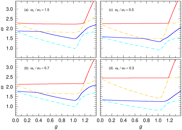
Figure 7: The frequencies of the collective oscillations versus the coupling constant $g$ with the external magnetic fields with $g^{2}{\tilde{B}}=$ $1.0\times 10^{-4}$ for $\omega_{L}/\omega_{T}=1.5$ (a), 0.7 (b), 0.5 (c) and 0.3 (b). The solid lines represent the results of the mode-1 and the mode-3, and the chain-dotted lines indicate those of the mode-2 and the mode-4.

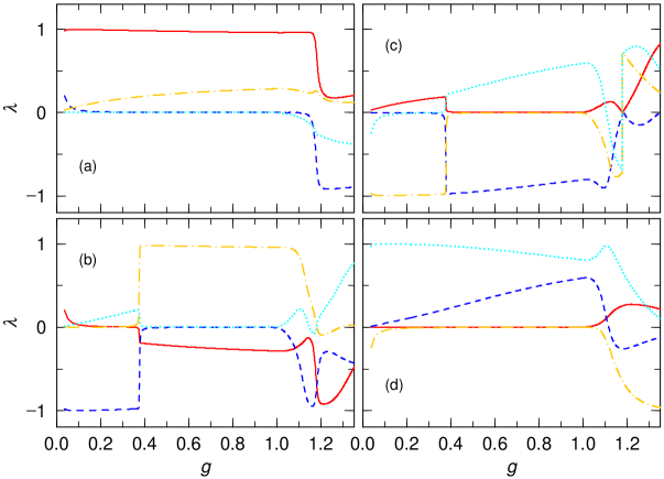
Figure 8: Components of the eigenvectors of mode-1 (a), mode-2 (b), mode-3 (c) and mode-4 (d) with $g^{2}{\tilde{B}}=1.0\times 10^{-4}$ and $\omega_{L}/\omega_{T}=0.7$. The solid and chain-dotted lines represent the in-phase transverse and longitudinal components, respectively, and the dashed and dotted lines denote the out-of-phase transverse and longitudinal components, respectively.

References

-
(1)
For reviews, see: A.S. Parkins and H.D.F. Walls,
Phys. Rep. 303, 1 (1998);
F. Dalfovo, S. Giorgini, L.P. Pitaevskii and S. Stringari,
Rev. Mod. Phys. 71, 463 (1999);
W. Ketterle, D.S. Durfee, and D.M Stamper-Kum, in Bose-Einstein Condensation in Atomic Gases Proc. of Internationa School of Physic ”Enrico Fermi”, edited by M. Ingusico, S. Stringari and C. Wieman (IOS Press, Amsterdam, 1999) -
(2)
E.A. Cornell and C.E. Wieman, Rev. Mod. Phys. 74, 875 (2002);
W. Ketterle, Rev. Mod. Phys. 74, 1131 (2002). -
(3)
M. H. Anderson, et al.
Science 269, 198 (1995);
K. B. Davis, et al., Phys. Rev. Lett. 75, 3969 (1995). -
(4)
B. DeMarco and D.S. Jin, Science 285, 1703 (1999);
S.R. Granade, et al., Phys. Rev. Lett. 88, 120405 (2002). -
(5)
A.G. Tuscott, K.E. Strecker, W.I. McAlexander, G.B. Parridge, and
R.G. Hullet, Science 291, 2570 (2001);
F. Schreck, et al., Phys. Rev. Lett. 87, 080403 (2001);
Z. Hadzibabic, et al., Phys. Rev. Lett. 88, 160401 (2002); 91, 160401 (2003) ;
T. Maruyama, H. Yabu and T. Suzuki, Phys. Rev. A72, 013609 (2005). - (6) T. Sogo and H. Yabu, Phys. Rev. A66, 043611 (2002)
- (7) T. Maruyama and G.F. Bertsch, Phys. Rev. A 73, 013610 (2006).
- (8) G.M. Bruun, Phys. Rev. A63, 043408 (2001).
- (9) Kryzysztof Goral, Miro, Phys. Rev. A67, 025601 (2003).
- (10) G.M. Bruun and B.R. Mottelson, Phys. Rev. Lett 87, 270403 (2001).
- (11) L. Vichi and S. Stringari, Phys. Rev. A60, 4734 (1999).
-
(12)
G.F. Bertsch, Nucl. Phys. A249, 253 (1975) ;
G.F. Bertsch and K. Stricker, Phys. Rev. C13, 1312 (1976);
D.M. Brink and Leobardi, Nucl. Phys. A258, 285 (1976);
T. Suzuki, Prog. Theor. Phys. 64, 1627 (1980). - (13) O. Bohigas, A.M. Lane and J. Martorell, Phys. Rep. 51, 267 (1979),
- (14) D.S. Petrov, D.M.Gangardt and G.V.Shlyapnikov, J. Phys. IV France 116, 3 (2006).
- (15) S. Nishimura and T. Maruyama, in preparation.