Electron spin as a spectrometer of nuclear spin noise and other fluctuations

1 Introduction

Although the study of electron spin dynamics using pulse electron spin resonance is an established research field schweiger01 , many theoretical questions regarding the microscopic mechanisms for reversible and irreversible decay of spin coherence remain open. Recently, the quest towards scalable quantum computation using electron spins hu04 gave new impetus to pulse spin resonance, and sparked major experimental progress towards control and detection of individual electron spins in the solid state environment jelezko04 ; elzerman04 ; xiao04 ; rugar04 ; petta05 .

The microscopic understanding of the mechanisms leading to electron spin energy and phase relaxation, and the question of how to control these processes is central to the research effort in spin-based quantum computation. The goal of theory is to achieve microscopic understanding so that spin coherence can be controlled either from a materials perspective (i.e., choosing the best nanostructure for spin manipulation and dynamics) or from the design of efficient pulse sequences that reach substantial coherence enhancement without a high overhead in number of pulses and energy deposition. (The latter is particularly important in the context of low temperature experiments where undesired heating from the microwave excitations must be avoided).

One has to be careful in order to distinguish the time scales characterizing electron spin coherence. It is customary to introduce three time scales, $T_{1}$, $T_{2}^{*}$, and $T_{2}$. For localized electron spins, these time scales usually differ by many orders of magnitude, because each is dominated by a different physical process. $T_{1}$ is the $1/e$ decay time for the spin magnetization along the external magnetic field direction. As an example, $T_{1}$ of a phosphorus donor impurity in silicon is of the order of a thousand seconds at low temperatures and moderate magnetic fields ($T=4$ K and $B=0.3$ T) feher59b . These long $T_{1}$’s are explained by noting that the spin-orbit interaction produces a small admixture of spin up/down states; the electron-phonon interaction couples these admixtures leading to $\frac{1}{T_{1}}\propto B^{5}$ at low temperatures haseg_roth60 ; desousa03c . $T_{1}$ is generally long because a spin-flip in a magnetic field requires energy exchange with the lattice via phonon emission. The time scales $T_{2}^{*}$ and $T_{2}$ are instead related to phase relaxation, and hence do not require transmission of energy to the lattice. Here $T_{2}^{*}$ is the 1/e decay time of the precessing magnetization in a free induction decay (FID) experiment ($\pi/2-t-\rm{measure}$, where $\pi/2$ denotes a spin rotation around the $x$ axis). Hence $T_{2}^{*}$ is the decay time of the total in-plane magnetization of an ensemble of spins separated in space or time (e.g., a group of impurities separated in space, or the time-averaged magnetization of a single spin, as discussed in section 2.3 below). For a phosphorus impurity in natural silicon, $T_{2}^{*}\approx~{}20$ ns due to the distribution of frozen hyperfine fields, that are time-independent within the measurement window of the experiment. The $T_{2}^{*}$ decay is reversible, because the ensemble in-plane magnetization is almost completely recovered by applying a spin-echo pulse sequence. In this review we define $T_{2}$ as the 1/e decay time of a Hahn echo ($\pi/2-\tau-\pi-\tau-\rm{echo}$). The irreversible decoherence time $T_{2}$ is caused by uncontrolled time dependent fluctuations within each time interval $\tau$. For a phosphorus impurity in natural silicon, we have $T_{2}\approx 0.3$ ms chiba72 , four orders of magnitude longer than $T_{2}^{*}$.

The discussion above clearly indicates that the resulting coherence times are critically dependent on the particular pulse sequence chosen to probe spin dynamics. In section 2 we show that spin coherence can be directly related to the spectrum of electron spin phase fluctuations and a filter function appropriate for the particular pulse sequence. The phase of a precessing electron spin is a sensitive probe of magnetic fluctuations. This gives us the opportunity to turn the problem around and view pulse electron spin resonance as a powerful tool enabling the study of low frequency magnetic fluctuations arising from complex many-body spin dynamics in the environment surrounding the electron spin.

A particularly strong source of magnetic noise arises due to the presence of nuclear spins in the sample. It is in fact no surprise that the dominant mechanism for nuclear spin echo herzog56 and electron spin echo decay gordon58 ; chiba72 has long been related to the presence of non-resonant nuclear spin species fluctuating nearby the resonant spin. Nevertheless, the theoretical understanding of these experiments was traditionally centered at phenomenological approaches klauder62 ; mims72 , whereby the electron phase is described as a Markovian stochastic process with free parameters that can be fitted to experiment (this type of process has been traditionally denoted spectral diffusion, since the spin resonance frequency fluctuates along the resonance spectrum in a similar way that a Brownian particle diffuses in real space).

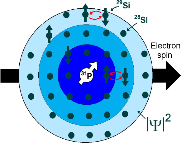
Figure 1: The electron spin of a donor impurity in silicon is sensitive to the magnetic noise produced by nuclear spins within its wave function. When two ²⁹Si isotopes are close to each other, their nuclear spin states may flip-flop due to their mutual dipolar interaction. These flip flop events produce time dependent fluctuations in the electron’s hyperfine field, leading to phase relaxation and spin echo decay.

Recently, we embarked on an effort aimed at understanding the mechanism of electron spin coherence due to nuclear spins from a fully microscopic point of view. In Reference desousa03b we developed a semiclassical model for electron spin echo decay based on the assumption that the relevant nuclear spin dynamics results from pair “flip-flops”, where the spin of two nuclei located close to each other is exchanged due to their mutual dipolar interaction (Fig. 1). The flip-flop processes lead to fluctuations in the nuclear spin hyperfine field seen by the localized electron (e.g., a donor impurity or a quantum dot in a semiconductor). The semiclassical theory is based on the assumption that each flip-flop can be described by a random telegraph noise process (a phenomenological assumption), but with relaxation parameters that can be derived theoretically from a microscopic theory based on the nuclear spin dipolar evolution. Therefore this theory describes the irreversible decay of the effective hyperfine field produced by a pair of nuclear spins on the electron spin. Comparison with experiment chiba72 ; tyryshkin03 ; tyryshkin06 ; abe04 ; ferreti05 suggested reasonable order of magnitude agreement for the 1/e echo decay time (within a factor of 3) but poor qualitative agreement for the time dependence of the echo envelope. The next step was to develop a full quantum theory for the nuclear spin dynamics affecting the electron spin. In reference witzel05 a cluster expansion method was developed to calculate echo decay due to the closed-system dynamics of a group of dipolar coupled nuclear spins, without any stochastic assumption about the nuclear spin dynamics. At lowest order in this cluster expansion the qualitative and quantitative agreement with experimental data was quite good.

In section 4 we develop a fully microscopic theory for the nuclear spin noise spectrum arising due to pair flip-flops induced by the inter-nuclear dipolar interaction. This allows us to give an elegant and simple derivation of the lowest order cluster expansion results of Ref. witzel05 and to interpret these results from the point of view of non-equilibrium statistical mechanics. The full noise spectrum is expressed as a sum of delta-function contributions corresponding to isolated pair flip-flop transitions. We then show that irreversibility can be incorporated into the pair flip-flop processes by adding broadening to these sharp transitions, in a mean-field like approach. Using the method of moments we are able to calculate these broadenings exactly (at infinite temperature). We show explicit numerical results for the noise spectrum affecting a donor impurity in silicon and compare the improved theory with echo decay experiments in natural tyryshkin06 and nuclear-spin-enriched samples abe04 .

2 Noise, relaxation, and decoherence

When the coupling between the spin qubit and the environment is weak, we may write a linearized effective Hamiltonian of the form

$${\cal H}(t)=\frac{1}{2}\gamma B\sigma_{z}+\frac{1}{2}\sum_{q=x,y,z}\hat{\eta}_{q}(t)\sigma_{q},$$ (1)

where $\bm{B}\parallel\hat{z}$ is a static (time independent) magnetic field, $\gamma$ is a gyromagnetic ratio in units of $(sG)^{-1}$ (we set $\hbar=1$ so that energy has units of frequency), $\sigma_{q}$ for $q=x,y,z$ are the Pauli matrices describing qubit observables and $\hat{\eta}_{q}(t)$ represents the environmental (bath) degrees of freedom.

2.1 The Bloch-Wangsness-Redfield master equation

In order to describe the long-time dynamics we may take the limit $t\rightarrow\infty$. Such an approximation is appropriate provided $t\gg\tau_{c}$, where $\tau_{c}$ is a typical correlation time for bath fluctuations (later we will define $\tau_{c}$ properly and relax the long time approximation). In this case spin dynamics can be described by the Bloch-Wangsness-Redfield theory. The average values of the Pauli operator satisfy a Master equation (for a derivation see section 5.11 of Ref. slichter96 )

$$\frac{d}{dt}\langle\bm{\sigma}\rangle=\gamma\bm{B}\times\langle\bm{\sigma}\rangle-\frac{1}{T_{1}}\langle\sigma_{z}\rangle\bm{\hat{z}}-\frac{1}{T_{2x}}\langle\sigma_{x}\rangle\bm{\hat{x}}-\frac{1}{T_{2y}}\langle\sigma_{y}\rangle\bm{\hat{y}},$$ (2)

with

$$\frac{1}{T_{1}} = \frac{\pi}{2}\sum_{q=x,y}\left[\tilde{S}_{q}(+\gamma B)+\tilde{S}_{q}(-\gamma B)\right],$$ (3)

$$\frac{1}{T_{2x}} = \frac{\pi}{2}\left[\tilde{S}_{y}(+\gamma B)+\tilde{S}_{y}(-\gamma B)\right]+\pi\tilde{S}_{z}(0),$$ (4)

$$\frac{1}{T_{2y}} = \frac{\pi}{2}\left[\tilde{S}_{x}(+\gamma B)+\tilde{S}_{x}(-\gamma B)\right]+\pi\tilde{S}_{z}(0).$$ (5)

Here the noise spectrum is defined as

$$\tilde{S}_{q}(\omega)=\frac{1}{2\pi}\int_{-\infty}^{\infty}\textrm{e}^{i\omega t}\langle\hat{\eta}_{q}(t)\hat{\eta}_{q}(0)\rangle dt.$$ (6)

In Eqs. (3), (4), (5) we assume $\langle\hat{\eta}_{q}(t)\hat{\eta}_{q^{\prime}}(0)\rangle=0$ for $q\neq q^{\prime}$. These equations are the generalization of Fermi’s golden rule for coherent evolution. From Eq. (2) we may show that the coherence amplitude $|\langle\sigma_{+}\rangle|=|\langle\sigma_{x}+i\sigma_{y}\rangle|/2$ in a FID experiment decays exponentially with a rate given by

$$\frac{1}{T^{*}_{2}}=\frac{1}{2}\left(\frac{1}{T_{2x}}+\frac{1}{T_{2y}}\right)=\frac{1}{2T_{1}}+\pi\tilde{S}_{z}(0).$$ (7)

In contrast, $T_{1}$ is the time scale for $\langle\sigma_{z}\rangle$ to approach equilibrium, i.e., $T_{1}$ is the energy relaxation time. According to Eq. (7) we have $T^{*}_{2}\leq 2T_{1}$. Note that $T_{1}$ depends on the noise spectrum only at frequencies $+\gamma B$ and $-\gamma B$, a statement of energy conservation. Positive frequency noise can be interpreted as processes where the qubit decays from $\uparrow$ to $\downarrow$ and the environment absorbs an energy quantum $\gamma B$, while negative frequency noise refers to qubit excitation (from $\downarrow$ to $\uparrow$) when the environment emits a quantum $\gamma B$. The correlation time $\tau_{c}$ can be loosely defined as the inverse cut-off for $\tilde{S}_{q}(\omega)$, i.e., for $\omega\gg 1/\tau_{c}$ we may approximate $\tilde{S}_{q}(\omega)\approx 0$.

The Master equation [Eq. (2)] leads to a simple exponential time dependence for all qubit observables. Actually this is not true in many cases of interest, including the case of a phosphorus impurity in silicon where this approximation fails completely (for Si:P the observed free induction decay is approximately $\exp{[-(t/T_{2}^{*})^{2}]}$, while the echo can be fitted to $\exp{[-(2\tau/T_{2})^{2.3}]}$). The problem lies in the fact that the $t\rightarrow\infty$ assumption averages out finite frequency fluctuations; note that $T^{*}_{2}$ differs from $T_{1}$ only via static noise [$\tilde{S}_{z}(0)$ in Eq. (7)]. A large number of pulse spin resonance experiments are sensitive to finite frequencies only [the most notable example is the spin echo, which is able to remove $\tilde{S}_{z}(0)$ completely]. Therefore one must develop a theory for coherent evolution that includes finite frequency fluctuations. Analytical results can be derived if we have $\hat{\eta}_{q}=0$ for $q=x,y$ (the pure dephasing limit) and $\hat{\eta}_{z}$ is distributed according to Gaussian statistics. For many realistic problems the pure dephasing limit turns out to be a good approximation to describe phase relaxation. A common situation is that the neglected components $\tilde{S}_{x,y}(\omega)$ are much smaller than $\tilde{S}_{z}(\omega)$ for positive frequencies much smaller than the qubit energy splitting. For example, in the case of a localized electron spin in a semiconductor, $\tilde{S}_{x,y}(\omega)\propto\omega^{5}$ due to the combination of the spin-orbit and electron phonon interactions desousa03c . As a result, $\tilde{S}_{x,y}(\omega)\ll\tilde{S}_{z}(\omega)$ as $\omega\rightarrow 0$. The Gaussian approximation is described below.

2.2 Finite frequency phase fluctuations and coherence decay in the Gaussian approximation

In many cases of interest, the environmental variable $\hat{\eta_{z}}$ is a sum over several dynamical degrees of freedom, and measurement outcomes for the operator $\hat{\eta}_{z}$ may assume a continuum of values between $-\infty$ and $+\infty$. In those situations we often can resort to the Central limit theorem which states that the statistics for outcomes $\eta^{\prime}$ follows a Gaussian distribution,

$$P[\hat{\eta}_{z}(t)=\eta^{\prime}]=\frac{1}{\sqrt{2\pi\Delta^{2}}}\exp{\left(-\frac{\eta^{\prime 2}}{2\Delta^{2}}\right)},$$ (8)

with a stationary (time independent) variance given by $\Delta^{2}=\langle\hat{\eta}_{z}^{2}(t)\rangle$. Here $\langle A\rangle=\rm{Tr}\{\hat{\rho}_{\rm B}A\}$ is a thermal average taken over all bath degrees of freedom ($\hat{\rho}_{B}\propto\textrm{e}^{-{\cal H}_{B}/k_{B}T}$ is the canonical density matrix for the bath). We also assume $\langle\hat{\eta}_{z}(t)\rangle=0$, since any constant drift in the noise can be incorporated in the effective $B$ field.

Our problem is greatly simplified if we relate the operator $\hat{\eta}_{z}$ to a Gaussian stochastic process $\eta^{\prime}(t)$ in the following way. For each time $t$, $\eta^{\prime}(t)$ corresponds to a classical random variable, that can be interpreted as the outcome of measurements performed by the qubit on the environment. This allows us take averages over the bath states using Eq. (8). Note that the statement “Gaussian” noise refers specifically to the distribution of noise amplitudes, that is not necessarily related to the spectrum of fluctuations (see below).

Our simplified effective Hamiltonian leads to the following evolution operator [recall that we set $\hat{\eta}_{x,y}\equiv 0$ in Eq. (1)]

$${\cal U}_{\eta}(t,0)=\textrm{e}^{-i\int_{0}^{t}dt^{\prime}{\cal H}(t^{\prime})}=\textrm{e}^{-\frac{i}{2}\sigma_{z}\left[Bt+\int_{0}^{t}\eta^{\prime}(t^{\prime})dt^{\prime}\right]}=\textrm{e}^{-\frac{i}{2}\sigma_{z}\left[Bt+X_{\eta}(t)\right]},$$ (9)

where we define

$$X_{\eta}(t)=\int_{0}^{t}\eta^{\prime}(t^{\prime})dt^{\prime}.$$ (10)

Here the subscript $\eta$ emphasizes that this operator is a functional of the trajectory $\eta^{\prime}(t^{\prime})$. The effect of the distribution of trajectories $\eta^{\prime}$ can be described by assuming the qubit evolves according to the density matrix

$$\rho(t)=\sum_{\eta}p_{\eta}{\cal U}_{\eta}(t,0)\rho_{0}{\cal U}^{{\dagger}}_{\eta}(t,0),$$ (11)

where $p_{\eta}$ denotes the appropriate weight probability for each environmental trajectory and $\rho_{0}$ is the $t=0$ density matrix for the qubit. The coherence envelope at time $t$ averaged over all possible noise trajectories is then

$$\langle\langle\sigma_{+}(t)\rangle\rangle = \rm{Tr}\left\{\sigma_{+}\rho(t)\right\}$$ (12)

$$= \sum_{\eta}p_{\eta}\rm{Tr}\left\{{\cal U}^{{\dagger}}_{\eta}(t,0)\sigma_{+}{\cal U}_{\eta}(t,0)\rho_{0}\right\}$$

$$= \textrm{e}^{iBt}\sum_{\eta}p_{\eta}\textrm{e}^{iX_{\eta}(t)}\rm{Tr}\left\{\sigma_{+}\rho_{0}\right\}$$

$$= \langle\textrm{e}^{iX_{\eta}(t)}\rangle\textrm{e}^{iBt}\rm{Tr}\left\{\sigma_{+}\rho_{0}\right\},$$

where we used the identity $\textrm{e}^{i\alpha\sigma_{z}}\sigma_{+}\textrm{e}^{-i\alpha\sigma_{z}}=\textrm{e}^{2i\alpha}\sigma_{+}$. Here the double average $\langle\langle\cdot\rangle\rangle$ denotes a quantum mechanical average over the qubit basis plus an ensemble average over the noise trajectories $\eta^{\prime}(t)$. We can evaluate the coherence amplitude explicitly by noting that the random variable $X(t)=\int_{0}^{t}\eta^{\prime}(t^{\prime})dt^{\prime}$ is also described by a Gaussian distribution, but with a time dependent variance given by $\sigma_{t}=\langle X^{2}(t)\rangle$. Therefore we have

$$\langle\textrm{e}^{iX_{\eta}(t)}\rangle=\int_{-\infty}^{\infty}\frac{1}{\sqrt{2\pi}\sigma_{t}}\textrm{e}^{-\frac{X^{2}}{2\sigma_{t}^{2}}}\textrm{e}^{iX}=\textrm{e}^{-\frac{1}{2}\sigma_{t}^{2}},$$ (13)

with $\sigma_{t}$ given by

$$\sigma_{t}^{2} = \int_{0}^{t}dt_{1}\int_{0}^{t}dt_{2}\langle\eta^{\prime}(t_{1})\eta^{\prime}(t_{2})\rangle$$ (14)

$$= 2\int_{0}^{t}dt_{1}\int_{0}^{t_{1}}dt_{2}\langle\eta^{\prime}(t_{1})\eta^{\prime}(t_{2})\rangle$$

$$= 2\int_{0}^{t}dt^{\prime}\int_{t^{\prime}/2}^{t-t^{\prime}/2}dT\langle\eta^{\prime}(T+t^{\prime}/2)\eta^{\prime}(T-t^{\prime}/2)\rangle$$

$$= 2\int_{0}^{t}(t-t^{\prime})S(t^{\prime})dt^{\prime}.$$

Here we introduced the time dependent correlation function $S(t^{\prime})=\langle\eta^{\prime}(T+t^{\prime}/2)\eta^{\prime}(T-t^{\prime}/2)\rangle=\langle\eta(t^{\prime})\eta(0)\rangle$, that is independent of a time translation $T$ by virtue of the stationarity assumption. Based on the discussion above, it is natural to include quantum noise effects by making the identification

$$S(t)=\langle\eta^{\prime}(t)\eta^{\prime}(0)\rangle\rightarrow\langle\hat{\eta}_{z}(t)\hat{\eta}_{z}(0)\rangle.$$ (15)

It is straightforward to generalize Eqs. (13) and (14) for echo decay. Instead of free evolution (denoted free induction decay in magnetic resonance), consider the Hahn echo given by the sequence $\pi/2-\tau-\pi-\tau-\rm{echo}$. Here the notation “$\pi/2$” denotes a perfect, instantaneous 90^∘ spin rotation around the x-axis (described by the operator $\textrm{e}^{-\frac{i}{4}\pi\sigma_{x}}$). The notation “$-\tau-$” means the spin is allowed to evolve freely for a time interval $\tau$. “$\pi$” denotes a 180^∘ spin rotation around the x-axis, also referred as a “$\pi$-pulse” (this is described by the operator $\textrm{e}^{-\frac{i}{2}\pi\sigma_{x}}=-i\sigma_{x}$). The initial $\pi/2$ pulse prepares the qubit in the state $\rho_{0}=|y+\rangle\langle y+|$, after which it is allowed to evolve freely for time $\tau$, when the $\pi$-pulse is applied. After this pulse the qubit is allowed to evolve for a time interval $\tau$ again, after which the coherence echo is recorded. Hence the evolution operator is given by

$${\cal U}_{\rm{Hahn}}(2\tau)={\cal U}(2\tau,\tau)(-i\sigma_{x}){\cal U}(\tau,0).$$ (16)

The same procedure leading to Eq. (14) is now repeated in order to calculate the magnitude of the Hahn echo envelope at $t=2\tau$. The quantum average is given by

$$\langle\sigma_{+}(2\tau)\rangle = \rm{Tr}\left\{{\cal U}^{{\dagger}}(\tau,0)(i\sigma_{x}){\cal U}^{{\dagger}}(2\tau,\tau)\sigma_{+}{\cal U}(2\tau,\tau)(-i\sigma_{x}){\cal U}(\tau,0)\rho_{0}\right\}$$ (17)

$$= \rm{Tr}\left\{{\cal U}^{{\dagger}}(\tau,0)\sigma_{x}\textrm{e}^{i\int_{\tau}^{2\tau}dt^{\prime}[B+\eta^{\prime}(t^{\prime})]}\sigma_{+}\sigma_{x}{\cal U}(\tau,0)\rho_{0}\right\}$$

$$= \rm{Tr}\left\{\textrm{e}^{i\int_{\tau}^{2\tau}dt^{\prime}[B+\eta^{\prime}(t^{\prime})]}{\cal U}^{{\dagger}}(\tau,0)\sigma_{-}{\cal U}(\tau,0)\rho_{0}\right\}$$

$$= \textrm{e}^{i\int_{\tau}^{2\tau}dt^{\prime}[B+\eta^{\prime}(t^{\prime})]}\textrm{e}^{-i\int_{0}^{\tau}dt^{\prime}[B+\eta^{\prime}(t^{\prime})]}\rm{Tr}\{\sigma_{-}\rho_{0}\}.$$

Therefore the double average can be conveniently written as

$$\langle\langle\sigma_{+}(2\tau)\rangle\rangle=\textrm{e}^{-iB\int_{0}^{2\tau}s(t^{\prime})dt^{\prime}}\left\langle\textrm{e}^{-i\int_{0}^{2\tau}s(t^{\prime})\eta^{\prime}(t^{\prime})dt^{\prime}}\right\rangle\rm{Tr}\left\{\sigma_{-}\rho_{0}\right\},$$ (18)

with the introduction of an auxiliary echo function $s(t)$. For Hahn echo $s(t)=1$ if $0\leq t<\tau$ and $s(t)=-1$ if $t>\tau$. Note that the first term in Eq. (18) is exactly equal to one, because the Hahn echo is able to completely refocus a constant magnetic field. It is convenient to introduce the noise spectrum in Eq. (18) via $S(t)=\int\textrm{e}^{-i\omega t}\tilde{S}(\omega)d\omega$ in order to get the following expression for the coherence envelope

$$\left|\langle\langle\sigma_{+}(t)\rangle\rangle\right|=\exp{\left[-\int_{-\infty}^{\infty}d\omega\;\tilde{S}(\omega){\cal F}(t,\omega)\right]}.$$ (19)

Here we define a filter function that depends on the echo sequence $s(t^{\prime})$,

$${\cal F}(t,\omega)=\int_{0}^{t}dt^{\prime}s(t^{\prime})\int_{0}^{t^{\prime}}dt^{\prime\prime}s(t^{\prime\prime})\cos{\left[\omega(t^{\prime}-t^{\prime\prime})\right]}.$$ (20)

For free induction decay [$s(t)\equiv 1$] we have

$${\cal F}_{\rm{FID}}(t,\omega)=\frac{1}{2}\frac{\sin^{2}{\left(\omega t/2\right)}}{\left(\omega/2\right)^{2}},$$ (21)

while for the Hahn echo

$${\cal F}_{\rm{Hahn}}(2\tau,\omega)=\frac{1}{2}\frac{\sin^{4}{\left(\omega\tau/2\right)}}{\left(\omega/4\right)^{2}}.$$ (22)

Note that ${\cal F}_{\rm{Hahn}}(2\tau,0)=0$. The Hahn echo filters out terms proportional to $\tilde{S}(0)$ in qubit evolution, this is equivalent to the well known removal of inhomogeneous broadening by the echo. Any spin resonance sequence containing instantaneous $\pi/2$ or $\pi$-pulses (not necessarily equally spaced) can be mapped into an appropriate echo function $s(t)$. An important example is the class of Carr-Purcell sequences that can be used to enhance coherence.

General results for the short time behavior

We may derive interesting results when the time-dependent correlation function $S(t)$ is analytic at $t=0$. In this case we may expand around $t=0$ to obtain

$$S(t) = \langle\eta^{\prime}(t)\eta^{\prime}(0)\rangle=\int_{-\infty}^{\infty}d\omega\textrm{e}^{-i\omega t}\tilde{S}(\omega)$$ (23)

$$= \sum_{n=0}^{\infty}\frac{(-1)^{n}}{(2n)!}M_{2n}t^{2n},$$

with the 2n-th moment of the noise spectrum defined as

$$M_{2n}=\int_{-\infty}^{\infty}d\omega\tilde{S}(\omega)w^{2n}.$$ (24)

Hence if $S(t)$ is analytic at $t=0$, we must have $M_{2n}<\infty$ for all $n$, i.e. the noise spectrum has a well defined high frequency cut-off. It is important to keep in mind that the assumption of analyticity at $t=0$ is actually quite restrictive. Physically, only $M_{0}<\infty$ is required, so that $S(0)<\infty$ (this is the noise power or mean square deviation for $\eta^{\prime}$). Important examples where $S(t)$ is not analytic at $t=0$ include the Gauss-Markov model described below [See Eq. (27)].

If the $t=0$ expansion exists we may immediately obtain the short time behaviors for the free induction decay and Hahn echo:

$$\langle\langle\sigma_{+}(t)\rangle\rangle_{\rm{FID}}=\textrm{e}^{-\int d\omega\tilde{S}(\omega)\frac{1}{2}\frac{\sin^{2}{(\omega t/2)}}{(\omega/2)^{2}}}\approx\textrm{e}^{-\frac{1}{2}M_{0}t^{2}+\frac{1}{24}M_{2}t^{4}},$$ (25)

$$\langle\langle\sigma_{+}(2\tau)\rangle\rangle_{\rm{Hahn}}=\textrm{e}^{-\int d\omega\tilde{S}(\omega)\frac{1}{2}\frac{\sin^{4}{(\omega\tau/2)}}{(\omega/4)^{2}}}\approx\textrm{e}^{-\frac{1}{2}M_{2}\tau^{4}+\frac{1}{12}M_{4}\tau^{6}}.$$ (26)

The short time behavior described by Eqs. (25), (26) is universal for noise spectra possessing a high frequency cut-off. Note the striking difference in time dependence: For free induction decay the coherence behaves as $\sim\textrm{e}^{-t^{2}}$, while for a Hahn echo we have $\sim\textrm{e}^{-\tau^{4}}$. This happens because the Hahn echo is independent of the mean square deviation $M_{0}=S(0)$.

Example: The Gauss-Markov model

The simplest model of Brownian motion assumes a phenomenological correlation function that decays exponentially in time,

$$S(t)=\Delta^{2}\exp{\left(-|t|/\tau_{c}\right)},$$ (27)

where $\tau_{c}$ is a correlation time that describes the “memory” of the environmental noise. This model is useful e.g. in liquid state NMR in order to calculate the line-widths of a molecule diffusing across an inhomogeneous magnetic field. In that case, $\Delta$ becomes the typical field inhomogeneity, while the “speed” for diffusion is of the order of $\Delta/\tau_{c}$. The resulting environmental noise spectrum [Fourier transform of Eq. (27)] is a Lorentzian, given by

$$\tilde{S}(\omega)=\frac{\Delta^{2}\tau_{c}}{\pi}\frac{1}{\left(\omega\tau_{c}\right)^{2}+1}.$$ (28)

We start by discussing free induction decay. Using Eqs. (18) and (27) with $s(t^{\prime})=1$, we get

$$\left|\langle\langle\sigma_{+}(t)\rangle\rangle\right|_{{\rm FID}}=\exp{\left\{-\Delta^{2}\tau_{c}^{2}\left[t/\tau_{c}+\left(\textrm{e}^{-t/\tau_{c}}-1\right)\right]\right\}}.$$ (29)

For $t\gg\tau_{c}$, Eq. (29) leads to

$$|\langle\langle\sigma_{+}(t)\rangle\rangle|_{{\rm FID}}\approx\textrm{e}^{-\Delta^{2}\tau_{c}t}.$$ (30)

In this regime, the correlation function Eq. (27) can be approximated by a delta function, and the decay is a simple exponential signaling that a Master equation approach is appropriate [Eq. (2)]. The coherence time is given by $T^{*}_{2}=1/(\Delta^{2}\tau_{c})$. Interestingly, as $\tau_{c}\rightarrow 0$ with $\Delta$ finite, $T^{*}_{2}\rightarrow\infty$. This phenomenon is known as motional narrowing, inspired by the motion of molecules in a field gradient. The faster the molecule is diffusing, the narrower is its resonance line. Now we look at the low frequency noise limit, $t\ll\tau_{c}$. This leads to

$$|\langle\langle\sigma_{+}(t)\rangle\rangle|_{{\rm FID}}\approx\textrm{e}^{-\frac{1}{2}\Delta^{2}t^{2}}\equiv\textrm{e}^{-\left(t/T_{2}^{*}\right)^{2}}.$$ (31)

In contrast to Eq. (30), the decay differs from a simple exponential and is independent of $\tau_{c}$. This result is equivalent to an average over an ensemble of qubits at any specific time $t$ (in other words, the line-width $\Delta/\sqrt{2}$ and dephasing time $T_{2}^{*}=\sqrt{2}/\Delta$ are a consequence of inhomogeneous broadening). Therefore the coherence decay is completely independent of the environmental kinetics. As we shall see below, this decay is to a large extent reversible by the Hahn echo.

The Hahn echo decay is calculated from Eqs. (19), (22), and (28) leading to

$$\langle\langle\sigma_{+}(2\tau)\rangle\rangle_{{\rm Hahn}}=\exp{\left\{-\Delta^{2}\tau_{c}^{2}\left[2\tau/\tau_{c}-3+4\textrm{e}^{-\tau/\tau_{c}}-\textrm{e}^{-2\tau/\tau_{c}}\right]\right\}}.$$ (32)

For $\tau\gg\tau_{c}$ we again have motional narrowing, $\langle\langle\sigma_{+}(2\tau)\rangle\rangle_{{\rm Hahn}}\approx\textrm{e}^{-\Delta^{2}\tau_{c}2\tau}$, a result identical to FID [Eq. (30)] if we set $t=2\tau$. This occurs because the noise trajectories are completely uncorrelated before and after the $\pi$-pulse, that plays no role in this limit. For $\tau\ll\tau_{c}$ we get

$$\langle\langle\sigma_{+}(2\tau)\rangle\rangle_{{\rm Hahn}}\approx\textrm{e}^{-\frac{1}{24}\left(\Delta\tau_{c}\right)^{2}\left(\frac{2\tau}{\tau_{c}}\right)^{3}}\approx\textrm{e}^{-\left(\frac{2\tau}{T_{2}}\right)^{3}}.$$ (33)

In drastic contrast to free induction decay, Eq. (33) depends crucially on the kinetic variable $\tau_{c}$. The time scale $T_{2}$ for 1/e decay of Hahn echo is considerably longer than $T_{2}^{*}$ when $\Delta\gg\tau_{c}$.

A train of Hahn echoes: The Carr-Purcell sequence and coherence control

Consider the sequence $\pi/2-\left[\tau-\pi-\tau-\rm{echo}\right]_{\rm{repeat}}$. It consists of the application of a $\pi$-pulse every odd multiple of $\tau$, with the observation of an echo at even multiples of $\tau$, i.e. at $t=2n\tau$ for $n$ integer. In the limit $\tau\ll\tau_{c}$ the $n$-th echo envelope can be approximated by a product of $n$ Hahn echoes,

$$\langle\langle\sigma_{+}(2n\tau)\rangle\rangle_{\rm{CP}}\approx\langle\langle\sigma_{+}(2\tau)\rangle\rangle^{n}_{\rm{Hahn}}\approx\textrm{e}^{-\frac{2n\tau}{T_{2}}\left(\frac{2\tau}{T_{2}}\right)^{2}}\equiv\textrm{e}^{-\frac{2n\tau}{T_{2}^{\rm{eff}}}},$$ (34)

with $T_{2}^{\rm{eff}}\equiv T_{2}\left[T_{2}/(2\tau)\right]^{2}$. As $\tau$ is decreased below $T_{2}$ the effective coherence time $T_{2}^{\rm{eff}}$ increases proportional to $1/\tau^{2}$. Therefore a train of Hahn echoes can be used to control decoherence. Rewriting Eq. (34) with $t\equiv 2n\tau$ we get $T_{2}^{\rm{eff}}=(2n)^{2/3}T_{2}$, showing that the scaling of the enhanced coherence time with the number of $\pi$-pulses is sub-linear. The train of $\pi$-pulses spaced by $\tau\ll\tau_{c}$ effectively averages out the noise, because within $\tau$ much shorter than $\tau_{c}$ the noise appears to be time-independent.

Loss of visibility due to high frequency noise

In order to understand the role of high frequency noise, consider the model Lorentzian noise spectrum peaked at frequency $\Omega$ with a broadening given by $1/\tau_{d}$,

$$\tilde{S}_{L}(\omega)=\frac{\Delta^{2}\tau_{d}}{\pi}\frac{1}{\left(\omega-\Omega\right)^{2}\tau_{d}^{2}+1}.$$ (35)

Using Eqs. (19) and (21) and assuming $\Omega\gg 1/\tau_{d}$ we get

$$\left|\langle\langle\sigma_{+}(t)\rangle\rangle\right|_{L}\approx\exp{\left[-2\left(\frac{\Delta}{\Omega}\right)^{2}\left(1-\textrm{e}^{-t/\tau_{d}}\cos{\Omega t}\right)\right]}.$$ (36)

Therefore high frequency noise leads to loss of visibility for the coherence oscillations. The loss of visibility is initially oscillatory, but decays exponentially to a fixed contrast for $t\gg\tau_{d}$. For comparison consider the Gaussian model,

$$\tilde{S}_{G}(\omega)=\frac{\Delta^{2}}{\sqrt{2\pi\sigma^{2}}}\exp{\left[-\frac{(\omega-\Omega)^{2}}{2\sigma^{2}}\right]}.$$ (37)

For $\Omega\gg\sigma$ we get

$$\left|\langle\langle\sigma_{+}(t)\rangle\rangle\right|_{G}\approx\exp{\left[-2\left(\frac{\Delta}{\Omega}\right)^{2}\left(1-\textrm{e}^{-\frac{1}{2}\sigma^{2}t^{2}}\cos{\Omega t}\right)\right]}.$$ (38)

Note that the difference between the Gaussian and the Lorentzian models lies in the time dependence of the approach to a fixed contrast. Deviations from Lorentzian behavior may be assigned to non-exponential decays of the coherence envelope. Although Eqs. (36), (38) were calculated for free induction decay, it is also a good approximation for Hahn echoes in the limit $\Omega\gg 1/\tau$.

2.3 Single spin measurement versus ensemble experiments: Different coherence times?

Recently single shot detection of the spin of a single electron in a GaAs quantum dot was demonstrated elzerman04 , and the Hahn echo decay of the singlet-triplet transition in a double quantum dot was measured petta05 . Also, spin resonance of a single spin center in the Si/SiO₂ interface was detected through time averaged current fluctuations xiao04 . These state of the art experiments should be contrasted with the traditional spin resonance measurements where the microwave excitation of a sample containing a large number of localized spins is probed. Naturally the following question arises: Are the coherence times extracted from an ensemble measurement any different from the ones obtained in single spin experiments?

The answer to this question is related to the ergodicity of the environment producing noise, i.e., whether time averages are equal to ensemble averages. Even when single shot read-out of a quantum degree of freedom is possible, one must repeat each measurement several times, in order to obtain good average values for the observables. For example, measurements of the state of a single spin yields two possible outcomes and one must time-average an ensemble of identical qubit evolutions in order to obtain an average value that reflects the correct outcome probabilities (In Ref. elzerman04 , each average value resulted from $\sim 600$ read-out traces). The presence of phase fluctuation with correlation time $\tau_{c}$ smaller than the typical averaging time implies spin precession with distinct frequencies for read-out traces separated in time. This may lead to strong free induction decay (low $T_{2}^{*}$) in a single shot read-out measurement, see Fig. 2. This was indeed observed in the double-dot experiments of Petta et al petta05 .

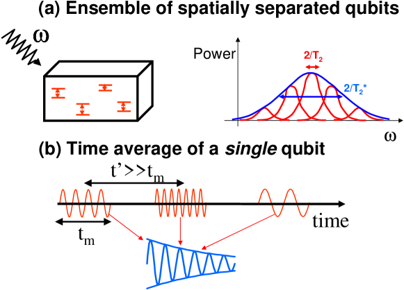
Figure 2: (a) A Traditional spin resonance experiment probes the coherent evolution of an ensemble of spatially separated spins. The spins can be separated into different “packets” with similar resonance frequencies, each packet with linewidth $2/T_{2}$. A free induction decay measurement is sensitive to the broadened linewidth $2/T_{2}^{*}$. A spin echo is needed in order to reveal the intrinsic linewidth $2/T_{2}$. (b) A similar situation applies to single spin experiments subject to low frequency noise, because each time ensemble may have a different resonance frequency

The free induction decay time $T_{2}^{*}$ in ensemble experiments may be quite different from single-spin experiments. This is because the spatial separation of spins adds several new contributions to zero frequency noise. These include spatially inhomogeneous magnetic fields, $g$-factors, and strains. However, all these contributions are removed by a Hahn echo sequence, that filters out environmental fluctuations with frequencies smaller than $1/\tau$. Therefore we expect the spin echo decay time $T_{2}$ for a spatial ensemble and a single spin to be similar, provided the mechanisms for finite frequency noise do not vary wildly for spatially separated spins, and the environment affecting each individual spin is ergodic within the average time scale (similar reasoning applies for $T_{1}$, which is determined by high frequency noise $\omega=\gamma B$).

The Gaussian theory of decoherence described here is appropriate for ergodic environments. It would be very interesting to explore model systems both experimentally and theoretically in order to search for detectable non-ergodic effects in coherent evolution.

3 Electron spin evolution due to nuclear spins: Isotropic and anisotropic hyperfine interactions, inter-nuclear couplings and the secular approximation

A localized electron spin coupled to a lattice of interacting nuclear spins provides a suitable model system for the microscopic description of environmental fluctuations affecting coherent evolution. Here we describe a model appropriate for localized electron spins in semiconductors, and discuss some approximations that can be made in a moderate magnetic field (typically larger than the inhomogeneous broadening linewidth, $B>0.1$ T).

3.1 The electron-nuclear spin Hamiltonian

The full Hamiltonian for a single electron interacting with N nuclear spins is given by slichter96

$${\cal H}={\cal H}_{eZ}+{\cal H}_{nZ}+{\cal H}_{en}+{\cal H^{\prime}}_{en}+{\cal H}_{nn}.$$ (39)

Here the Zeeman energies for electron and nuclear spins are respectively

$${\cal H}_{eZ} = \frac{1}{2}\gamma_{e}B\sigma_{z}$$ (40)

$${\cal H}_{nZ} = -\gamma_{n}B\sum_{i}I_{iz},$$ (41)

where $\bm{\sigma}=(\sigma_{x},\sigma_{y},\sigma_{z})$ is the Pauli matrix vector representing the electron spin, and $\bm{I}_{i}$ is the nuclear spin operator for a nucleus located at position $\bm{R}_{i}$ with respect to the center of the electron wave function. For $B=1$ T we have $\gamma_{e}B\sim 10^{11}$ Hz while $\gamma_{n}B\sim 10^{8}$ Hz. The $e-n$ coupling takes place due to isotropic and anisotropic hyperfine interactions. The isotropic hyperfine interaction is given by

$${\cal H}_{en}=\frac{1}{2}\sum_{i}A^{\rm{iso}}_{i}\bm{I}_{i}\cdot\bm{\sigma},$$ (42)

with contact hyperfine interaction

$$A^{\rm{iso}}_{i}=\frac{8\pi}{3}\gamma_{e0}\gamma_{n}\hbar\left|\Psi(\bm{R}_{i})\right|^{2},$$ (43)

where $\gamma_{e0}=e/(m_{e}c)=1.76\times 10^{7}$ (sG)^-1 is the gyromagnetic ratio for a free electron and $\Psi(\bm{r})$ is the electron’s wave function. Typical values of $A^{\rm{iso}}_{i}$ varies from $A^{\rm{iso}}_{i}\sim 10^{7}$ Hz for $\bm{R}_{i}=0$ (at the center of a donor impurity wave function) to $A^{\rm{iso}}_{i}\sim 0$ for $R_{i}$ much larger than the impurity Bohr radius. The anisotropic hyperfine interaction reads

$${\cal H^{\prime}}_{en}=\frac{1}{2}\sum_{i}\bm{I}_{i}\cdot\bm{A^{\prime}}_{i}\cdot\bm{\sigma}$$ (44)

with an anisotropic hyperfine tensor given by

$$(\bm{A}^{\prime}_{i})_{lm}=\gamma_{e0}\gamma_{n}\hbar\int d^{3}r|\Psi(\bm{r}-\bm{R}_{i})|^{2}\left(\frac{2r}{2r+r_{0}}\right)\left(\frac{3x_{l}x_{m}}{r^{5}}-\frac{\delta_{lm}}{r^{3}}\right),$$ (45)

where $r_{0}=e^{2}/(m_{e}c^{2})$ is the classical electron radius. Note that Eqs. (42) and (44) are first order perturbative corrections in the electron coordinate $\bm{r}$. Finally, the nuclear-nuclear dipolar coupling reads

$${\cal H}_{nn}=\gamma_{n}^{2}\hbar\sum_{i<j}\left[\frac{\bm{I}_{i}\cdot\bm{I}_{j}}{R_{ij}^{3}}-\frac{3\left(\bm{I}_{i}\cdot\bm{R}_{ij}\right)\left(\bm{I}_{j}\cdot\bm{R}_{ij}\right)}{R_{ij}^{5}}\right],$$ (46)

where $\bm{R}_{ij}=\bm{R}_{i}-\bm{R}_{j}$ is the distance between two nuclei. The typical energy scale for Eq. (46) is a few KHz for nearest-neighbors in a crystal.

The full Hamiltonian Eq. (39) is a formidable many-body problem. It is particularly hard to study because of the lack of symmetry. In order to study theoretically the quantum dynamics of an electron subject to a large number of nuclear spins we need to truncate Eq. (39). Here we discuss some simplifications appropriate for $B>0.1$ T, a condition typically satisfied in several experiments. The first approximation arises when we note that the electron Zeeman energy is typically $~{}10^{3}$ times larger than the nuclear Zeeman energy. For $B>100$ G the former is much larger than $A^{\rm{iso}}_{i}$, therefore the electron spin cannot be “flipped” by the action of the hyperfine interaction. In other words, “real” $e-n$ flip-flop transitions get inhibited at these fields (however virtual transitions induced by second order processes such as ${\cal H}_{en}^{2}$ do produce visible effects as discussed in section 3.3). This consideration allows us to approximate the isotropic hyperfine interaction to a diagonal form (secular approximation),

$${\cal H}_{en}\approx\frac{1}{2}\sigma_{z}\sum_{i}A^{\rm{iso}}_{i}I_{iz}.$$ (47)

The anisotropic hyperfine interaction contains a similar diagonal contribution in addition to pseudo-secular terms of the form $\sigma_{z}I_{i\pm}$. These terms lead to important echo modulations of the order of $\sim(A^{\prime}_{i}/\gamma_{n}B)^{2}\sim 0.1-1$ for moderate magnetic fields ($B\sim 0.1-1$ T). To derive these terms, assume $\hat{b}$ as the direction of the magnetic field and substitute $\bm{\sigma}\rightarrow\sigma_{z}\hat{b}$ in Eq. (44). The result is

$${\cal H^{\prime}}_{en}\approx\frac{1}{2}\sigma_{z}\sum_{i}\left(A^{\prime}_{i\parallel}I_{iz}+A^{\prime}_{i\perp}I_{i+}+A^{\prime*}_{i\perp}I_{i-}\right),$$ (48)

where

$$A^{\prime}_{i\parallel} = \hat{z}\cdot\bm{A^{\prime}}_{i}\cdot\hat{b},$$ (49)

$$A^{\prime}_{i\perp} = \frac{1}{2}\left[\hat{x}\cdot\bm{A^{\prime}}_{i}\cdot\hat{b}+i\hat{y}\cdot\bm{A^{\prime}}_{i}\cdot\hat{b}\right].$$ (50)

For some lattice sites (closer to the center of the donor impurity) $A^{\prime}_{i\perp}$ is a reasonable fraction of the nuclear spin Zeeman energy (even for $B\sim 1$ Tesla), and as a consequence the precession axis of these nuclear spins will depend on the state of the electron, producing strong modulations in the nuclear spin echo signal saikin03 . For the electron spin Eq. (48) produces small modulations observed at the shortest time scales in the echo decay envelope abe04 . Finally, we can neglect contributions to Eq. (46) that do not conserve nuclear spin Zeeman energy,

$${\cal H}_{nn}\approx\sum_{i<j}b_{ij}\left(I_{i+}I_{j-}+I_{i-}I_{j+}-4I_{iz}I_{jz}\right),$$ (51)

with

$$b_{ij}=-\frac{1}{4}\gamma_{n}^{2}\hbar\frac{1-3\cos^{2}{\theta_{ij}}}{R_{ij}^{3}}.$$ (52)

Here $\theta_{ij}$ is the angle formed by the applied $\bm{B}$ field and the vector $\bm{R_{ij}}$ linking the two nuclear spins $i,j$. This leads to an important orientation dependence of coherence times.

3.2 Electron-nuclear spin evolution in the secular approximation

In the secular approximation [Eqs. (47)-(51)] the electron-nuclear spin Hamiltonian is block-diagonal,

$${\cal H}={\cal H}_{+}\mid\Uparrow\rangle\langle\Uparrow\mid+{\cal H}_{-}\mid\Downarrow\rangle\langle\Downarrow\mid,$$ (53)

where $\mid\Uparrow\rangle\langle\Uparrow\mid$ and $\mid\Downarrow\rangle\langle\Downarrow\mid$ are projectors in the electron spin up and down subspaces respectively. Here ${\cal H}_{\pm}$ contains only nuclear spin operators and is given by

$${\cal H}_{\pm} = {\cal H}_{nn}-\gamma_{n}B\sum_{i}I_{iz}\pm\frac{1}{2}\gamma_{e}B$$ (54)

$$\pm\frac{1}{2}\sum_{i}\left[A_{i}I_{iz}+A^{\prime}_{i}I_{i+}+A^{\prime*}_{i}I_{i-}\right],$$

where $A_{i}\equiv A^{\rm{iso}}_{i}+A^{\prime}_{i\parallel}$ and $A^{\prime}_{i}\equiv A^{\prime}_{i\perp}$. Accordingly, the evolution operator becomes ${\cal U}(t)={\cal U}_{+}(t)\mid\Uparrow\rangle\langle\Uparrow\mid+{\cal U}_{-}(t)\mid\Downarrow\rangle\langle\Downarrow\mid$, with ${\cal U}_{\pm}(t)=\textrm{e}^{-it{\cal H}_{\pm}}$. We can write an explicit expression for the coherences as a function of the evolution operators ${\cal U}_{\pm}(t)$ provided the initial density matrix can be written in product form, $\rho_{0}=\rho_{0e}\otimes\rho_{0n}$. The free induction decay is given by

$$\langle\sigma_{+}(t)\rangle_{\rm{FID}} = \rm{Tr}_{n}\rm{Tr}_{e}\left\{{\cal U}^{{\dagger}}\sigma_{+}{\cal U}\rho_{0e}\otimes\rho_{0n}\right\}$$ (55)

$$= \rm{Tr}_{n}\left\{{\cal U}^{{\dagger}}_{+}{\cal U}_{-}\rho_{0n}\right\}\rm{Tr}_{e}\left\{\sigma_{+}\rho_{0e}\right\},$$

where we used the fact that ${\cal U}^{{\dagger}}\sigma_{+}{\cal U}={\cal U}^{{\dagger}}_{+}{\cal U}_{-}\mid\Uparrow\rangle\langle\Downarrow\mid$, and $\sigma_{+}=\mid\Uparrow\rangle\langle\Downarrow\mid$. For the Hahn echo, we use ${\cal U}(\tau)\sigma_{x}{\cal U}(\tau)$ as our evolution operator, to get

$$\langle\sigma_{+}(2\tau)\rangle_{\rm{Hahn}}=\rm{Tr}_{n}\left\{{\cal U}^{{\dagger}}_{-}{\cal U}^{{\dagger}}_{+}{\cal U}_{-}{\cal U}_{+}\rho_{0n}\right\}\rm{Tr}_{e}\left\{\sigma_{-}\rho_{0e}\right\}.$$ (56)

Eqs. (55) and (56) are exact in the secular approximation, and make explicit the dependence of the electron’s coherence envelope in the nuclear spin Hamiltonian evolution.

Inhomogeneous broadening due to the isotropic hyperfine interaction

The diagonal model

$${\cal H}_{\pm}=-\gamma_{n}B\sum_{i}I_{iz}\pm\frac{1}{2}\gamma_{e}B\pm\frac{1}{2}\sum_{i}A_{i}I_{iz}$$ (57)

is easily solved exactly for nuclear spins initially in a product state. Assume the electron spin is pointing in the $+y$ direction, and the nuclear spin states are distributed randomly, each nuclei with equal probability of pointing up or down. The free induction decay amplitude becomes

$$\langle\sigma_{+}(t)\rangle_{\rm{FID}} = \frac{i}{2}\rm{Tr}_{n}\left\{{\cal U}^{{\dagger}}_{+}{\cal U}_{-}\right\}$$ (58)

$$= \frac{i}{2}\textrm{e}^{i\gamma_{e}Bt}\prod_{j}\frac{1}{2}\left[\textrm{e}^{\frac{i}{2}A_{j}t}+\textrm{e}^{-i\frac{i}{2}A_{j}t}\right]$$

$$= \frac{i}{2}\textrm{e}^{i\gamma_{e}Bt}\sum_{\xi_{1}=\pm 1,\ldots}\frac{1}{2^{N}}\textrm{e}^{\frac{i}{2}t\sum_{j}A_{j}\xi_{j}}$$

$$\approx \frac{i}{2}\textrm{e}^{i\gamma_{e}Bt}\textrm{e}^{-\frac{1}{8}t^{2}\sum_{j}A_{j}^{2}},$$

where in the last line we assumed $N\rightarrow\infty$ with each individual $A_{i}\rightarrow 0$ so that the hyperfine field can be approximated by a continuous Gaussian distribution. The free induction decay rate or inhomogeneously broadened linewidth is given by $\frac{1}{T_{2}^{*}}\sim A_{\rm{rms}}=\sqrt{\sum_{j}A_{j}^{2}}$. This fast decay rate should be compared to the Hahn echo: From Eq. (56) we see that $\langle\sigma_{+}(2\tau)\rangle_{\rm{Hahn}}=-i/2$, the Hahn echo never decays. In fact, from Eq. (56) we can easily prove that the class of Hamiltonians of the form Eq. (53) satisfying $\left[{\cal H}_{+},{\cal H}_{-}\right]=0$ have time independent Hahn echoes given by $\rm{Tr}\{\sigma_{-}\rho_{0e}\}$ shenvi05b .

3.3 Beyond the secular approximation: Nuclear-nuclear interactions mediated by the electron spin hyperfine interaction

In the sections above we showed that the secular approximation allows us to decouple electron spin dynamics from nuclear spin dynamics completely. This approximation clearly does not hold at low magnetic fields, and the problem becomes considerably more complicated. The study of electron spin evolution subject to the full isotropic hyperfine interaction has attracted a great deal of attention lately merkulov02 ; khaetskii02 ; shenvi05b ; deng06 , particularly because of a series of free induction decay experiments probing electron spin dynamics in quantum dots in the low magnetic field regime gammon01 . In the author’s opinion the most successful theoretical approach so far in the description of these experiments is to treat the collective nuclear spin field classically by taking averages over its direction and magnitude merkulov02 . Here we shall not discuss the interesting effects occurring at low fields. Instead, we will focus on the following question: What is the threshold field $B_{\rm th}$ for the secular approximation to hold? For intermediate $B>B_{\rm th}$ (not satisfying $B\gg B_{\rm th}$), how can the non-secular terms be incorporated in a block diagonal Hamiltonian of the form Eq. (53)?

In order to answer these questions, let’s consider the Hamiltonian

$${\cal H}={\cal H}_{0}+{\cal V},$$ (59)

$${\cal H}_{0}=\frac{1}{2}(\gamma_{e}+\gamma_{n})B\sigma_{z}+\frac{1}{2}\sigma_{z}\sum_{j}A_{j}I_{jz},$$ (60)

$${\cal V}=\frac{1}{2}\sum_{j}A_{j}\left(\sigma_{+}I_{j-}+\sigma_{-}I_{j+}\right),$$ (61)

where ${\cal H}_{0}$ and ${\cal V}$ denote the secular and non-secular contributions respectively. Here we remove the nuclear Zeeman energy by transforming to the rotating frame precessing at $\gamma_{n}B$. From Eq. (61) we may be tempted to assume that flip-flop processes involving an electron and a nuclear spin (e.g., $\Uparrow\downarrow\rightarrow\Downarrow\uparrow$) are forbidden by energy conservation at fields $\gamma_{e}B\gg A_{i}$. However, the situation is much more complex because higher order “virtual” processes such as ${\cal V}^{2}=A_{i}A_{j}I_{i+}I_{j-}\sigma_{+}\sigma_{-}+\cdots$ preserve the electron spin polarization and hence may have a small energy cost (of the order of $A_{i}-A_{j}$ for $A_{i}\sim A_{j}$). As we show below, these processes actually lead to a long-range effective coupling between nuclear spins, similar to the RKKY interaction between nuclear spins in a metal. We will show this using the original self-consistent approach of Shenvi et al.

Let $\left|\psi^{+}\right\rangle$ be a “+” eigenstate of the Hamiltonian Eq. (59), i.e. $\left|\psi^{+}\right\rangle$ has primarily electron spin-up character. Without loss of generality, $\left|\psi^{+}\right\rangle$ can be written as

$$\left|\psi^{+}\right\rangle=\left|\Uparrow,\psi_{\Uparrow}^{+}\right\rangle+\left|\Downarrow,\psi_{\Downarrow}^{+}\right\rangle.$$ (62)

Because the perturbation ${\cal V}$ flips the polarization of the electron, the action of ${\cal H}$ on the electron spin-up and electron spin-down subspaces yields the two simultaneous equations,

$${\cal H}_{0}\left|\Uparrow,\psi_{\Uparrow}^{+}\right\rangle+{\cal V}\left|\Downarrow,\psi_{\Downarrow}^{+}\right\rangle = E_{+}\left|\Uparrow,\psi_{\Uparrow}^{+}\right\rangle,$$ (63)

$${\cal H}_{0}\left|\Downarrow,\psi_{\Downarrow}^{+}\right\rangle+{\cal V}\left|\Uparrow,\psi_{\Uparrow}^{+}\right\rangle = E_{+}\left|\Downarrow,\psi_{\Downarrow}^{+}\right\rangle.$$ (64)

Eq. (64) can be solved for $\left|\Downarrow,\psi_{\Downarrow}^{+}\right\rangle$ and the resulting expression inserted into Eq. (63) yields

$${\cal H}_{0}\left|\Uparrow,\psi_{\Uparrow}^{+}\right\rangle+{\cal V}\frac{1}{E_{+}-{\cal H}_{0}}{\cal V}\left|\Uparrow,\psi_{\Uparrow}^{+}\right\rangle=E_{+}\left|\Uparrow,\psi_{\Uparrow}^{+}\right\rangle.$$ (65)

In the presence of an energy gap between the spin-up and spin-down states (this is certainly true at high magnetic fields satisfying $B>\sum A_{j}/\gamma_{e}$), the operator $1/(E_{+}-{\cal H}_{0})$ is always well-defined shenvi05a . Because the left-hand side of Eq. (65) depends on $E_{+}$, it is not a true Schrödinger equation; to obtain $E_{+}$ exactly, Eq. (65) must be solved self-consistently. However, if we use $E_{+}\approx(\gamma_{e}+\gamma_{n})B/2$, then we can obtain an effective Hamiltonian from Eq. (65). The effective Hamiltonian in the electron spin-up subspace is

$${\cal H}_{\mathrm{eff}}^{+} = {\cal H}_{0}+{\cal V}_{\mathrm{eff}}^{+}$$ (66)

$${\cal V}_{\mathrm{eff}}^{+} = \frac{1}{4}\sum_{j,k}{A_{j}A_{k}I_{j-}\frac{1}{(\gamma_{e}+\gamma_{n})B+\frac{1}{2}\sum_{j}{A_{j}I_{jz}}}I_{k+}}.$$ (67)

We obtain a similar, but not identical, effective Hamiltonian for the spin-down subspace (note the transposition of the $I_{-}$ and $I_{+}$ operators),

$${\cal H}_{\mathrm{eff}}^{-} = {\cal H}_{0}+{\cal V}_{\mathrm{eff}}^{-}$$ (68)

$${\cal V}_{\mathrm{eff}}^{-} = -\frac{1}{4}\sum_{j,k}{A_{j}A_{k}I_{j+}\frac{1}{(\gamma_{e}-\gamma_{n})B+\frac{1}{2}\sum_{j}{A_{j}I_{jz}}}I_{k-}}.$$ (69)

Eqs. (67) and (69) show that the overall coupling between nuclei does indeed decrease at high fields, because the operator $1/(E-{\cal H}_{0})$ scales approximately as $1/B$. However, the energy cost for flip-flopping two nuclei $j$ and $k$ is proportional to $A_{j}-A_{k}$. Thus, if $A_{j}$ and $A_{k}$ are close in value, the nuclei can flip-flop even at high fields. Eqs. (67), (69) were later derived using an alternative canonical transformation approach yao05 .

We may expand Eqs. (67) and (69) in powers of $\sum_{j}A_{j}I_{jz}/(\gamma_{e}B)$, so that for the unpolarized case we have approximately

$${\cal V}_{\rm{eff}}\approx\frac{1}{2}\sigma_{z}\sum_{j,k}\frac{A_{j}A_{k}}{2(\gamma_{e}+\gamma_{n})B}I_{j+}I_{k-}.$$ (70)

This effective Hamiltonian is of the secular type Eq. (53), and satisfies the symmetry condition $\left[{\cal H}_{+},{\cal H}_{-}\right]=0$. Therefore a Hahn echo is able to refocus this interaction completely.

Shenvi et al performed exact numerical calculations of electron spin echo dynamics in clusters of $N=13$ nuclear spins shenvi05b . The Hahn echo envelope was found to decay fast to a loss of contrast given by

$$\left|\langle\sigma_{+}(2\tau)\rangle\right|\approx\frac{1}{2}-\frac{\sum_{j}A_{j}^{2}}{\left[(\gamma_{e}+\gamma_{n})B\right]^{2}}.$$ (71)

This shows that the threshold field for neglecting the non-secular isotropic hyperfine interaction in the Hahn echo is given by the inhomogeneously broadened linewidth, $B_{\rm th}=\sqrt{\sum_{j}A_{j}^{2}}/\gamma_{e}\sim 10-100$ G (for a donor impurity in silicon, $B_{\rm th}$ is $\approx 1$ G for natural samples and $\approx 10$ G for ²⁹Si enriched samples).

Recently, Yao et al yao05 and Deng et al. deng06 showed that the electron-mediated inter-nuclear coupling may be observed as a magnetic field dependence of the free induction decay time in small quantum dots. There is currently an interesting debate on the correct form of the time dependence for FID decay. Yao et al. derived the FID decay from Eq. (70) and obtained $\langle\sigma_{+}(t)\rangle\sim\textrm{e}^{-t^{2}}$, while Deng et al. carried out a full many-body calculation to argue that FID scales as a power law according to $\langle\sigma_{+}(t)\rangle\sim 1/t^{2}$.

4 Microscopic calculation of the nuclear spin noise spectrum and electron spin decoherence

In this section we discuss low frequency noise due to interacting nuclear spins. For simplicity, we assume only isotropic hyperfine interaction. The inclusion of anisotropic hyperfine interaction is considerably more complicated, but can be seen to lead to high frequency noise and echo modulations (at frequencies close to $\gamma_{n}B\sim 10^{8}$ s^-1 per Tesla). In the next section we provide explicit numerical calculations for the case of a phosphorus impurity in silicon and compare our results to experiments.

4.1 Nuclear spin noise

Using the approximations Eqs. (47) and (51) we can write the electron-nuclear Hamiltonian in a form similar to Eq. (1). In the electron spin Hilbert space, we assume an effective time-dependent Hamiltonian of the form

$${\cal H}_{\rm{eff}}^{e}=\frac{1}{2}\gamma_{e}B\sigma_{z}+\frac{1}{2}\sigma_{z}\sum_{i}A_{i}I_{iz}(t),$$ (72)

with $A_{i}\equiv A^{\rm{iso}}_{i}$. Nuclear spin noise is in turn determined by the effective Hamiltonian

$${\cal H}_{\rm{eff}}^{n}=\sum_{i<j}{\cal H}_{ij}^{n},$$ (73)

$${\cal H}_{ij} = \gamma_{n}B\left(I_{iz}+I_{jz}\right)+b_{ij}\left(I_{i+}I_{j-}+I_{i-}I_{j+}-4I_{iz}I_{jz}\right)$$ (74)

$$+\frac{1}{2}\left(A_{i}I_{iz}+A_{j}I_{jz}\right),$$

where we decoupled the electron spin from the nuclear spins by assuming the nuclear spin wave function evolves in the electron spin up subspace ($\sigma_{z}\rightarrow 1$). An equally valid choice is to assume $\sigma_{z}\rightarrow-1$. It turns out that this choice does not matter within the pair approximation described below. We will check this by noting that the final answer is unchanged under the operation $A_{i}\rightarrow-A_{i}$ for all $i$.

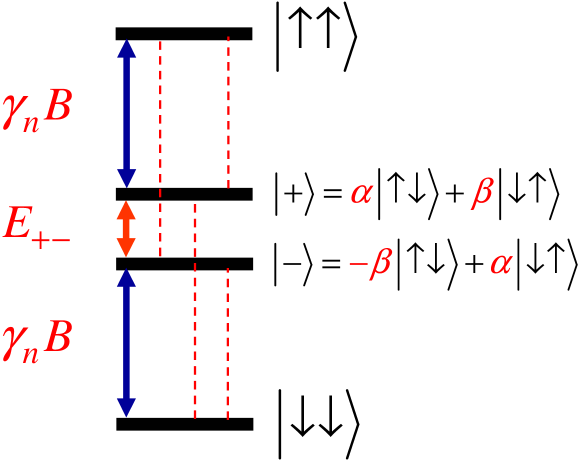
Figure 3: Energy levels for two nuclear spins coupled through the dipolar interaction. The flip-flop mechanism corresponds to transitions between the states $|+\rangle$ and $|-\rangle$, which are admixtures of $\mid\uparrow\downarrow\rangle$ and $\mid\downarrow\uparrow$ states. The anisotropic hyperfine interaction couples states differing by $\sim\gamma_{n}B$ in energy.

For now we assume the nuclear spins are unpolarized ($T=\infty$) so that $\langle\sum_{i}A_{i}I_{iz}\rangle=0$. This approximation will be relaxed below. The time dependent correlation function for nuclear spins is given by

$$S(t) = \left\langle\sum_{i}A_{i}I_{iz}(t)\sum_{j}A_{j}I_{jz}(0)\right\rangle$$ (75)

$$= \sum_{i}A_{i}^{2}\langle I_{iz}(t)I_{iz}(0)\rangle+\sum_{i,j(\neq i)}A_{i}A_{j}\langle I_{iz}(t)I_{jz}(0)\rangle.$$

We now invoke a “pair approximation” by assuming

$$\langle I_{iz}(t)I_{iz}(0)\rangle\approx\sum_{j(\neq i)}\langle I_{iz}(t)I_{iz}(0)\rangle_{ij},$$ (76)

$$\langle I_{iz}(t)I_{jz}(0)\rangle\approx\langle I_{iz}(t)I_{jz}(0)\rangle_{ij},$$ (77)

where $\langle\cdot\rangle_{ij}$ denotes a thermal average restricted to the $ij$ Hilbert space. The operator $I_{iz}(t)$ is in the Heisenberg representation defined by the two particle Hamiltonian Eq. (74). Plugging Eqs. (76) and (77) in Eq. (75) and reordering terms we get

$$S(t)\approx\sum_{i<j}\langle\hat{\eta}_{ij}(t)\hat{\eta}_{ij}(0)\rangle_{ij},$$ (78)

with

$$\hat{\eta}_{ij}=A_{i}I_{iz}+A_{j}I_{jz}.$$ (79)

The same derivation could be given for finite temperature, when the thermal average of the hyperfine field is non-zero. The result is identical to Eq. (78) except for the substitution $\hat{\eta}_{ij}\rightarrow\delta\hat{\eta}_{ij}=\hat{\eta}_{ij}-\langle\hat{\eta}_{ij}\rangle$. Using the definition of the noise spectrum [Eq. (6)] and expanding the correlator in the energy eigenstates of the pair Hamiltonian Eq. (74) we get

$$\tilde{S}_{ij}(\omega)=\sum_{\alpha,\beta}p_{\alpha}\left|\langle\alpha|\delta\hat{\eta}_{ij}|\beta\rangle\right|^{2}\delta\left(\omega-E_{\beta\alpha}\right),$$ (80)

with $E_{\beta\alpha}=E_{\beta}-E_{\alpha}$ the energy difference between the energy eigenstates $|\alpha\rangle,|\beta\rangle$, and $p_{\alpha}$ the (thermal) occupation of state $\alpha$. Therefore the noise spectrum is a sum over all possible transition frequencies induced by the operator $\hat{\eta}_{ij}$. For nuclear spin $1/2$ the $ij$ Hamiltonian has the following eigenenergies and eigenstates (See Fig. 3)

$$E_{\uparrow\uparrow} = \gamma_{n}B-b_{ij}+a_{ij},$$ (81)

$$E_{+} = b_{ij}+\sqrt{b_{ij}^{2}+\Delta_{ij}^{2}},$$ (82)

$$E_{-} = b_{ij}-\sqrt{b_{ij}^{2}+\Delta_{ij}^{2}},$$ (83)

$$E_{\downarrow\downarrow} = -\gamma_{n}B-b_{ij}-a_{ij},$$ (84)

$$|+\rangle = \cos{\frac{\theta}{2}}\mid\uparrow\downarrow\rangle+\sin{\frac{\theta}{2}}\mid\downarrow\uparrow\rangle,$$ (85)

$$|-\rangle = -\sin{\frac{\theta}{2}}\mid\uparrow\downarrow\rangle+\cos{\frac{\theta}{2}}\mid\downarrow\uparrow\rangle,$$ (86)

with

$$a_{ij} = \frac{1}{4}\left(A_{i}+A_{j}\right),$$ (87)

$$\Delta_{ij} = \frac{1}{4}\left(A_{i}-A_{j}\right),$$ (88)

$$\cos{\theta} = \frac{\Delta_{ij}}{\sqrt{b_{ij}^{2}+\Delta_{ij}^{2}}},$$ (89)

$$\sin{\theta} = \frac{b_{ij}}{\sqrt{b_{ij}^{2}+\Delta_{ij}^{2}}}.$$ (90)

Using Eqs. (85), (86) the transition matrix element is easily found to be

$$\langle-|\hat{\eta}_{ij}|+\rangle=-4\Delta_{ij}\sin{\frac{\theta}{2}}\cos{\frac{\theta}{2}}=-2\Delta_{ij}\sin{\theta}.$$ (91)

The transition frequency is simply the difference between Eqs. (82) and (83),

$$E_{+-}=2\sqrt{b_{ij}^{2}+\Delta_{ij}^{2}}.$$ (92)

The resulting noise spectrum is therefore

$$\tilde{S}_{ij}(\omega)=\left(A^{{\rm rms}}_{ij}\right)^{2}\delta(\omega)+4\frac{b_{ij}^{2}\Delta_{ij}^{2}}{b_{ij}^{2}+\Delta_{ij}^{2}}\left[p_{+}\delta(\omega+E_{+-})+p_{-}\delta(\omega-E_{+-})\right],$$ (93)

with a static contribution given by

$$\left(A^{{\rm rms}}_{ij}\right)^{2} = 4\left[\left(p_{\uparrow\uparrow}+p_{\downarrow\downarrow}\right)a_{ij}^{2}+\left(p_{+}+p_{-}\right)\frac{\Delta_{ij}^{4}}{b_{ij}^{2}+\Delta_{ij}^{2}}\right]$$ (94)

$$-4\left[\left(p_{\uparrow\uparrow}-p_{\downarrow\downarrow}\right)a_{ij}+\left(p_{+}-p_{-}\right)\frac{\Delta_{ij}^{2}}{\sqrt{b_{ij}^{2}+\Delta_{ij}^{2}}}\right]^{2}.$$

The free induction decay due to this noise spectrum can be easily calculated using Eq. (19) and the filter function Eq. (21),

$$\langle\langle\sigma_{+}(t)\rangle\rangle = \exp{\left[-\frac{1}{2}\sum_{i<j}\left(A^{{\rm rms}}_{ij}\right)^{2}t^{2}\right]}$$ (95)

$$\times \exp{\left[-2\sum_{i<j}\left(p_{+}+p_{-}\right)\frac{b_{ij}^{2}\Delta_{ij}^{2}}{b_{ij}^{2}+\Delta_{ij}^{2}}t^{2}{\rm sinc}^{2}\left(\sqrt{b_{ij}^{2}+\Delta_{ij}^{2}}t\right)\right]},$$

where $\rm{sinc}(x)=\sin{(x)}/x$. As expected, the FID decay is usually dominated by the zero-frequency noise amplitue $A^{{\rm rms}}_{ij}$ [Eq. (94)]. The dipolar-induced decay may be visible provided $A^{{\rm rms}}_{ij}$ is much smaller than the finite frequency noise amplitudes. For example, this is the case if the nuclear spins are polarized, since we have $A^{{\rm rms}}_{ij}=0$ exactly when $p_{\downarrow\downarrow}=1$ in Eq. (94).

The Hahn echo decay envelope is derived after integration with the filter function Eq. (22),

$$\langle\langle\sigma_{+}(2\tau)\rangle\rangle=\exp{\left[-8\sum_{i<j}\left(p_{+}+p_{-}\right)b_{ij}^{2}\Delta_{ij}^{2}\tau^{4}{\rm sinc}^{4}\left(\sqrt{b_{ij}^{2}+\Delta_{ij}^{2}}\tau\right)\right]}.$$ (96)

At $T\rightarrow\infty$ ($p_{+}=p_{-}=1/4$) Eq. (96) is identical to the echo decay obtained by two completely different methods, viz. the lowest order cluster expansion [Eq. (20) in Ref. witzel05 ] and the quasiparticle excitation model [Eq. (18) in Ref. yao05 ]. As expected, Eq. (96) is independent of zero-frequency noise, and is exactly equal to $1$ when either $b_{ij}=0$ or $\Delta_{ij}=0$, or when the nuclear spins are polarized ($p_{+}=p_{-}=0$).

By expanding the exponent in Eqs. (95) and (96) in powers of time, we find that only even powers are present. The short time behavior for FID is $\sim\textrm{e}^{-t^{2}}$, while for Hahn echo $\sim\textrm{e}^{-\tau^{4}}$. This short time approximation is valid for times much shorter than the inverse cut-off frequency of the noise spectrum obtained after summing over all pairs $i,j$.

4.2 Mean field theory of noise broadening: quasiparticle lifetimes

We showed that the noise spectrum due to flip-flop transitions in the Hilbert space formed by two nuclear spins $i,j$ is a linear combination of delta functions. We may extend this pair approximation to clusters larger than two, and the number of delta functions will grow exponentially with cluster size [This can be done by sistematically increasing the size of the Hilbert space beyond a single pair $i,j$ in Eqs. (76) and (77)]. These delta functions can be interpreted as well defined nuclear spin excitations with infinite lifetime. With this interpretation in mind, it is natural to expect that the many-body interactions of the pair $i,j$ with other nuclear spins will limit the lifetime of the flip-flop excitations, i.e., the delta functions will be broadened, see Fig. 4.

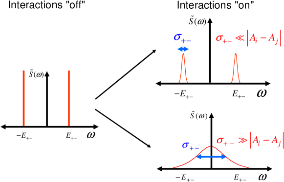
Figure 4: An isolated pair of nuclear spins with infinite lifetime will produce a sharp peak in the noise spectrum. The role of the many-body interactions with other nuclear spins is to broaden this peak and smooth out the noise spectrum for the collective nuclear spin excitations. Here we calculate the line broadening for each pair flip-flop transition using a procedure similar to van Vleck’s method of moments.

We can add broadening to the delta functions in a mean field fashion by using the method of moments, which is applicable at infinite temperature (no nuclear spin polarization, i.e. $k_{B}T\gg\gamma_{n}B$). In this limit, the noise spectrum is written as

$$\tilde{S}_{ij}(\omega)=\sum_{\alpha,\beta}\frac{1}{2^{N}}|\langle\alpha|\hat{\eta}_{ij}|\beta\rangle|^{2}\delta(\omega-E_{\beta\alpha}),$$ (97)

where here $\alpha,\beta$ denote exact many-body eigenstates of the system of $N$-coupled nuclear spins. The $n$-th moment $\int\omega^{n}\tilde{S}(\omega)d\omega$ can be calculated exactly using the invariance of the trace. Consider the zeroth-moment,

$$\int_{-\infty}^{\infty}\tilde{S}_{ij}(\omega)d\omega = \frac{1}{2^{N}}\sum_{\alpha,\beta}\langle\alpha|\hat{\eta}_{ij}|\beta\rangle\langle\beta|\hat{\eta}_{ij}|\alpha\rangle$$ (98)

$$=\frac{1}{2^{N}}\rm{Tr}\left\{\hat{\eta}_{ij}^{2}\right\}=\frac{1}{4}\left(A_{i}^{2}+A_{j}^{2}\right).$$

Accordingly, the second moment is given by

$$\int_{-\infty}^{\infty}\omega^{2}\tilde{S}_{ij}(\omega)d\omega = -\frac{1}{2^{N}}\rm{Tr}\left\{\left[{\cal H}_{eff}^{n},\hat{\eta}_{ij}\right]^{2}\right\}$$ (99)

$$= \frac{1}{2}A_{i}^{2}\sum_{k\neq i}b_{ik}^{2}-b_{ij}^{2}A_{i}A_{j}+\frac{1}{2}A_{j}^{2}\sum_{k\neq j}b_{jk}^{2}.$$

Note that Eqs. (98) and (99) are exact at infinite temperature.

The mean field approximation employed here assumes each delta function in the noise spectrum can be approximated by a Gaussian function normalized to one. The noise spectrum becomes

$$\tilde{S}_{ij}(\omega)\approx\sum_{\alpha,\beta}\frac{1}{4}|\langle\alpha|\hat{\eta}_{ij}|\beta\rangle|^{2}\frac{1}{\sqrt{2\pi\sigma_{\alpha\beta}^{2}}}\exp{\left[-\frac{(\omega-E_{\alpha\beta})^{2}}{2\sigma_{\alpha\beta}^{2}}\right]},$$ (100)

and the second moment is

$$\int_{-\infty}^{\infty}\omega^{2}\tilde{S}_{ij}(\omega)d\omega\approx\sum_{\alpha,\beta}\frac{1}{4}|\langle\alpha|\hat{\eta}_{ij}|\beta\rangle|^{2}\left(\sigma_{\alpha\beta}^{2}+E_{\alpha\beta}^{2}\right).$$ (101)

We now calculate the broadenings $\sigma_{\alpha\beta}$ by equating Eq. (101) with Eq. (99). This procedure can be carried out exactly, since the noise spectrum has two identical peaks (Fig. 4) at frequencies $\pm E_{+-}$. The broadening is found to be

$$\sigma_{+-}^{2}=\frac{b_{ij}^{2}+\Delta_{ij}^{2}}{4\Delta_{ij}^{2}b_{ij}^{2}}\sum_{k\neq i,j}\left(b_{ik}^{2}A_{i}^{2}+b_{jk}^{2}A_{j}^{2}\right).$$ (102)

When $\Delta_{ij}<\sim b_{ij}$, the broadening becomes of the same order of magnitude as van Vleck’s second moment for the dipolar interaction (equal to $9\sum_{k}b_{ik}^{2}$ slichter96 ). For $\Delta_{ij}\gg b_{ij}$ we have $\sigma_{+-}\sim\Delta_{ij}$, and $\sigma_{+-}/E_{+-}\sim 1$. This type of excitation is of high frequency and short lifetime, showing fast decay to a small loss of contrast as described by Eqs. (36), (38). The broadenings describe the diffusion of localized nuclear spin excitations (deviations from thermal equilibrium) over length scales greater than the pair distance.

By adding broadenings to the delta functions in Eq. (93) we are able to plot a smooth noise spectrum, and study the relative contributions of a large number of nuclear spins as a function of a continuous frequency. The modified Eq. (93) summed over all nuclear pair contributions reads

$$\tilde{S}(\omega) = 4\sum_{i<j}\frac{b_{ij}^{2}\Delta_{ij}^{2}}{b_{ij}^{2}+\Delta_{ij}^{2}}\left\{p_{+}\frac{\textrm{e}^{-\frac{(\omega-E_{+-})^{2}}{2\sigma^{2}_{+-}}}}{\sqrt{2\pi\sigma^{2}_{+-}}}+p_{-}\frac{\textrm{e}^{-\frac{(\omega+E_{+-})^{2}}{2\sigma^{2}_{+-}}}}{\sqrt{2\pi\sigma^{2}_{+-}}}\right\}$$ (103)

$$+\sum_{i<j}\left(A^{{\rm rms}}_{ij}\right)^{2}\delta(\omega).$$

For studies of echo decay we may drop the delta function contribution at zero frequency. Note that the first part of Eq. (103) gives an additional zero frequency contribution, that is the limit $\omega\rightarrow 0$ of the broadened spectrum.

5 Electron spin echo decay of a phosphorus impurity in silicon: Comparison with experiment

In this section we apply our theory to a phosphorus donor impurity in bulk silicon. We consider both natural samples ($f=4.67\%$ ²⁹Si nuclear spins) and isotopically enriched samples ($f=99.23\%$ ²⁹Si nuclear spins). We show explicit numerical calculations of the nuclear spin noise spectrum resulting from dipolar nuclear-nuclear couplings, predict the Hahn echo envelope and compare our results with the experimental data of Tyryshkin et al tyryshkin06 and Abe et al abe04 .

5.1 Effective mass model for a phosphorus impurity in silicon

Here the donor impurity is described within effective mass theory by a Kohn-Luttinger wave function kohn57 ,

$$\Psi({\mathbf{r}}) = \frac{1}{\sqrt{6}}\sum_{j=1}^{6}F_{j}({\mathbf{r}})u_{j}({\mathbf{r}})e^{i{\mathbf{k}_{j}\cdot r}},$$ (104)

$${\mathbf{k}_{j}} = 0.85\frac{2\pi}{a_{\rm{Si}}}\hat{k}_{j},\;\hat{k}_{j}\in\left\{\hat{x},-\hat{x},\hat{y},-\hat{y},\hat{z},-\hat{z}\right\},$$ (105)

$$F_{1,2}({\mathbf{r}}) = \frac{\exp{\left[-\sqrt{\frac{x^{2}}{(nb)^{2}}+\frac{y^{2}+z^{2}}{(na)^{2}}}\right]}}{\sqrt{\pi(na)^{2}(nb)}},$$ (106)

with envelope functions $F_{j}$ describing the effective mass anisotropies. Here $n=(0.029eV/E_{i})^{1/2}$ with $E_{i}$ being the ionization energy of the impurity ($E_{i}=0.044$ eV for the phosphorus impurity, hence $n=0.81$ in our case), $a_{\rm{Si}}=5.43$ Å the lattice parameter for Si, $a=25.09$ Å and $b=14.43$ Å characteristic lengths for Si hydrogenic impurities feher59a . Moreover, we will use experimentally measured values for the charge density on each Si lattice site $|u({\mathbf{R}_{i}})|^{2}=\eta\approx 186$ kohn57 . Hence the isotropic hyperfine interaction is given by

$$A^{\rm{iso}}_{i} = \frac{16\pi}{9}\gamma_{e0}\gamma_{n}\eta\left[F_{1}({\mathbf{R}_{i}})\cos{(k_{0}X_{i})}\right.$$ (107)

$$\left.+F_{3}({\mathbf{R}_{i}})\cos{(k_{0}Y_{i})}+F_{5}({\mathbf{R}_{i}})\cos{(k_{0}Z_{i})}\right]^{2},$$

with the Si conduction band minimum at $k_{0}=(0.85)2\pi/a_{\rm{Si}}$, gyromagnetic ratios for ²⁹Si nuclear spins $\gamma_{n}=5.31\times 10^{3}$ (sG)^-1, and the free electron $\gamma_{e0}=1.76\times 10^{7}$ (s G)^-1. It is instructive to check the experimental validity of Eq. (107) by calculating the inhomogeneous line-width $\sim 1/(\gamma_{e0}T_{2}^{*})$. A simple statistical theory [Eq. (58)] leads to

$$\langle\left(\omega/\gamma_{e0}-B\right)^{2}\rangle=\frac{f}{(2\gamma_{e0})^{2}}\sum_{{\mathbf{R}_{i}}\neq{\mathbf{0}}}\left(A^{\rm{iso}}_{i}\right)^{2}.$$ (108)

For natural silicon (nuclear spin fraction $f=0.0467$) our calculated root mean square line-width is equal to $0.89$ G. On the other hand, a simple spin resonance scan leads to $2.5$ G$/2\sqrt{2\ln{2}}=1.06$ G feher59a . Therefore the simple model employed here is able to explain 84% of the experimental hyperfine line-width. This is the level of agreement that we should expect when comparing our theory for echo decay with experiment.

5.2 Explicit calculations of the nuclear spin noise spectrum and electron spin echo decay of a phosphorus impurity in silicon

The nuclear spin noise spectrum is calculated from Eq. (103) by excluding the $\delta(\omega)$ contribution. For each pair $i,j$ we calculate the transition frequency Eq. (92) and broadening Eq. (102) using the derived microscopic values of the hyperfine interaction [Eq. (107)] and the dipolar interaction

$$b_{ij}=-\frac{1}{4}\gamma_{n}^{2}\hbar\frac{1-3\cos^{2}{\theta_{ij}}}{R_{ij}^{3}}.$$ (109)

For silicon the sites $i,j$ lie in a diamond lattice with parameter $a_{{\rm si}}=5.43$ Å. We wrote a computer program that sums over lattice sites ${\bm{R}}_{i}$ within $r_{0}$ of the center of the donor. Each site ${\bm{R}}_{i}$ is then summed with all sites ${\bm{R}}_{j}$ within $r^{\prime}_{0}$ of ${\bm{R}}_{i}$ (excluding double counting). After numerical tests we concluded that the values $r_{0}=200$ Å and $r^{\prime}_{0}=10$ Å were high enough to guarantee convergence (increasing $r_{0}$ and $r^{\prime}_{0}$ changes the calculations by a negligible amount). Our explicit numerical calculations for the echo decay without broadening [Eq. (96)] reproduced the equivalent calculation of Witzel et al. witzel05 with no visible deviation. For $k_{B}T\gg\gamma_{n}B$ we may assume that the nuclear spins are completely unpolarized (the experimental data was taken at $T=4$ K and $B=0.3$ T tyryshkin06 ). We account for the isotopic fraction $f$ (ratio of sites containing nuclear spin $1/2$) using a simple averaging method. For example, the pair populations are set as $p_{+}=p_{-}=f^{2}/4$, and the broadening $\sigma^{2}_{+-}\propto f$ [note $\sum_{k}b^{2}_{ij}$ in Eq. (102)].

Figure 5: Nuclear spin noise affecting the electron spin phase. We show the noise spectrum for several magnetic field orientation angles $\theta$ with respect to the (001) direction. As $\theta$ is increased from zero, a broad peak develops at a frequency close to the dipolar splitting between nearest neighbors in the lattice. In this case the noise spectrum is clearly non-monotonous, and cannot be described by a Markovian model. The spin echo envelope is a frequency integral of the noise spectrum weighted by a filter function.

Fig. 5 shows the nuclear spin noise spectrum for natural Si at four different magnetic field orientation angles $\theta$ with respect to the crystal direction (001). Here $\theta=0^{\circ}$ corresponds to $\bm{B}\parallel(001)$, while $\theta=90^{\circ}$ corresponds to $\bm{B}\parallel(110)$. For $\theta$ away from zero the noise spectrum is charaterized by a broad peak at which the flip-flop transition frequencies $E_{+-}$ accumulate. The fact that the spectrum is non-monotonic implies important non-Markovian behavior for electron spin dynamics (recall that a Markovian noise spectrum is defined as a sum of Lorentzians, hence it is always monotonic). Interestingly, for $\theta$ close to zero and at low frequencies ($\omega<5\times 10^{3}$ s^-1), the spectrum appears to be similar to a Lorentzian peaked at $\omega=0$ However, one can not fit a Lorentzian up to high frequencies because the assymptotic behavior deviates significantly from $1/\omega^{2}$.

Figure 6: Electron spin echo decay of a phosphorus impurity in natural silicon (4.67% ²⁹Si nuclear spins) for two different magnetic field orientations. We show experimental data from Ref. tyryshkin06 together with theoretical calculations without flip-flop broadening (identical to Ref. witzel05 ) and with flip-flop broadening. The latter is calculated by directly integrating the noise spectrum shown in Fig. 5 with the appropriate filter function.

The Hahn echo is obtained by integrating the noise spectrum multiplied by the filter function Eq. (22) up to a frequency cut-off $\Lambda$ (we used $\Lambda=10^{6}-10^{7}$ s^-1, and $df\sim 1-10$ s^-1 in our numerical calculations). The result is shown in Fig. 6 for two different orientations. We show calculations of the echo without broadening [Eq. (96), identical to the result shown in Ref. witzel05 ] and for the echo with broadening, that is obtained through direct integration of the noise spectrum shown in Fig. 5. Note that the two theories are in close agreement here because for low nuclear spin density ($f=0.0467$) the broadenings are generally much smaller than the transition frequencies $E_{+-}$, at least for the important pairs causing spectral diffusion. Recall that our theory does not account for the anisotropic hyperfine interactions. Therefore our theoretical results should be compared to the monotonic envelope enclosing the experimental data points. The echo modulations due to the anisotropic hyperfine interaction is clearly visible at short times in the experimental data shown in Fig. 6. These oscillations produce a loss of contrast of about 10% at the short time regime. Apart from this effect, the agreement between theory and experiment is quite good.

Figure 7: Electron spin echo decay of a phosphorus impurity in isotopically enriched silicon (99.23% of ²⁹Si). Experimental data from Ref. abe04 .

Fig. 7 shows echo decay results for isotopically enriched samples ($f=99.23\%$). The experimental data is from Abe et al. abe04 . Note that here the echo modulations are very evident, the loss of contrast reaches $\sim 100\%$. The monotonic envelope on top of the experimental data is in reasonable agreement with the theory without broadening. However, the theory with broadening decays significantly faster. The difference between both theories increases for increasing $f$. This suggests that the mean-field theory proposed in section 4.2 overestimates the broadening. The author expects that a more sophisticated many-body calculation may account for this discrepancy.

Fig. 8 shows the dependence of the $1/e$ echo decay time ($T_{2}$) with the magnetic field angle. The shortest value of $T_{2}$ is obtained when $\bm{B}$ is along the (111) direction ($\theta=54.74^{\circ}$). In this case none of the nearest neighbor pairs have zero dipolar couplings. Only pairs $i,j$ with $\bm{R}_{ij}$ parallel to the (100), (010), and (001) directions have their dipolar interaction turned off by the magic angle [$\theta_{ij}=54.74^{\circ}$ implies $\cos{\theta_{ij}}=1/\sqrt{3}$ and $b_{ij}=0$, see Eq. (109)]. On the other hand for $\bm{B}\parallel(001)$, $T_{2}$ is longer by a factor of three. This occurs because the nearest neighbor pairs, that usually give the strongest contribution to echo decay, are forming a magic angle with respect to $\bm{B}\parallel(001)$.

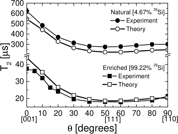
Figure 8: Orientation dependence of the 1/e echo decay time $T_{2}$. $\theta$ is the angle between the applied magnetic field and the crystalographic (001) direction, so that $\theta=90^{\circ}$ is along the (110) direction. We show experimental data for natural Si tyryshkin06 and for isotopically enriched Si abe04 . The theoretical calculations shown are without broadening. For natural Si, the experimental data was corrected for a $\theta$ independent instantaneous diffusion decay, see Ref. tyryshkin06 . Because of this the theoretical $T_{2}$’s are lower than the experimental $T_{2}$’s reported in Ref. tyryshkin06 , in contrast to what is observed in Fig. 6.

We now discuss the time dependence of the echo envelope. The echo decay without broadening fits well to the expression

$$\langle\sigma_{+}(2\tau)\rangle=\textrm{e}^{-\left(\frac{2\tau}{T_{2}}\right)^{2.3}}$$ (110)

for a wide range of $2\tau$ centered around $T_{2}$ and for all values of $f$ (for a log-log plot, see Fig. 9 of Ref. witzel06 ). Tyryshkin et al. tyryshkin06 studied the time dependence of the natural silicon experimental data by fitting the expression $v_{E}(2\tau)=\textrm{e}^{-2\tau/T^{\prime}_{2}}\textrm{e}^{-(2\tau/T_{2})^{n}}$. Here $T^{\prime}_{2}$ was interpreted as arising from a combination of spin-flip processes and the instantaneous diffusion mechanism, due to the finite concentration of donors. Tyryshkin et al. reported $T^{\prime}_{2}=1.1$ ms and exponent $n=2.4\pm 0.1$ for all sample orientation angles between $20^{\circ}\leq\theta\leq 90^{\circ}$. For $\theta=10^{\circ}$ they found $n=2.6\pm 0.1$, while for $\theta=0^{\circ}$ $n=3.0\pm 0.2$. The time dependence at angles close to the (001) direction is yet to be explained theoretically. At natural abundance ($f=0.0467$) the theory with broadening and the theory without broadening have similar time dependences. However, as $f$ increases the time dependence of the broadened theory deviates significantly from the theory without broadening. As an example, for $f=0.9923$ and $\theta=50^{\circ}$ the broadened theory shows a cross-over from $\textrm{e}^{-\tau^{3.3}}$ at short $\tau<3$ $\mu$s to $\textrm{e}^{-\tau^{1.7}}$ for $\tau>3$ $\mu$s. This indicates that adding broadening to the nuclear spin excitations leads to observable effects in the time dependence of electron spin coherence. Unfortunately, the echo modulations are too strong in isotopically enriched samples (Fig. 7). This makes the precise experimental determination of the time dependence of the echo envelope quite difficult.

Eq. (110) allows us to extract scaling of the 1/e decay time $T_{2}$ with the nuclear spin fraction $f$. Note that in the theory without broadening $f$ appears as a pre-factor in the exponent due to $p_{+}+p_{-}=f^{2}/4$. Therefore we have simply

$$T_{2}\propto f^{-2/2.3}=f^{-0.87}.$$ (111)

Abe et al. abe06 measured $T_{2}$ for seven isotopically engineered samples with $f$ ranging from 0.2%–100%. Their study shows that $T_{2}$ must scale between $f^{-0.86}$ and $f^{-0.89}$ in good agreement with Eq. (111).

It is interesting to study the number and location of nuclear spins contributing to the noise spectrum. Fig. 9 shows the contribution due to pairs inside shells concentric at the donor center (for natural silicon and $\theta=50^{\circ}$). The contribution for $r_{0}<50$ Å  is quite small, but extends over a wide frequency spectrum. These nuclear spins are said to form a “frozen core”, because their noise amplitude is suppressed due to the strong difference in hyperfine fields affecting sites $i,j$. The frozen core of a Si:P donor has about $3\times 10^{4}$ nuclear spins. This frozen core effect plays an important role in other contexts as well such as optical spectroscopy experiments devoe81 . The nuclear spin noise theory developed here allows a quantitative description of this effect. From Fig. 9 it is evident that a significant fraction of the finite frequency noise power comes from the large number of nuclear spins located between $50$ Å  and $100$ Å  off the donor center (about $\sim 2\times 10^{5}$ nuclear spins). These pairs are satisfying a quasi-resonance condition $\Delta_{ij}\sim b_{ij}$.

Figure 9: Contribution of nuclear spins located at concentric shells around the donor (natural Si, $\theta=50^{\circ}$). Nuclear pairs closer to the center ($r_{0}<50$ Å) have their fluctuation amplitude suppressed by the strong hyperfine field difference between sites $i,j$, forming a frozen core. The largest contribution is due to pairs located at $50$ Å $<r_{0}<$ $100$ Å.

6 Conclusions and outlook for the future

In this chapter we described the coherent evolution of an electron spin subject to time dependent fluctuations along its quantization axis. We showed that in the Gaussian approximation the electron spin transverse magnetization can be expressed as a frequency integral over the magnetic noise spectrum multiplied by an appropriate filter function. The filter function depends on the particular pulse sequence used to probe spin coherence, differing substantially at low frequencies for free induction decay (FID) and Hahn echo. For a Gauss-Markov model (Lorentzian noise spectrum centered at zero frequency) we showed that the short time decay of the FID signal is approximately $\textrm{e}^{-t^{2}}$, while the echo decays according to $\textrm{e}^{-\tau^{3}}$.

We applied this general relationship between noise and decoherence to the case of a localized electron spin in isotopically engineered silicon, where the magnetic noise is mainly due to the dipolar fluctuation of spin-1/2 lattice nuclei. The nuclear spin noise spectrum was calculated from a pair-flip-flop model, resulting in a linear combination of sharp transitions (delta functions). The echo decay due to these sharp transitions is identical to the one derived by the lowest order cluster expansion witzel05 . Next, we showed how to obtain a smooth noise spectrum by adding broadening to these transitions using a mean-field approach. The resulting noise spectrum was found to be strongly non-monotonic, hence qualitatively different from the usual Lorentzian spectrum of a Gauss-Markov model. This structured noise spectrum is able to explain the non-Markovian dynamics ($\sim\textrm{e}^{-\tau^{2.3}}$) observed in electron spin echo experiments for phosphorus doped silicon. We compared the theories with and without broadening to two sets of experimental data, for natural and isotopically enriched silicon. The agreement was quite good for natural silicon, but not as good for ²⁹Si enriched samples.

It is interesting to compare our results to the set of non-Gaussian phenomenological theories proposed a long time ago by Klauder and Anderson klauder62 . These authors classified spectral diffusion behavior in two groups, depending on the nature of the interactions causing magnetic noise. In “$T_{1}$ samples” the magnetic noise is caused by non-resonant spins fluctuating individually (e.g., due to phonon emission). On the other hand the magnetic noise at “$T_{2}$ samples” is caused by the mutual interaction of the non-resonant spins (For example, a nuclear spin bath weakly coupled to the lattice is a “$T_{2}$ sample” because the longitudinal nuclear spin relaxation time $T^{n}_{1}$ is much longer than the transverse relaxation time $T^{n}_{2}$). Klauder and Anderson showed that echo decay behavior in a variety of $T_{1}$ samples could be described by a Markovian theory by making assumptions about the general shape of the distribution of fluctuations at any given time. While a Gauss-Markov model leads to echo decay of the form $\sim\textrm{e}^{-\tau^{3}}$, a Lorentz-Markov model leads to $\textrm{e}^{-\tau^{2}}$ behavior, and intermediate non-Gaussian distributions result in $\textrm{e}^{-\tau^{n}}$ with $n$ between two and three. Later, Zhidomirov and Salikhov zhidomirov69 showed that similar behavior can be obtained in $T_{1}$ samples composed of a dilute distribution of magnetic impurities fluctuating according to a random telegraph noise model (Markovian with a non-Gaussian distribution).

Nevertheless the problem of echo decay behavior in “$T_{2}$ samples” remained open. It was found empirically by many authors (see chiba72 and references therein) that echo decay behavior in “$T_{2}$ samples” is usually well fitted to the expression $\sim\textrm{e}^{-\tau^{2}}$, and the Lorentz-Markov model of Klauder and Anderson was often invoked as a phenomenological explanation. Here we show that this behavior can be derived microscopically from a Gaussian model that takes into account the non-Markovian evolution of the coupled nuclear spin bath. The resulting behavior found by us [$\textrm{e}^{-\tau^{2.3}}$] is not due to a short time approximation [the short time behavior for each pair is actually given by $\textrm{e}^{-\tau^{4}}$, see Eq. (96)]. In order to explain these experiments we must consider the collective finite time evolution of a large number of nuclear spins [note that the characteristic frequency of fluctuation for a pair flip-flop $E_{+-}=2\sqrt{b_{ij}^{2}+\Delta_{ij}^{2}}$ gets renormalized to values much larger than the dipolar interaction $b_{ij}$ when the nuclear spins are subject to strong hyperfine inhomogeneities $\Delta_{ij}=(A_{i}-A_{j})/4$]. This theoretical explanation opens the way to novel microscopic interpretations of a series of pulse electron spin resonance experiments, where the electron spin may be viewed as a spectrometer of low frequency magnetic noise due to a large number of nuclear spins or other magnetic moments. For example, a recent experiment schenkel06 revealed that magnetic noise from the surface must play a role on spin echo decay of antimony impurities implanted in isotopically purified silicon (with a very low density of ²⁹Si nuclear spins in the bulk).

There are many open questions that deserve further investigation. First, what is the contribution of higher order nuclear spin transitions to the noise spectrum? This question may be answered by going beyond the simple pair flip-flop model assumed here, in a similar fashion as the cluster expansion developed in witzel05 , or using an alternative linked cluster expansion for the spin Green’s function saikin06 . Another interesting open question is the design of optimal sequences for suppressing the effects of nuclear spin noise in electron spin evolution, as was done for the random telegraph noise model in Ref. mottonen06 . This is particularly important in the context of spin-based quantum computation. The efficiency of a Carr-Purcell sequence in suppressing the electron spin coherence decay due to a nuclear spin bath was considered both in the framework of a semiclassical model (see Ref. desousa05 , where the role of nuclear spins greater than 1/2 was also considered) and using a cluster expansion approach witzel06b . Recently, it was shown that the electron mediated inter-nuclear coupling [Eq. (70)] may be exploited in order to recover electron spin coherence lost for the nuclear spin bath yao06 . We will certainly see many other interesting developments in the near future.

Acknowledgements

This research project began in 2001 in collaboration with Sankar Das Sarma, my Ph.D. advisor. I am grateful for and appreciate his guidance and support. The collaboration continued with Wayne Witzel, another Ph.D. student in S. Das Sarma’s group. This part of the work was supported by ARDA, US-ARO, US-ONR, and NSA-LPS. My postdoctoral work on this problem was in collaboration with K. Birgitta Whaley and Neil Shenvi. Neil also dedicated part of his Ph.D. thesis on problems related to electron spin dynamics due to nuclear spins. This part of the work was supported by the DARPA SPINS program and the US-ONR. My long, energetic and prolific collaboration with Neil and Wayne cannot be overstated. I acknowledge great discussions with J. Fabian, X. Hu, A. Khaetskii, D. Loss, L.J. Sham, L.M.K. Vandersypen, and I. Zutíc. The role of experimentalists in the development of this theory was also very important. I wish to thank Stephen Lyon, Alexei Tyryshkin, Thomas Schenkel, Kohei Itoh, and Eisuke Abe for discussions and for providing their experimental data before it was published. Finally, I wish to acknowledge an enlightening conversation with Professor Erwin Hahn, who kindly shared his astonishing intuition on the problems that he pioneered a long time ago.

References

- (1) A. Schweiger, G. Jeschke: Principles of Pulse Electron Paramagnetic Resonance (Oxford University Press, U.K. 2001)
- (2) X. Hu: Spin-based quantum dot quantum computing, in W. Pötz, U. Hohenester, J. Fabian (Eds.): Lecture Notes in Physics vol. 689 (Springer Berlin 2006); S. Das Sarma, R. de Sousa, X. Hu, B. Koiller: Solid State Commun. 133, 737 (2005)
- (3) F. Jelezko et al.: Phys. Rev. Lett. 92, 0764401 (2004)
- (4) J.M. Elzerman et al.: Nature 430, 431 (2004)
- (5) M. Xiao et al.: Nature 430, 435 (2004)
- (6) D. Rugar et al.: Nature 430, 329 (2004)
- (7) J. R. Petta et al.: Science 309, 2180 (2005)
- (8) G. Feher and E.A. Gere: Phys. Rev. 114, 1245 (1959)
- (9) H. Hasegawa: Phys. Rev. 118, 1523 (1960); L.M. Roth: Phys. Rev. 118, 1534 (1960)
- (10) R. de Sousa, S. Das Sarma: Phys. Rev. B 68, 155330 (2003)
- (11) M. Chiba, A. Hirai: J. Phys. Soc. Japan 33, 730 (1972)
- (12) B. Herzog, E.L. Hahn: Phys. Rev. 103, 148 (1956)
- (13) J.P. Gordon, K.D. Bowers: Phys. Rev. Lett. 1, 368 (1958)
- (14) J.R. Klauder, P.W. Anderson: Phys. Rev. 125, 912 (1962)
- (15) W.B. Mims: Electron spin echoes, in S. Geschwind (Ed.): Electron spin resonance (Plenum Press, NY, 1972); K. M. Salikhov, Yu. D. Tsvetkov: Electron Spin Echoes and its applications, in L. Kevan, R.N. Schwartz (Eds.): Time domain electron spin resonance (Wiley, NY 1979)
- (16) R. de Sousa, S. Das Sarma: Phys. Rev. B 68, 115322 (2003)
- (17) A.M. Tyryshkin, S.A. Lyon, A.V. Astashkin, A.M. Raitsimring: Phys. Rev. B 68, 193207 (2003)
- (18) A.M. Tyryshkin, J.J.L. Morton, S.C. Benjamin, A. Ardavan, G.A.D. Briggs, J.W. Ager, S.A. Lyon: J. Phys.: Condens. Matter 18, S783 (2006)
- (19) E. Abe, K.M. Itoh, J. Isoya, S. Yamasaki, Phys. Rev. B 70, 033204 (2004)
- (20) A. Ferretti, M. Fanciulli, A. Ponti, A. Schweiger: Phys. Rev. 72, 235201 (2005).
- (21) W.M. Witzel, R. de Sousa, S. Das Sarma: Phys. Rev. B 72, 161306(R) (2005)
- (22) W.M. Witzel, S. Das Sarma: Phys. Rev. B 74, 035322 (2006)
- (23) C.P. Slichter: Principles of Magnetic Resonance, 3rd edn. (Springer, Berlin 1996)
- (24) S. Saikin, L. Fedichkin: Phys. Rev. B 67, 161302(R) (2003)
- (25) N. Shenvi, R. de Sousa, K.B. Whaley: Phys. Rev. B 71, 224411 (2005)
- (26) I.A. Merkulov, Al.L. Efros, M. Rosen: Phys. Rev. B 65, 205309 (2002)
- (27) A.V. Khaetskii, D. Loss, L. Glazman: Phys. Rev. Lett. 88, 186802 (2002)
- (28) C. Deng, X. Hu: Phys. Rev. B 73, 241303(R) (2006)
- (29) D. Gammon et al.: Phys. Rev. Lett. 86, 5176 (2001); K. Ono, S. Tarucha: Phys. Rev. Lett. 92, 256803 (2004); P.-F. Braun et al.: Phys. Rev. Lett. 94, 116601 (2005); M.V.G. Dutt et al.: Phys. Rev. Lett. 94, 227403 (2005); F.H.L. Koppens: Science 309, 1346 (2005); A.C. Johnson et al.: Nature 435, 925 (2005)
- (30) N. Shenvi, R. de Sousa, K.B. Whaley: Phys. Rev. B 71, 144419 (2005)
- (31) W. Yao, R.-B. Liu, L.J. Sham: Phys. Rev. B 74, 195301 (2006)
- (32) W. Kohn: Shallow Impurity States in Silicon and Germanium, in F. Seitz, D. Turnbull (Eds.): Solid State Physics vol. 5, p. 257v (Academic Press, NY 1957)
- (33) G. Feher: Phys. Rev. 114, 1219 (1959)
- (34) E. Abe, A. Fujimoto, J. Isoya, S. Yamasaki, K.M. Itoh: cond-mat/0512404 (unpublished)
- (35) R.G. DeVoe, A. Wokaun, S.C. Rand, R. G. Brewer: Phys. Rev. B 23, 3125 (1981)
- (36) G.M. Zhidomirov, K.M. Salikhov: Sov. Phys. JETP 29 1037 (1969)
- (37) T. Schenkel et al.: Appl. Phys. Lett. 88, 112101 (2006)
- (38) R. de Sousa, N. Shenvi, K.B. Whaley: Phys. Rev. B 72, 045330 (2005)
- (39) S.K. Saikin, W. Yao, L.J. Sham: cond-mat/0609105
- (40) M. Möttönen, R. de Sousa, J. Zhang, K.B. Whaley: Phys. Rev. A 73, 022332 (2006)
- (41) W.M. Witzel, S. Das Sarma: cond-mat/0604577
- (42) W. Yao, R.-B. Liu, L.J. Sham: cond-mat/0604634