Magnetization of ballistic quantum dots
induced by a linear-polarized microwave field

Abstract

On a basis of extensive analytical and numerical studies we show that a linear-polarized microwave field creates a stationary magnetization in mesoscopic ballistic quantum dots with two-dimensional electron gas being at a thermal equilibrium. The magnetization is proportional to a number of electrons in a dot and to a microwave power. Microwave fields of moderate strength create in a one dot of few micron size a magnetization which is by few orders of magnitude larger than a magnetization produced by persistent currents. The effect is weakly dependent on temperature and can be observed with existing experimental techniques. The parallels between this effect and ratchets in asymmetric nanostructures are also discussed.

1 Introduction

Since 1990, when magnetization of an ensemble of $10^{7}$ mesoscopic rings had been detected experimentally levy1990 , the problem of magnetization of quantum dots of two-dimensional electron gas (2DEG) or persistent currents attracted a great deal of attention (see e.g. imry ; gilles and Refs. therein). It is well known that a magnetic field gives no magnetization in a classical system at thermal equilibrium (see e.g. mayer ). Thus, the persistent currents have a quantum origin and are relatively weak corresponding to values of one electron current of typical strength $3\times{10}^{-3}ev_{F}/L_{p}$ levy1990 where $v_{F}$ is the Fermi velocity and $L_{p}$ is a perimeter of quantum dot. Due to that skillful experimental efforts had been required to detect persistent currents of strength $I_{0}=ev_{F}/L_{p}$ in an isolated ballistic ring mailly .

The effects of ac-field on magnetization of mesoscopic dots have been discussed in kravtsov1993 ; kravtsov2005 . It was shown that ac-driving induces persistent currents which strength oscillates with magnetic flux. The amplitude of the current is proportional to the intensity of microwave field but still its amplitude is small compared to one electron current $ev_{F}/L_{p}$. Such currents have pure quantum origin and are essentially given only by one electron on a quantum level near the Fermi level. Experimental investigations of magnetization induced by ac-driving have been reported in bouchiat1 ; bouchiat2 . The amplitude of induced currents was in a qualitative agreement with the theoretical predictions kravtsov1993 ; kravtsov2005 . However, the strength of currents in one ring was rather weak (less than $nA$) and it was necessary to use an ensemble of ${10}^{5}$ rings to detect induced magnetization.

In this work we show that a liner-polarized microwave field generates strong orbital currents and magnetization in ballistic quantum dots. The magnetization (average non-zero momentum) of a dot is proportional to the number of electrons inside the dot and to the intensity of microwave field. The sign of magnetization depends on orientation of polarization in respect to symmetry axis of the dot. It is assumed that without microwave field the dot is in a thermal equilibrium characterized by the Fermi-Dirac distribution with a temperature $T$. A microwave field drives the system to a new stationary state with non-zero stationary magnetization to which contribute all electrons inside the dot. The steady state appears as a result of equilibrium between energy growth induced by a microwave field and relaxation which drives the system to thermal equilibrium. In contrast to the persistent currents discussed in imry ; gilles ; kravtsov2005 the dynamical magnetization effect discussed here has essentially classical origin and hence it gives much stronger currents. However, it disappears in the presence of disorder when the mean free path becomes smaller than the size of the dot. Thus the electron dynamics should be ballistic inside the dot which should have a stretched form since the effect is absent inside a ring and is weak inside a square shaped dot. Also the effect is most strong when the microwave frequency is comparable with a frequency of electron oscillations inside the dot. The above conditions were not fulfilled in the experiments bouchiat1 ; bouchiat2 and therefor the dynamical magnetization had not be seen there.

The physical origin of dynamical magnetization can be seen already from a simple model of two decoupled dissipative oscillators for which a monochromatic driving leads to a certain degree of synchronization with the driving phase pikovsky . This phenomenological approach was proposed by Magarill and Chaplik chaplik who gave first estimates for photoinduced magnetism in ballistic nanostructures. Here we develop a more rigorous approach based on the density matrix and semiclassical calculations of dynamical magnetization. We also extend our analysis to a generic case of enharmonic potential inside the dot that leads to qualitative changes in the magnetization dependence on microwave frequency. We also trace certain parallels between dynamical magnetization, directed transport (ratchets) induced by microwave fields in asymmetric nanostructures ratchet1 ; ratchet2 ; alik ; entin and the Landau damping landau ; pitaevsky .

The paper has the following structure: in Section II we consider the case of a quantum dot with harmonic potential, enharmonic potential is analyzed in Section III, a quantum dot in a form of Bunimovich stadium bunimovich is considered in Section IV, discussions and conclusions are given in Section V.

2 Quantum dots with a harmonic potential

Electron dynamics inside a two-dimensional (2D) dot is described by a Hamiltonian

$$H=(p_{x}^{2}+p_{y}^{2})/2m+U(x,y)-xf_{x}\cos\omega t-yf_{y}\cos\omega t$$ (1)

where $m$ is electron mass and $p_{x,y}$ and $x,y$ are conjugated momentum and coordinate. An external force $f_{x,y}$ is created by a linear-polarized microwave field with frequency $\omega$. The polarization angle $\theta$ and the force amplitude $f$ are defined by relations $f_{x}=f\cos\theta$, $f_{y}=f\sin\theta$. In this Section we consider the case of a harmonic potential $U(x,y)=m(\omega_{x}^{2}x^{2}+\omega_{y}^{2}y^{2})/2$ where $\omega_{x,y}$ are oscillation frequencies in $x,y$ directions (generally non equal).

Let us consider first a phenomenological case when an electron experiences an additional friction force $\bf{F}=-\gamma{\bf p}$ where $\gamma$ is a relaxation rate (this approach had been considered in chaplik and we give it here only for completeness). The dynamical equations of motion in this case are linear and can be solved exactly that gives at $t\gg 1/\gamma$:

$$\begin{array}[]{ll}x(t)=\Re\frac{e^{i\omega t}f_{x}/m}{\omega_{x}^{2}-\omega^{2}+i\gamma\omega}=\Re\;X(t),\\ y(t)=\Re\frac{e^{i\omega t}f_{y}/m}{\omega_{y}^{2}-\omega^{2}+i\gamma\omega}=\Re\;Y(t),\end{array}$$ (2)

where $\Re$ marks the real part. Then, the electron velocities are

$$\begin{array}[]{ll}x(t)=\Re\frac{ie^{i\omega t}\omega f_{x}/m}{\omega_{x}^{2}-\omega^{2}+i\gamma\omega}=\Re\;X(t),\\ y(t)=\Re\frac{ie^{i\omega t}\omega f_{y}/m}{\omega_{y}^{2}-\omega^{2}+i\gamma\omega}=\Re\;Y(t).\end{array}$$ (3)

This gives the average momentum

$$L=m\left\langle x(t)v_{y}(t)-y(t)v_{x}(t)\right\rangle=$$

$$\Re\frac{-i\omega f_{x}f_{y}/m}{(\omega_{x}^{2}-\omega^{2}+i\gamma\omega)(\omega_{y}^{2}-\omega^{2}-i\gamma\omega)}\quad.$$ (4)

In the limit of small $\gamma\ll\omega_{x,y}$ Eq.(4) gives for the off-resonance case

$$L_{off}=\frac{\gamma\omega^{2}(\omega_{x}^{2}-\omega_{y}^{2})f_{x}f_{y}/m}{(\omega_{x}^{2}-\omega^{2})^{2}(\omega_{y}^{2}-\omega^{2})^{2}},$$ (5)

while at the resonance $\omega=\omega_{x}$

$$L_{res}=\frac{f_{x}f_{y}/m}{\gamma(\omega_{x}^{2}-\omega_{y}^{2})}.$$ (6)

From a physical viewpoint an average momentum appears due to a phase shift between oscillator phases induced by dissipation and an orbit takes an elliptic form with rotation in one direction. In some sense, due to dissipation the two oscillators become synchronized by external force pikovsky . As usual mayer , an average orbital momentum $L$ for one electron gives a total magnetic moment $M=NLe/2mc$ where $N$ is a number of electrons in a quantum dot. A pictorial view of spectral dependence of $M$ on $\omega$ at various ratios $\omega_{x}/\omega_{y}$ is given in chaplik .

To extend the phenomenological approach described above we should take into account that the electrons inside the dot are described by a thermal distribution and the effects of microwave field should be considered in the frame of the Kubo formalism for the density matrix (see e.g. gilles ). For analysis it is convenient to use creation, annihilation operators defined by usual relations ${\hat{x}}=\sqrt{\frac{\hbar}{2m\omega_{x}}}({\hat{a}}+{\hat{a}}^{+})$, ${\hat{y}}=\sqrt{\frac{\hbar}{2m\omega_{y}}}({\hat{b}}+{\hat{b}}^{+})$ and ${\hat{p}}_{x}=-i\sqrt{\frac{m\hbar\omega_{x}}{2}}({\hat{a}}-{\hat{a}}^{+})$, ${\hat{p}}_{y}=-i\sqrt{\frac{m\hbar\omega_{y}}{2}}({\hat{b}}-{\hat{b}}^{+})$. The unperturbed Hamiltonian in absence of microwave field takes the form ${\hat{H}}_{0}=\hbar\omega_{x}({\hat{a}}^{+}{\hat{a}}+1/2)+\hbar\omega_{y}({\hat{b}}^{+}{\hat{b}}+1/2)$. Then the orbital momentum is

$${\hat{L}}=\frac{i\hbar}{2\sqrt{\omega_{x}\omega_{y}}}[(\omega_{x}-\omega_{y})({\hat{a}}{\hat{b}}-{\hat{a}}^{+}{\hat{b}}^{+})+$$

$$(\omega_{x}+\omega_{y})({\hat{a}}{\hat{b}}^{+}-{\hat{a}}^{+}{\hat{b}})].$$ (7)

The only non zero matrix elements of ${\hat{L}}$ are

$$<n_{x},n_{y}|{\hat{L}}|n_{x}+\delta_{x},n_{y}+\delta_{y}>=$$

$$\quad\frac{i\hbar}{2\sqrt{\omega_{x}\omega_{y}}}(\delta_{x}\omega_{x}-\delta_{y}\omega_{y})\times$$

$$\quad[(n_{x}+(1+\delta_{x})/2)(n_{y}+(1+\delta_{y})/2)]^{1/2},$$ (8)

where $\delta_{x,y}=\pm 1$ and $n_{x,y}$ are oscillator level numbers. The perturbation induced by a microwave field ${\hat{V}}(t)=(-f_{x}{\hat{x}}-f_{y}{\hat{y}})\cos\omega t={\hat{V}}\cos\omega t$ should be also expressed via operators ${\hat{a}},{\hat{a}}^{+},{\hat{b}},{\hat{b}}^{+}$.

In the Kubo formalism the evolution of the density matrix ${\hat{\rho}}(t)$ is described by the equation

$$\begin{array}[]{ll}i\hbar\frac{\partial{\hat{\rho}}}{\partial t}=[{\hat{H}}_{0}+{\hat{V}}(t),{\hat{\rho}}]-i\hbar\gamma({\hat{\rho}}-{\hat{\rho}}_{0})\end{array}$$ (9)

where ${\hat{\rho}}_{0}$ is the equilibrium density matrix:
${\hat{\rho}}_{0}=\sum_{n_{x},n_{y}\geq 0}\rho_{n_{x},n_{y}}|n_{x},n_{y}><n_{x},n_{y}|$. Using perturbation theory ${\hat{\rho}}(t)$ can be expanded in powers of the external potential amplitude ${\hat{V}}(t)$ : ${\hat{\rho}}(t)={\hat{\rho}}_{0}+{\hat{\rho}}_{1}(t)+{\hat{\rho}}_{2}(t)+...$. In the first order we have

$$<\alpha|{\hat{\rho}}_{1}(t)|\beta>=\frac{(\rho(\epsilon_{\beta})-\rho(\epsilon_{\alpha}))<\alpha|V|\beta>}{\epsilon_{\beta}-\epsilon_{\alpha}-\hbar\omega+i\gamma\hbar}e^{i\omega t}/2+$$

$$\frac{(\rho(\epsilon_{\beta})-\rho(\epsilon_{\alpha}))<\alpha|V|\beta>}{\epsilon_{\beta}-\epsilon_{\alpha}+\hbar\omega+i\gamma\hbar}e^{-i\omega t}/2\quad.$$ (10)

For the harmonic potential we obtain

$$<n_{x}+\delta_{x},n_{y}|{\hat{\rho}}_{1}(t)|n_{x},n_{y}>=$$

$$(\rho_{n_{x},n_{y}}-\rho_{n_{x}+\delta_{x},n_{y}})f_{x}\sqrt{\frac{n_{x}+(1+\delta_{x})/2}{8\hbar m\omega_{x}}}\times$$

$$\left(\frac{e^{i\omega t}}{-\omega_{x}\delta_{x}-\omega+i\gamma}+\frac{e^{-i\omega t}}{-\omega_{x}\delta_{x}+\omega+i\gamma}\right)\;,$$

$$<n_{x},n_{y}+\delta_{y}|{\hat{\rho}}_{1}(t)|n_{x},n_{y}>=$$

$$(\rho_{n_{x},n_{y}}-\rho_{n_{x},n_{y}+\delta_{y}})f_{y}\sqrt{\frac{n_{y}+(1+\delta_{y})/2}{8\hbar m\omega_{y}}}\times$$ (12)

$$\left(\frac{e^{i\omega t}}{-\omega_{y}\delta_{y}-\omega+i\gamma}+\frac{e^{-i\omega t}}{-\omega_{y}\delta_{y}+\omega+i\gamma}\right)\quad.$$

The time averaged second order correction to the density matrix is given by

$$<\alpha|<{\hat{\rho}}_{2}(t)>_{t}|\beta>=\frac{<\alpha|<[{\hat{V}}(t),{\hat{\rho}}_{1}(t)]>_{t}|\beta>}{\epsilon_{\beta}-\epsilon_{\alpha}+i\hbar\gamma}$$ (13)

where $[...]$ marks the commutator between two operators.

To compute the average momentum $L$ we need to find the terms $<n_{x}+\delta_{x},n_{y}+\delta_{y}|<{\hat{\rho}}_{2}(t)>_{t}|n_{x},n_{y}>$. According to (13) they are expressed via the matrix elements like

$$<<n_{x}+\delta_{x},n_{y}+\delta_{y}|{\hat{V}}(t)|n_{x}+\delta_{x},n_{y}>\times$$

$$<n_{x}+\delta_{x},n_{y}|{\hat{\rho}}_{1}(t)|n_{x},n_{y}>>_{t}=$$ (14)

$$(\rho_{n_{x},n_{y}}-\rho_{n_{x}+\delta_{x},n_{y}})f_{x}f_{y}\times$$

$$[(n_{y}+(1+\delta_{y})/2)(n_{x}+(1+\delta_{x})/2)/(64m^{2}\omega_{x}\omega_{y})]^{1/2}\times$$

$$\left(\frac{1}{-\omega_{x}\delta_{x}-\omega+i\gamma}+\frac{1}{-\omega_{x}\delta_{x}+\omega+i\gamma}\right),$$

and

$$<<n_{x}+\delta_{x},n_{y}+\delta_{y}|{\hat{\rho}}_{1}(t)|n_{x},n_{y}+\delta_{y}>\times$$

$$<n_{x},n_{y}+\delta_{y}|{\hat{V}}(t)|n_{x},n_{y}>>_{t}=$$ (15)

$$(\rho_{n_{x},n_{y}+\delta_{y}}-\rho_{n_{x}+\delta_{x},n_{y}+\delta_{y}})f_{x}f_{y}\times$$

$$[(n_{y}+(1+\delta_{y})/2)(n_{x}+(1+\delta_{x})/2)/(64m^{2}\omega_{x}\omega_{y})]^{1/2}\times$$

$$\left(\frac{1}{-\omega_{x}\delta_{x}-\omega+i\gamma}+\frac{1}{-\omega_{x}\delta_{x}+\omega+i\gamma}\right)\quad.$$

Therefore

$$<<n_{x}+\delta_{x},n_{y}+\delta_{y}|{\hat{V}}(t)|n_{x}+\delta_{x},n_{y}>\times$$

$$<n_{x}+\delta_{x},n_{y}|{\hat{\rho}}_{1}(t)|n_{x},n_{y}>>_{t}-$$ (16)

$$<<n_{x}+\delta_{x},n_{y}+\delta_{y}|{\hat{\rho}}_{1}(t)|n_{x},n_{y}+\delta y>\times$$

$$<n_{x},n_{y}+\delta_{y}|{\hat{V}}(t)|n_{x},n_{y}>>_{t}=$$

$$[(n_{y}+(1+\delta_{y})/2)(n_{x}+(1+\delta_{x})/2)/(64m^{2}\omega_{x}\omega_{y})]^{1/2}\times$$

$$f_{x}f_{y}\left(\frac{1}{-\omega_{x}\delta_{x}-\omega+i\gamma}+\frac{1}{-\omega_{x}\delta_{x}+\omega+i\gamma}\right)\times$$

$$(\rho_{n_{x},n_{y}}-\rho_{n_{x}+\delta_{x},n_{y}}-\rho_{n_{x},n_{y}+\delta_{y}}+\rho_{n_{x}+\delta_{x},n_{y}+\delta_{y}})$$

and

$$<n_{x}+\delta_{x},n_{y}+\delta_{y}|<{\hat{\rho}}_{2}(t)>_{t}|n_{x},n_{y}>=$$

$$\frac{f_{x}f_{y}}{8\hbar m\sqrt{\omega_{x}\omega_{y}}}g_{n_{x},n_{y},\delta_{x},\delta_{y}}(\omega)\times$$ (17)

$$[(n_{x}+(1+\delta_{x})/2)(n_{y}+(1+\delta_{y})/2)]^{1/2}\quad,$$

where

$$g_{n_{x},n_{y},\delta_{x},\delta_{y}}(\omega)=$$

$$[\frac{1}{-\omega_{x}\delta_{x}-\omega+i\gamma}+\frac{1}{-\omega_{x}\delta_{x}+\omega+i\gamma}+$$ (18)

$$\frac{1}{-\omega_{y}\delta_{y}-\omega+i\gamma}+\frac{1}{-\omega_{y}\delta_{y}+\omega+i\gamma}]\times$$

$$\frac{\rho_{n_{x},n_{y}}-\rho_{n_{x}+\delta_{x},n_{y}}-\rho_{n_{x},n_{y}+\delta_{y}}+\rho_{n_{x}+\delta_{x},n_{y}+\delta_{y}}}{-\omega_{x}\delta_{x}-\omega_{y}\delta_{y}+i\gamma}\;.$$

Thus

$$<n_{x},n_{y}|{\hat{L}}|n_{x}+\delta_{x},n_{y}+\delta_{y}>\times$$

$$<n_{x}+\delta_{x},n_{y}+\delta_{y}|<{\hat{\rho}}_{2}(t)>_{t}|n_{x},n_{y}>=$$ (19)

$$\frac{if_{x}f_{y}}{16m\omega_{x}\omega_{y}}G_{n_{x},n_{y},n_{x}+\delta_{x},n_{y}+\delta_{y}}(\omega)\;,$$

where

$$G_{n_{x},n_{y},\delta_{x},\delta_{y}}(\omega)=$$

$$[\frac{1}{-\omega_{x}\delta_{x}-\omega+i\gamma}+\frac{1}{-\omega_{x}\delta_{x}+\omega+i\gamma}+$$ (20)

$$\frac{1}{-\omega_{y}\delta_{y}-\omega+i\gamma}+\frac{1}{-\omega_{y}\delta_{y}+\omega+i\gamma}]\times$$

$$\frac{\delta_{x}\omega_{x}-\delta_{y}\omega_{y}}{-\omega_{x}\delta_{x}-\omega_{y}\delta_{y}+i\gamma}\times$$

$$(\rho_{n_{x},n_{y}}-\rho_{n_{x}+\delta_{x},n_{y}}-\rho_{n_{x},n_{y}+\delta_{y}}+\rho_{n_{x}+\delta_{x},n_{y}+\delta_{y}})\times$$

$$(n_{x}+(1+\delta_{x})/2)(n_{y}+(1+\delta_{y})/2)\;.$$

Therefore, the final result is

$$<L>=Tr({\hat{L}}<{\hat{\rho}_{2}(t)}>)$$

$$=\frac{if_{x}f_{y}}{16m\omega_{x}\omega_{y}}\sum_{n_{x},n_{y}\geq 0,\delta_{x},\delta_{y}}G_{n_{x},n_{y},n_{x}+\delta_{x},n_{y}+\delta_{y}}(\omega)$$

$$=\frac{f_{x}f_{y}}{16m\omega_{x}\omega_{y}}I(\omega)\sum_{n_{x},n_{y}\geq 0}\rho_{n_{x},n_{y}}$$

$$=\frac{f_{x}f_{y}}{16m\omega_{x}\omega_{y}}I(\omega)N\;,$$ (21)

where

$$I(\omega)=i\sum_{\delta_{x},\delta_{y}}[\frac{1}{-\omega_{x}\delta_{x}-\omega+i\gamma}+\frac{1}{-\omega_{x}\delta_{x}+\omega+i\gamma}+$$

$$\frac{1}{-\omega_{y}\delta_{y}-\omega+i\gamma}+\frac{1}{-\omega_{y}\delta_{y}+\omega+i\gamma}]\times$$ (22)

$$\frac{\delta_{x}\omega_{x}-\delta_{y}\omega_{y}}{-\omega_{x}\delta_{x}-\omega_{y}\delta_{y}+i\gamma}\delta_{x}\delta_{y}\;.$$

Here $N$ is the number of electrons in the quantum dot. Of course, $I(\omega)$ is real and can be presented by another equivalent expression:

$$I(\omega)=\frac{Q(\omega)}{R(\omega)}\;,$$ (23)

with

$$Q(\omega)=8\gamma\omega_{x}\omega_{y}(\omega_{x}^{2}-\omega_{y}^{2})(5\gamma^{6}+20\gamma^{4}\omega^{2}+9\gamma^{2}\omega^{4}+$$

$$2\omega^{6}+(6\gamma^{4}+15\gamma^{2}\omega^{2}-\omega^{4})\omega_{y}^{2}+$$ (24)

$$(\gamma^{2}+3\omega^{2})\omega_{y}^{4}+\omega_{x}^{4}\ (\gamma^{2}+3\omega^{2}+\omega_{y}^{2})+$$

$$\omega_{x}^{2}(6\gamma^{4}+15\gamma^{2}\omega^{2}-\omega^{4}+(7\gamma^{2}-8\omega^{2})\omega_{y}^{2}+\omega_{y}^{4}))$$

and

$$R(\omega)=((\gamma^{2}+\omega^{2})^{2}+2(\gamma^{2}-\omega^{2})\omega_{x}^{2}+\omega_{x}^{4})\times$$

$$((\gamma^{2}+\omega^{2})^{2}+2(\gamma^{2}-\omega^{2})\omega_{y}^{2}+\omega_{y}^{4})\times$$ (25)

$$(\omega_{x}^{4}+\omega_{y}^{4}+\gamma^{4}+2[(\omega_{x}^{2}+\omega_{y}^{2})\gamma^{2}-\omega_{x}^{2}\omega_{y}^{2}])\;.$$

We used the relation

$$(n_{x}+(1+\delta_{x})/2)(n_{y}+(1+\delta_{y})/2)+$$

$$(n_{x}+(1-\delta_{x})/2)(n_{y}+(1-\delta_{y})/2)-$$

$$(n_{x}+(1-\delta_{x})/2)(n_{y}+(1+\delta_{y})/2)-$$ (26)

$$(n_{x}+(1+\delta_{x})/2)(n_{y}+(1-\delta_{y})/2)=\delta_{x}\delta_{y}$$

to reduce Eqs.(19),(20) to Eqs.(21)-(23).

It is important to note that the final result (22) for the average momentum $L$ is independent of unperturbed thermal distribution $\rho_{n_{x},n_{y}}$. The momentum grows linearly with the number of electrons in the dot $N$. For $\omega\sim\gamma\sim\omega_{x}\sim\omega_{y}$ we have $L\sim f_{x}f_{y}N/(m\omega^{3})$ in agreement with the phenomenological result (4). However, the exact dependence (22)-(25) obtained here from the Kubo theory is different from the phenomenological result (4) obtained originally in chaplik . For example, at $\omega\gg\omega_{x}\sim\omega_{y}>\gamma$ our result gives $L\sim\gamma N/(m\omega^{2}(\omega_{x}^{2}-\omega_{y}^{2}))$ while the phenomenological result (5) of chaplik gives $L\propto 1/\omega^{6}$.

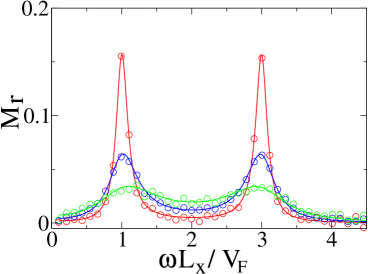
Figure 1: (color online) Dependence of the rescaled magnetization $M_{r}=-2M/M_{0}$ on the rescaled microwave frequency $\omega/\omega_{x}$ for a quantum dot with a harmonic potential at $\omega_{y}/\omega_{x}=3$ (see definitions of $M_{0}$ and $M_{r}$ in Eq (43)). Here $L_{x}=v_{F}/\omega_{x}$ and $v_{F}$ is the velocity Fermi at the Fermi energy $E_{F}$. The rescaled relaxation rate is $\gamma/\omega_{x}=0.1;0.25;0.5$ (red, blue, green curves/circles from top to bottom at $\omega/\omega_{x}=1$). Circles show numerical data obtained from Eq.(30) by integration of classical dynamics and Monte Carlo averaging over $10^{4}$ trajectories from the Fermi-Dirac equilibrium distribution at zero temperature; full curves show the theoretical result given by Eqs.(21)-(25).

To obtain the expression for $L$ we used above the quantum Kubo theory. However, the result (22) has a purely classical form and therefore it is useful to try to obtain it from the classical kinetic theory. With this aim let us consider an arbitrary two dimensional system with a Hamiltonian $H=H(q_{x},p_{x},q_{y},p_{y},t)$. Then the kinetic equation for the distribution function $\rho(\mathbf{x})$ pitaevsky reads

$$\frac{\partial\rho}{\partial t}+\{H,\rho\}=-\gamma(\rho-\rho_{0})$$ (27)

where $\rho_{0}$ is the equilibrium thermal distribution, $\{H,f\}$ are the Poisson brackets and for simplicity of notations $\mathbf{x}=(x,p_{x},y,p_{y})$. After a change of variables $(t^{\prime},\mathbf{x^{\prime}})=(t,T_{0,t}\mathbf{x})$ this equation is reduced to

$$\frac{\partial\rho(\mathbf{x^{\prime}},t^{\prime})}{\partial t^{\prime}}=-\gamma(\rho(\mathbf{x^{\prime}},t^{\prime})-\rho_{0}(T_{t^{\prime},0}\mathbf{x^{\prime}}))$$ (28)

where $T_{t^{\prime},t}$ notes the time evolution operator from time $t$ to time $t^{\prime}$ given by the dynamics of the Hamiltonian $H$. This equation can be solved explicitly that leads to the time averaged distribution function :

$$<\rho(\mathbf{x},t)>_{t}=\gamma\int_{-\infty}^{0}e^{\gamma t^{\prime}}<\rho_{0}(T_{t+t^{\prime},t}\mathbf{x})>_{t}dt^{\prime}$$ (29)

where $T_{t+t^{\prime},t}$ is the time evolution operator in the phase space. Then the average of any quantity $Q(\mathbf{x})$ (for example $Q=xp_{y}-p_{x}y$) can now be expressed as :

$$<Q(\mathbf{x})>=\int Q(\mathbf{x})<\rho(\mathbf{x},t)>_{t}dx=$$

$$\gamma<\int_{-\infty}^{0}e^{\gamma t^{\prime}}(\int Q(\mathbf{x})\rho_{0}(T_{t+t^{\prime},t}\mathbf{x})dx)dt^{\prime}>_{t}=$$

$$\gamma\int dx\rho_{0}(\mathbf{x})\int_{-\infty}^{0}dt^{\prime}e^{\gamma t^{\prime}}<Q(T_{t,t+t^{\prime}}\mathbf{x})>_{t}=$$

$$\gamma\int dx\rho_{0}(\mathbf{x})\int_{0}^{\infty}dt^{\prime}e^{-\gamma t^{\prime}}<Q(T_{t+t^{\prime},t}\mathbf{x})>_{t}\quad.$$ (30)

Here it is used that the transformation $\mathbf{x^{\prime}}=T_{t+t^{\prime},t}\mathbf{x}$ is area-preserving in the phase space. For the case of two oscillators with frequencies $\omega_{x},\omega_{y}$ the time evolution can be find explicitly so that for dynamics in $x$ we have

$$\left(\begin{array}[]{l}x(t+t^{\prime})\\ \frac{p_{x}(t+t^{\prime})}{\omega_{x}}\end{array}\right)=\left(\begin{array}[]{ll}\cos\omega_{x}t^{\prime}&\sin\omega_{x}t^{\prime}\\ -\sin\omega_{x}t^{\prime}&\cos\omega_{x}t^{\prime}\end{array}\right)\times$$ (35)

$$\left(\begin{array}[]{l}x-\frac{f_{x}/m}{\omega_{x}^{2}-\omega^{2}}\cos\omega t\\ \frac{p_{x}}{\omega_{x}}+\frac{f_{x}\omega}{(\omega_{x}^{2}-\omega^{2})\omega_{x}}\sin\omega t\end{array}\right)+$$ (38)

$$\left(\begin{array}[]{l}\frac{f_{x}/m}{\omega_{x}^{2}-\omega^{2}}\cos\omega(t+t^{\prime})\\ -\frac{\omega f_{x}}{(\omega_{x}^{2}-\omega^{2})\omega_{x}}\sin\omega(t+t^{\prime})\end{array}\right)$$ (41)

with a similar equation for $y,p_{y}$. After averaging over $t$ we obtain

$$<x(t+t^{\prime})p_{y}(t+t^{\prime})>_{t}=\frac{\omega}{2}\frac{f_{x}}{(\omega_{x}^{2}-\omega^{2})}\frac{f_{y}/m}{(\omega_{y}^{2}-\omega^{2})}\times$$

$$[-\frac{\omega_{y}}{\omega}\sin(\omega_{y}t^{\prime})\cos(\omega_{x}t^{\prime})+\sin\omega t^{\prime}\cos(\omega_{x}t^{\prime})+$$

$$\frac{\omega}{\omega_{x}}\sin(\omega_{x}t^{\prime})\cos(\omega_{y}t^{\prime})-\frac{\omega}{\omega_{x}}\sin(\omega_{x}t^{\prime})\cos\omega t^{\prime}]$$ (42)

with a similar expression for $<y(t+t^{\prime})p_{x}(t+t^{\prime})>_{t}$. After substitution of (42) in (30) the integration over $t^{\prime}$ gives exactly the expression (22) with $I(\omega)$ given by Eqs.(23)-(25). The integration can be done analytically or with help of Mathematica package. This result shows that the average momentum $L$ can be exactly obtained from the classical formula (30).

A comparison of results of numerical simulations of classical dynamics with Monte Carlo averaging over large number of trajectories from an equilibrium distribution is shown in Fig1. The numerical data clearly confirm the validity of the theoretical expressions given by Eqs.(22)-(25).

It is interesting to note that if instead of Eq.(9) for the density matrix one would assume an adiabatic switching of microwave field with a rate $\gamma$ then the average induced momentum $L$ would be given by the classical relation (4) for a classical oscillator. Indeed, such a procedure simply induces an imaginary shift in driving frequency. Such type of switching had been assumed in chaplik and may be considered to give a qualitatively correct result even if a rigorous description is given by Eq.(9) with the final answer in the form of Eqs.(21-25) being quantitatively different from Eq.(9).

For comparison with the physical values of magnetic moment $M$ in real quantum dots it is convenient to use rescaled momentum $M_{r}$. To do this rescaling we note that the magnetic moment is expressed via the orbital momentum as $M=eL/(2mc)$ (in SGS units). Due to the relation (21) it is convenient to choose a unit of orbital momentum induced by a microwave field for one electron as $L_{0}=mv_{F}L_{x}(f_{x}f_{y}L_{x}^{2})/E_{F}^{2}$ where $E_{F}=mv_{F}^{2}/2$ is the Fermi energy in a dot. Then the unit of magnetic momentum is $M_{0}=eNL_{0}/mc$ where $N$ is the number of electrons in a dot. This implies that the physical magnetic moment $M$ can be expressed via our rescaled value according to the relations

$$M=-M_{r}M_{0}/2,\;M_{0}=eNL_{0}/mc,\;$$

$$M_{0}=eNv_{F}L_{x}(f_{x}f_{y}L_{x}^{2})/(cE_{F}^{2}).$$ (43)

where the oscillation frequency in $x$ is $\omega_{x}=V_{F}/L_{x}$. It is important to stress that the total magnetization of the dot is proportional to the number of electrons in a dot with fixed $E_{F}$.

3 Dots with an enharmonic potential

It is very important to extent the methods developed above to a generic case of enharmonic potential inside a dot. With this aim we consider the case of 2D quartic nonlinear oscillator described by the Hamiltonian

$$H=(p_{x}^{2}+p_{y}^{2})/2m+(r_{x}^{2}x^{4}+r_{y}^{2}y^{4}+2Kx^{2}y^{2})/4.$$ (44)

For $K=0$ we have two decoupled quartic oscillators. Due to nonlinearity the frequencies of oscillations scale with energy as $\omega_{x,y}\approx 1.2(r^{2}_{x,y}E_{F}/m^{2})^{1/4}$ (see e.g. chirikov1979 ). In this case $L_{x}=(4E_{F}/r_{x}^{2})^{1/4}$, $L_{y}=(4E_{F}/r_{y}^{2})^{1/4}$ and we choose the fixed ratio $L_{y}/L_{x}=\sqrt{r_{x}/r_{y}}=1/\sqrt{3}$ for our studies. The rescaled momentum and magnetization are again given by Eq.(43).

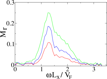
Figure 2: (color online) Dependence of rescaled momentum $M_{r}$ given by Eq.(43) on rescaled frequency $\omega L_{x}/v_{F}$ for the case of quartic oscillator with the Hamiltonian (44) at $K=0$ and $L_{y}/L_{x}=1/\sqrt{3}$ ($r_{x}/r_{y}=1/3$), the monochromatic field has $f_{x}=f_{y}$ and $f_{x}L_{x}/E_{F}=0.25??$. Curves correspond to different values of the relaxation rate $\gamma L_{x}/v_{F}$ = 0.03 (red), 0.06 (blue), 0.14 (green) (from bottom to top at $\omega L_{x}/v_{F}=1.2$). The curves are obtained from Eq.(30) by integration of classical dynamics and Monte Carlo averaging over $10^{4}$ trajectories from the Fermi-Dirac distribution at zero temperature.

The value of averaged orbital momentum is obtained by numerical integration of hamiltonian equations of motion in presence of a linear-polarized monochromatic field (see (1), (44)). The effects of relaxation to stationary state with a rate $\gamma$ are taken into account via relation (30). The average momentum $<L>$ is obtained by Monte Carlo averaging over $10^{4}$ trajectories from the Fermi-Dirac distribution at zero temperature. The integration time is about $10^{4}$ oscillation periods.

The dependence of rescaled magnetization on microwave frequency $\omega$ for different relaxation rates is shown in Figs.2,3. In contrast to the case of harmonic potential the dependence on frequency is characterized by a broad distribution with a broad peak centered approximately near oscillation frequency $\omega_{x}=1.2(r_{x}^{2}E_{F}/m^{2})^{1/4}\approx 1.2v_{F}/L_{x}$. Significant magnetization is visible essentially only inside the interval $\omega_{x}\approx 1.2v_{F}/L_{x}<\omega<\omega_{y}\approx 2.1v_{F}/L_{x}$. Data obtained also show that at small relaxation rates magnetization drops to zero approximately as $M_{r}\propto\gamma$ (see Fig.2). Also $M_{r}$ drops with the increase of $\gamma$ at large $\gamma$ (see Fig.3). This behaviour is qualitatively similar to the case of harmonic potential (see Eqs.(5),(6)).

It is important to note that according to data shown in Fig.4 the coupling between $x,y$-modes, which generally leads to a chaotic dynamics chirikov1979 , does not lead to significant modifications of the magnetization spectrum. Only at rather large values of $K$, when the modes are strongly deformed, the spectrum starts to be modified.

To show that the magnetization dependence on frequency found for the quartic oscillator (44) represents a typical case we also study magnetization in chaotic billiards described in the next Section.

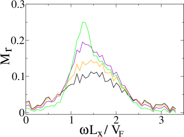
Figure 3: (color online) Same as in Fig.2 but for $\gamma L_{x}/v_{F}$ = 0.14 (green), 0.3 (violet), 0.45 (yellow), 0.55 (black) (from top to bottom at $\omega L_{x}/v_{F}=1.2$).

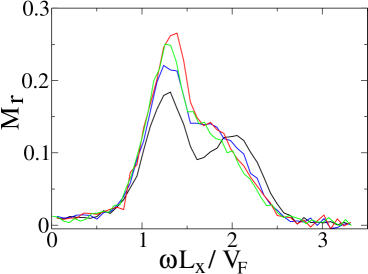
Figure 4: (color online) Same as in Fig.2 for $\gamma L_{x}/v_{F}=0.14$ and different coupling strength $K$ between $x,y$-modes in (44): $KL_{x}^{4}/E_{F}=$ 4 (red), 0 (green), 8 (blue), 16 (black) (from top to bottom at $\omega L_{x}/v_{F}=1.3$).

4 Magnetization in chaotic billiards

To study microwave induced magnetization in billiards we choose the Bunimovich stadium billiard bunimovich as a typical example. The semicircle radius is taken to be $R$, the total size of stadium in $x$ is $L_{x}$, and in $y$ it is $L_{y}=2R$. Usually we use $L_{x}=3.5R$ (see Fig.5). Inside the billiard the particle is affected only by monochromatic force, the collisions with boundaries are elastic.

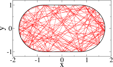
Figure 5: (color online) Example of a trajectory inside the Bunimovich stadium dot in presence of microwave driving. The system parameters are $L_{x}/R=3.5,L_{y}/R=2$, microwave polarization angle $\theta=\pi/4$ ($f_{x}=f_{y}$), $fR/E_{F}=0.28$, $\omega L_{x}/V_{F}=1.7$, $T/E_{F}=0.1$, $v_{F}\tau_{rel}/R\approx 2$, $v_{F}\tau_{i}/R\approx 500$.

To take into account that without monochromatic force the particles relax to the Fermi-Dirac equilibrium we used the generalized Metropolis approach developed in alik . Namely, after a time interval $\Delta t$ the kinetic energy of particle $E$ is changed randomly into the interval $(E-\Delta E,E+\Delta E)$ with a probability given by the Fermi-Dirac distribution at given temperature $T$. The change takes place only in energy while the velocity direction remains unchanged (see below). This procedure imposes a convergence to the Fermi-Dirac equilibrium with the relaxation time $\tau_{rel}\approx\Delta t(E_{F}/\Delta E)^{2}$ (see alik for detailed description of the algorithm). In the numerical simulations we usually used $v_{F}\Delta t/R\approx 0.05$ and $\Delta E/E_{F}=0.15$. At such parameters a particle propagates on a sufficiently large distance during the relaxation time: $v_{F}\tau_{rel}/R\approx 2$. In absence of $ac-$driving the Metropolis algorithm described above gives a convergence to the Fermi-Dirac distribution with a given temperature $T$. In presence of microwave force the algorithm gives convergence to a certain stationary distribution which at small force differs slightly from the Fermi-Dirac distribution (the dependence of deformed curves on energy is similar to those shown in Fig.2 of Ref. alik ). However, in contrast to the unperturbed case, the perturbed stationary distribution has an average nonzero orbital and magnetic momentum $M$. The dependence of average momentum $M$ on temperature $T$ is relatively weak if $T\ll E_{F}$ and therefore, the majority of data are shown for a typical value $T/E_{F}=0.1$ (see more detail below). To take into account the effect of impurities the velocity direction of a particle is changed randomly in the interval $(0,2\pi)$ after a time $\tau_{i}$. Usually we use such $\tau_{i}$ value that the mean free path is much larger than the size of the billiard $v_{F}\tau_{i}/R\approx 500$, in this regime the average momentum is not affected by $\tau_{i}$ (see below). The average momentum is usually computed via one long trajectory which length is up to $10^{7}$ times longer than $R$; computation via 10 shorter trajectories statistically gives the same result. An example of typical trajectory snapshot is shown in Fig.5. It clearly shows a chaotic behaviour (the lines inside the billiard are curved by a microwave field).

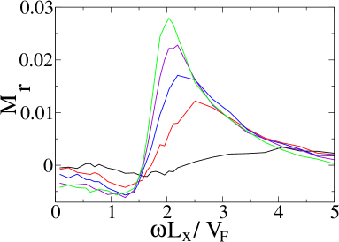
Figure 6: (color online) Rescaled momentum $M_{r}$ as a function of rescaled microwave frequency $\omega L_{x}/v_{F}$ in the Bunimovich billiard. All parameters are as in Fig.5, curves correspond to different values of relaxation time $\tau_{rel}$ with $v_{F}\tau_{rel}/R=$ 0.5 (green), 0.7 (violet), 1.1 (blue), 2 (red), 8 (black) (from top to bottom at $\omega L_{x}/V_{F}=2$).

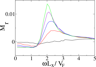
Figure 7: (color online) Same as in Fig.6 but the length of stadium is increased so that here $L_{x}/R=5$.

The numerical data for dependence of average rescaled momentum $M_{r}$ (see Eq. (43)) on rescaled microwave frequency $\omega L_{x}/v_{F}$ are shown in Fig. 6 for polarization $\theta=\pi/4$. Qualitatively, the dependence is similar to the case of nonlinear oscillator discussed in previous Section (see Figs. 2-4). At the same time, there is also a difference in the behaviour at small frequency ($\omega L_{x}/v_{F}<1.5$) where the momentum changes sign. At small relaxation times $\tau_{rel}$ the frequency dependence has a sharp peak near   $\omega L_{x}/v_{F}\approx 2$. The increase of $\tau_{rel}$ leads to a global decrease of average magnetization, that is similar to the data of Fig. 2, also the peak position shifts to a bit higher $\omega$. Let us also note that according to our numerical date the rescaled momentum $M_{r}$ is independent of the strength of driving force $f$ in the regime when $fR/E_{F}<0.5$. This is in the agreement with the relation (43).

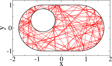
Figure 8: (color online) Example of a trajectory inside a dot in a form of the Bunimovich stadium with a circular “impurity” inside the billiard. The billiard boundary is as in Fig.5, the circular impurity has the radius $r=R/2$, its center is located at $x=-0.75R$, $y=R/3$ counting from the center of the stadium. The system parameters are as in Fig.5 except that the polarization angle $\theta=0$.

The position of peak is determined by the frequency of oscillations along long $x$-axis of the billiard. Indeed, an increase of this size of billiard from $L_{x}=3.5R$ (Fig. 6) to $L_{x}=5R$ (Fig. 7) keeps the shape of resonance curves practically unchanged. At the same time the rescaled magnetization drops approximately by a factor 2. This means that there is no significant increase of $M$ with increase of $L_{x}$ ($M_{0}$ grows by a factor 2.9). From a physical view point, it is rather clear since in the regime with $L_{x}\gg L_{y}$ further increase of $L_{x}$ cannot lead to increase of magnetization. This means that in Eq.(43) the value of $M_{0}$ gives a correct estimate of real magnetization assuming that $L_{x}\sim L_{y}$,

The Bunimovich billiard has varies symmetries, namely $x\rightarrow-x$, $y\rightarrow-y$. It is interesting to study the magnetization properties when all of them are absent. With this aim we introduced an elastic disk scatterer inside the billiard as it is shown in Fig. 8. The dependence of rescaled magnetization $M_{r}$ on rescaled frequency $\omega L_{x}/v_{F}$ is shown for this “impurity” billiard in Fig. 9 for two polarization angles $\theta=\pi/4$ and $\theta=0$. For $\theta=\pi/4$ the behaviour in Fig. 9 is rather similar to the case of billiard without impurity (see Fig. 6), taking into account that $M_{0}$ values differ by a factor two that gives smaller $M_{r}$ values in Fig. 9. In addition the peak at $\omega L_{x}/v_{F}=2$ is more broad that can be attributed to contribution of orbits with a shorter periods colliding with the impurity. The case of polarization with $\theta=0$ is rather different. Indeed, here the average magnetization exists even if in the billiard case $M_{r}=0$ due to symmetry. Also the sign of the momentum (magnetization) is different comparing to the case of $\theta=\pi/4$ polarization. For the impurity billiard we find that at $\theta=0$ the absolute value of magnetization decreases with the increase of relaxation time $\tau_{rel}$ in a way similar to one should in Figs. 6,7.

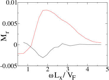
Figure 9: (color online) Dependence of rescaled momentum $M_{r}=-2M/M_{0}$ on rescaled frequency $\omega L_{x}/v_{F}$ for the Bunimovich stadium with impurity shown in Fig.8. Here $fR/E_{F}=0.28$, $\theta=0$ (bottom black curve) and $fR/E_{F}=0.2$, $\theta=\pi/4$ (top red/gray curve); also in this Figure we use definition $M_{0}=eNv_{F}L_{x}(f^{2}L_{x}^{2})/(cE_{F}^{2})$ which is more suitable for polarization with $\theta=0$. Other parameters are $T/E_{F}=0.1$, $v_{F}\tau_{rel}/R\approx 2$, $v_{F}\tau_{i}/R\approx 500$ (cf. with corresponding case in Fig. 6).

The polarization dependence of magnetization is shown in more detail in Fig. 10 for the Bunimovich stadium (Fig. 5) and the impurity billiard (Fig. 8). In the first case we have $M(\theta)\propto\sin 2\theta$ as in the case of oscillator so that the magnetization averaged over all polarization angles is equal to zero. In contrast to that in the second case when all symmetries are destroyed the averaging over all polarization angles gives nonzero magnetization of the dot. In addition to that internal impurity gives a phase shift in the polarization dependence. The phase shift is due to absence of any symmetry. In such a case we have a more general dependence $M\propto(f_{x}f_{y}+af_{x}^{2}+bf_{y}^{2})$, where $a,b$ are some constants.

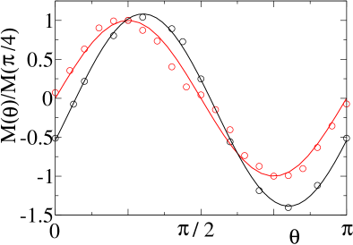
Figure 10: (color online) Dependence of momentum $M$ on polarization angle $\theta$ ($M$ is rescaled to its value at $\theta=\pi/4$) for the Bunimovich stadium (red/gray) and the stadium with circular impurity (black). Numerical data are shown by open circles obtained for $\omega L_{x}/v_{F}=0.78$ (red/gray) and $\omega L_{x}/v_{F}=1.56$ (black) at $fR/E_{F}=0.28$, $T/E_{F}=0.1$, $v_{F}\tau_{rel}/R\approx 2$, $v_{F}\tau_{i}/R\approx 500$. Smooth red/gray curve shows the theoretical dependence $\sin 2\theta$; black curve shows a numerical fit $M(\theta)/M(\pi/4)=-0.15+1.23\sin(2\theta-0.32)$.

In addition, we also checked that if at $\theta=0$ the disk impurity inside the billiard is replaced by a semidisk of the same radius then the dependence on the parameters remains essentially the same, as well as the sign of magnetization (the disk is divided by a vertical line onto two semidisks and left semidisk is removed). It is interesting to note that a negative sign of $M_{r}$ means anti-clockwise rotation. This direction of current rotation can be also understood in a link with ratchet flow on the semidisk Galton board studied in ratchet1 ; ratchet2 ; alik . The link with the ratchet effect becomes especially clear if to consider the semidisk ratchet billiard shown in Fig. 11. Here, due to the ratchet effect discussed in ratchet1 ; ratchet2 ; alik for polarization $\theta=0$ electrons should move to the left in the upper half of the billiard and to the right in the bottom half, thus creating negative magnetization $M_{r}$. We think that if only upper semidisk is left still the direction of rotation at $\theta=0$ microwave polarization is due to the particle flow directed from right to left in the upper part of the billiard that corresponds to negative sign of magnetization $M_{r}$ in Fig. 9.

Figure 11: Example of a billiard with ratchet effect. Collisions with the stadium and internal boundaries are elastic.

Finally, let us make few notes about the dependence of magnetization $M_{r}$ on the impurity scattering time $\tau_{i}$ and temperature $T$. For example, for the impurity billiard of Fig. 8 at $\theta=0$ we find that the variation of $M_{r}$ is about $10\%$ when $v_{F}\tau_{i}/R$ is decreased from $500$ down to $50$, and then $M_{r}$ drops approximately linearly with $v_{F}\tau_{i}/R$ (e.g. $M_{r}(v_{F}\tau_{i}/R=10)/M_{r}(v_{F}\tau_{i}/R=50)=0.47$, $M_{r}(v_{F}\tau_{i}/R=5)/M_{r}(v_{F}\tau_{i}/R=50)=0.2$, $M_{r}(v_{F}\tau_{i}/R=2.5)/M_{r}(v_{F}\tau_{i}/R=50)=0.08$. The decrease of magnetization with decrease of $\tau_{i}$ is rather natural since the ballistic propagation of a particle between boundaries disappears as soon as the scattering mean free path $v_{F}\tau_{i}$ becomes smaller than the billiard size $L_{x}$. Similar effect has been seen also for the ratchet flow on the semidisk Galton board (see Fig. 9 in Ref.alik ). As far as for dependence on temperature our data show that it was relatively weak in the regime $T/E_{F}\ll 1$. For example, for the set of parameters of Fig. 9 at $\theta=0$ the value of $M_{r}$ is increased only by $14\%$ when $T$ is decreased by a factor 4 (from $T/E_{F}=0.1$ to $T/E_{F}=0.025$) and it is decrease by $40\%$ when $T$ increased from $T/E_{F}=0.1$ to $T/E_{F}=0.2$. This dependence on $T$ shows that the magnetization of the dot remains finite even at zero temperature. This behaviour also has close similarity with the temperature dependence for the ratchet flow discussed in alik ; entin . Such ballistic dots may find possible applications for detection of high frequency microwave radiation at room temperatures. Indeed, the ratchet effect in asymmetric nanostructures, which has certain links with the magnetization discussed here, has been observed at 50GHz at room temperature asong .

5 Discussion

According to the obtained numerical results (see e.g Fig.2) and Eq.(43) the rescaled magnetization of a dot can be as large as $M_{r}/2\sim 0.1$ when the relaxation time $\tau_{rel}$ is comparable with a typical time of electron oscillations in a dot. Thus, the magnetization of a dot is $M=0.1M_{0}$. According to Eq.(43), at fixed electron density the magnetization is proportional to the number of electrons $N$ inside the dot. Due to this the magnetization induced by a microwave field can be much larger than the magnetization induced by persistent currents discussed in levy1990 ; imry ; gilles ; kravtsov1993 ; kravtsov2005 . For example, for 2DES in AlGaAs/GaAs the effective electron mass $m=0.067m_{e}$ and at electron density $n_{e}\approx 2\times 10^{11}cm^{-2}$ we have $E_{F}\approx 100K$, $v_{F}/c\approx 1.4\times 10^{-3}$. Hence, according to Eq. (43) for a microwave field of $f/e=1V/cm$ acting on an electron in a dot of size $L_{x}=1\mu m$ we obtain $N\approx 2\times 10^{3}$, $fR/E_{F}\approx 0.01$ and $M_{0}/\mu_{B}\approx 2m_{e}v_{F}L_{x}N(fL_{x}/E_{F})^{2}/\hbar\approx 5\times 10^{3}N(fL_{x}/E_{F})^{2}\approx 10^{3}$, where $\mu_{B}=e\hbar/(2m_{e}c)$ is the Bohr magneton. Nowadays technology allows to produce samples with very high mobility so that the mean free path can have values as large as few tens of microns at $4K$. At $n_{e}=const$ we have the scaling $M_{0}\propto L_{x}^{5}f^{2}$ and for an increased dot size $L_{x}=10\mu m$ and field $f/e=3V/cm$ the magnetization of one dot is $M\approx 0.1M_{0}\approx 10^{8}\mu_{B}$ being comparable with the total magnetization of $10^{7}$ rings in levy1990 . Therefore, this one dot magnetization induced by a microwave field can be observed with nowadays experimental possibilities bouchiat1 ; bouchiat2 ; heitman . We note that the magnetization is only weakly dependent on temperature but the mean free pass at given temperature should be larger than the dot size.

This ballistic magnetization should also exist at very high frequency driving, e.g. THz or optical frequency, which is much larger than the oscillation frequency. In this regime the magnetization drops with the driving frequency $M\propto 1/\omega^{2}$ (see Eqs. (21)-(25)) but this drop may be compensated by using strong driving fields.

From the theoretical view point many questions remain open and further studies are needed to answer them. Thus, an analytical theory is needed to compute the magnetization in dots with enharmonic potential or billiards. On a first glance, as a first approximation one could take analytical formulas for harmonic dot Eqs. (21)-(25) and average this result over frequencies variation in an enharmonic dot. However, in the limit of small relaxation rate $\gamma$ (or large $\tau_{rel}$) such an averaging gives finite magnetization independent of $\gamma$. Indeed, in analogy with the Landau damping landau ; pitaevsky such integration gives effective dissipation independent of initial $\gamma\rightarrow 0$. Appearance of such magnetization independent of $\gamma$ would be also in a qualitative agreement with the results obtained for ratchet transport on the semidisk Galton board ratchet2 ; alik and in the asymmetric scatterer model studied in entin . Indeed, according to these studies the velocity of ratchet is independent of the relaxation rate in energy (relaxation over momentum direction is reached due to dynamical chaos). In fact this indicates certain similarities with the Landau damping where the final relaxation rate is independent of the initial one. Also, the results obtained in alik ; entin show that the ratchet velocity can be obtained as a result of scattering on one asymmetric scatterer. Therefore, it is rather tentative to use the semidisk billiard of Fig. 11 and to say that the magnetization in it appears as the result of ratchet flow: for polarization $\theta=0$ the ratchet flow goes on the left in the upper part of the billiard and on the right in the bottom part. The velocity of such ratchet flow $v_{f}$ in this 2DES is given by the relations found in alik ; entin , namely $v_{f}/v_{F}\sim(fR/E_{F})^{2}$. This flow gives a magnetization of billiard dot induced by a microwave field which is of the same order as $M_{0}$ in the relation (43). However, in this approach the rescaled momentum $M_{r}$ is simply some constant independent of the relaxation rate in energy, as it is the case for the ratchet transport on infinite semidisk lattice. This result is in the contradiction with our numerical data for magnetization dependence on the relaxation rate in energy which gives approximately $M_{r}\propto\gamma L_{x}/v_{F}\sim L_{x}/(v_{F}\tau_{rel})$ (see Figs.2,6,7). A possible origin of this difference can be attributed to the fact that the ratchet flow is considered on an infinite lattice while the magnetization takes place in a confined system and the relaxation properties are different in these two cases.

Also we should note that here we used approximation of noninteracting electrons and neglected all collective effects. In principle, it is well known that microwave radiation can excite plasmons in 2DES (see e.g, weiss ). These excitations can be viewed as some oscillatory modes with different frequencies $\omega_{x},\omega_{y}$ and therefore in analogy with Eqs. (21)-(25) it is natural to expect that a liner-polarized radiation can also create rotating plasmons with finite magnetization induced by this rotation. In addition, the effects of screening should be also taken into account. All these notes show that further theoretical studies are needed for a better understanding of radiation induced magnetization in 2DES dots.

We thank Kvon Ze Don for useful discussions and for pointing to us Ref.chaplik at the final stage of this work. This work was supported in part by the ANR PNANO project MICONANO.

References

• (1) L.P. Lévy, G. Dolan, J. Dunsmuir, and H. Bouchiat, Phys. Rev. Lett. 64, 2074 (1990).
• (2) Y. Imry, Introduction to mesoscopic physics, Oxford Univ. Press, Oxford (1997).
• (3) E. Akkermans, and G. Montambaux, Physique mésoscopique des électron et des photons, EDP Sciences, Les Ulis (2004).
• (4) J.E. Mayer, and M. Goeppert-Mayer, Statistical mechanics, John Wiley & Sons, N.Y., (1977).
• (5) D. Mailly, C.Chapelier, and A. Benoit, Phys. Rev. Lett. 70, 2020 (1993).
• (6) V.E. Kravtsov, and V.I. Yudson, Phys. Rev. Lett. 70, 210 (1993).
• (7) V.E. Kravtsov, in Nanophysics: coherence and transport, Lecture Notes of the Les Houches Summer School 2004, Eds. H. Bouchiat, Y.Gefen, S. Guéron, G. Montambaux, and J. Dalibard, Elsevier, Amsterdam (2005) (cond-mat/0504671).
• (8) R. Deblock, R. Bel, B. Reulet, H. Bouchiat, and D. Mailly, Phys. Rev. Lett. 89, 206803 (2002).
• (9) R. Deblock, Y. Noat, B. Reulet, H. Bouchiat, and D. Mailly, Phys. Rev. B 65, 075301 (2002).
• (10) A. Pikovsky, M. Rosenblum and J. Kurths, Synchronization: a universal concept in nonlinear sciences, Cambridge University Press, Cambridge (2001).
• (11) L.I. Magarill, and A.V. Chaplik, JETP Lett. 70, 615 (1999) [Pis’ma Zh. Eksp. Teor. Fiz. 70, 607 (1999)].
• (12) A.D. Chepelianskii, and D.L. Shepelyansky, Phys. Rev. B 71, 052508 (2005).
• (13) G. Cristadoro, and D.L. Shepelyansky, Phys. Rev. E 71, 036111 (2005).
• (14) A.D. Chepelianskii, Eur. Phys. J. B 52, 389 (2006).
• (15) M.V. Entin, and L.I. Magarill, Phys. Rev. B 73, 205206 (2006).
• (16) L.D. Landau, Zh. Eksp. Teor. Fiz. 11, 592 (1941).
• (17) E.M. Lifshitz, and L.P. Pitaevskii, Physical kinetics, Pergamon Press, Oxford (1981).
• (18) L.A. Bunimovich, Billiards and other hyperbolic systems, in Dynamical Systems, Ergodic Theory and Applications, Ed. Y.G.Sinai, Series: Encyclopaedia of Mathematical Sciences Vol. 100, Springer, Berlin (2000).
• (19) B.V.Chirikov, Phys. Rep. 52, 263 (1979).
• (20) M.P. Schwarz, D. Grundler, Ch.Heyn, D. Heitmann, D. Reuter and A. Wieck, Phys. Rev. B 68, 245315 (2003).
• (21) A.M. Song, P. Omling, L. Samuelson, W. Seifert, I.Shorubalko, and H. Zirath, Appl. Phys. Lett. 79, 1357 (2001).
• (22) E. Vasiliadu, R. Fleischmann, D. Weiss, D. Heitmann, K. v.Klitzing, T. Geisel, R. Bergmann, H.Schweizer, and C.T. Foxon, Phys. Rev. B 52, R5658 (1995).