Phase-ordering dynamics in itinerant quantum ferromagnets

Abstract

The phase-ordering dynamics that result from domain coarsening are considered for itinerant quantum ferromagnets. The fluctuation effects that invalidate the Hertz theory of the quantum phase transition also affect the phase ordering. For a quench into the ordered phase there appears a transient regime where the domain growth follows a different power law than in the classical case, and for asymptotically long times the prefactor of the $t^{1/2}$ growth law has an anomalous magnetization dependence. A quench to the quantum critical point results in a growth law that is not a power-law function of time. Both phenomenological scaling arguments and renormalization-group arguments are given to derive these results, and estimates of experimentally relevant length and time scales are presented.

I Introduction

When a many-body system capable of a phase transition from a disordered phase to a phase with long-range order is suddenly taken, by changing one or more parameters, from the disordered phase to the ordered one, an interesting question is how the long-range order will develop as time goes by and the system approaches equilibrium. Such a sudden transformation is called a “quench”, and the phase-ordering dynamics after the quench can be studied by kinetic methods similar to those used for the critical dynamics near the phase transition.Hohenberg and Halperin (1977) The quenching problem is of broad interest since it is applicable to a large variety of physical systems that undergo phase transitions, ranging from magnets to liquid helium to the early universe.Zurek (1985) The phase ordering occurs by means of the growth of domains that arise from spontaneous fluctuations, and the linear size $L$ of these domainsdom obeys a power-law as a function of time $t$ for sufficiently large $t$: $L(t)\propto t^{1/z}$, with $z$ a dynamical exponent.Bray (1994) In addition, the pair correlation function is observed, both experimentally and numerically, to obey a simple scaling law

$$C(r,t)\equiv\langle{\bm{\phi}}({\bm{x}},t)\cdot{\bm{\phi}}({\bm{0}},t)\rangle=f(r/L(t)),$$ (1)

Here $r=|{\bm{x}}|$, $f$ is a scaling function, ${\bm{\phi}}$ is the order parameter field, and $\langle\ldots\rangle$ denotes a statistical average. We take the order parameter to be a real 3-vector, that is, we consider Heisenberg magnets.

The facts stated above, although well established,Bray (1994) are purely phenomenological; so far no derivation from first principles has been given. This phenomenology has so far been applied to classical systems, but there is no reason to expect that it will not be valid for quantum systems as well. Quantum phase transitions are known to differ in crucial aspects from classical ones,Sachdev (1999); Belitz et al. (2005) and one needs to ask whether these differences affect the phase ordering properties as well. In this paper we investigate this problem for the case of a quantum ferromagnet and show that the phase ordering kinetics are indeed affected in dramatic ways.

II Review of results for classical magnets

In order to motivate our approach and put it into context, we first briefly recall the known results for phase ordering in classical magnets. The dynamical equation that governs the time evolution of the order parameter in an isotropic Heisenberg ferromagnet isMa and Mazenko (1975)

$$\frac{\partial{\bm{\phi}}}{\partial t}=\lambda\,{\bm{\nabla}}^{2}\,\frac{\delta H}{\delta{\bm{\phi}}}+\gamma\,{\bm{\phi}}\times\frac{\delta H}{\delta{\bm{\phi}}}+{\bm{\zeta}}.$$ (2)

Here $\lambda$ is a spin transport coefficient, and $\gamma$ is a gyromagnetic ratio. The Langevin force ${\bm{\zeta}}$ is of no consequence for the problem of phase ordering and we will neglect it.Bray (1994) $H$ is the Hamiltonian or free energy functional that governs the equilibrium properties of the system. A classical isotropic Heisenberg ferromagnet is described by a $\phi^{4}$-theory with parameters $r$, $c>0$, and $u>0$Ma (1976)

$$H=\int d{\bm{x}}\,\left[\frac{c}{2}\left(\nabla{\bm{\phi}}\right)^{2}+\frac{r}{2}\,{\bm{\phi}}^{2}+\frac{u}{4}\,({\bm{\phi}}^{2})^{2}\right].$$ (3a)

In Fourier space, this corresponds to a Gaussian vertex

$$\Gamma({\bm{k}})=r+c\,{\bm{k}}^{2}.$$ (3b)

The first term in Eq. (2) describes dissipative dynamics for a conserved order parameter; this is Model B in Ref. Hohenberg and Halperin, 1977. Including the second term takes into account the precession of spins in the effective magnetic field created by all other spins; this is Model J in Ref. Hohenberg and Halperin, 1977.

The phase-ordering problem for Model B ($\gamma=0$) has been studied by a variety of analytic techniques as well as by simulations.Bray (1994) The result is a dynamical exponent $z=4$; i.e., the linear domain size grows for long times as $L(t)\propto t^{1/4}$, with a prefactor that is independent of the equilibrium magnetization $m_{0}$. This result is plausible from a simple power-counting argument: Eq. (2) has the structure of a continuity equation for each component $\phi_{\alpha}$ of the order parameter, $\partial_{t}\,\phi_{\alpha}=-{\bm{\nabla}}\cdot{\bm{j}}_{\alpha}$, and for power counting purposes the current ${\bm{j}}_{\alpha}$ can be identified with the domain growth velocity $dL/dt$ times $m_{0}$. Assuming that each gradient can be identified with a factor of $1/L$,Isi this leads to $dL/dt\sim c\lambda/L^{3}$,not ; gra or

$$L(t)\propto(c\lambda)^{1/4}\,t^{1/4}\quad,\quad\text{(Model B)}.$$ (4)

The additional term in Model J ($\gamma\neq 0$) describes spin waves whose dispersion relation follows from Eq. (2):

$$\omega({\bm{k}})=D(m_{0})\,{\bm{k}}^{2},$$ (5)

with $D(m_{0})=\gamma\,c\,m_{0}\equiv c\Omega_{\text{L}}$, where $\Omega_{\text{L}}=\gamma\,m_{0}$ is the Larmor frequency related to the equilibrium magnetization $m_{0}$. This is consistent with results obtained from microscopic models.Moriya (1985) For the phase ordering problem, Model J was studied in Ref. Das and Rao, 2000. The same power-counting arguments as for Model B above suggest

$$\frac{dL}{dt}\sim\frac{c\lambda}{L^{3}}+\frac{c\,\Omega_{\text{L}}}{L}\ .$$ (6)

According to Eq. (6), the time dependence of $L$ will cross over from the $t^{1/4}$ behavior characteristic for Model B to a $t^{1/2}$ behavior at a length scale $L_{1}=\sqrt{\lambda/\Omega_{\text{L}}}$,

$$L(t)\propto\begin{cases}(c\lambda)^{1/4}\,t^{1/4}&\text{if}\ L\ll L_{1}\cr(c\Omega_{\text{L}})^{1/2}\,t^{1/2}&\text{if}\ L\gg L_{1}\end{cases}\quad,\quad\text{(Model J)}.$$ (7)

A numerical solution of the dynamical equation was found to be in good agreement with this expectation.Das and Rao (2000)

This concludes our review of known results for classical magnets.

III Quantum Ferromagnets

III.1 Mode-mode coupling effects

The above results hold if the equilibrium properties of the ferromagnet are described by Eqs. (3), and if there are no other soft modes that couple to the order parameter. A counterexample is phase separation in binary fluids, where one needs to take into account that the local fluid velocity contributes to the order parameter transport.Bray (1994) The net result is equivalent to a nonlocal free energy, or dynamic equation, and this is obtained explicitly if the additional soft modes are integrated out. At low temperature ($T$) in itinerant ferromagnets a similar phenomenon occurs; viz., a coupling of the order parameter to soft particle-hole excitations.Kirkpatrick and Belitz (1996); Belitz et al. (2001a) These mode-mode coupling effects invalidate Hertz’s mean-field theory,Hertz (1976) and they change both the critical behavior at the ferromagnetic quantum phase transition,Belitz et al. (2001b) and the magnetization dependence of the magnon dispersion relation in the ordered phase.Belitz et al. (1998) Here we investigate how these effects influence the phase ordering following a quench into the quantum regime, which can be realized by a pressure quench at fixed low temperature in a system where the ferromagnetic quantum phase transition can be tuned by hydrostatic pressure, see Fig. 1.

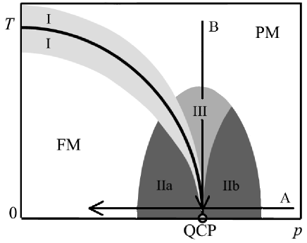
Figure 1: Schematic phase diagram in a temperature (T) - pressure (p) plane with a phase separation line separating a paramagnetic (PM) phase from a ferromagnetic (FM) one. Shown are the quantum critical point (QCP), the classical critical regime (I), and static (IIa,b) and dynamic (III) quantum critical regimes. The arrows denote a quench into the ordered phase (A), and a critical quench (B), respectively. See the text for further explanation, and Ref. Belitz et al., 2005 for a general discussion of magnetic quantum criticality.

Examples of such systems include UGe₂ Saxena et al. (2000) and MnSi.Pfleiderer et al. (1997) The equilibrium quantum phase transitions in these systems have been studied experimentally in some detail, and our predictions for the phase ordering should be amenable to experimental checks using similar methods.

The nature of the mode-mode coupling effects depends on whether the system is dirty or clean, i.e., whether or not quenched disorder is present. In the clean case, they lead to a fluctuation-induced first-order transition,Belitz et al. (1999) so the magnetization cannot be made arbitrarily small. In the dirty case, the quantum phase transition generically is of second order. We will focus on the latter,dis where the size of the quantum effects we consider is not limited by a nonzero minimum value of the magnetization. Quenched disorder also ensures that the transport coefficient $\lambda$ will remain finite even at $T=0$. The form of the dynamical equation (2) will thus not be modified by quantum mechanics. We will briefly discuss clean systems later.

Effectively, the mode-mode coupling effects in a dirty system in $2<d<4$ dimensions lead to a non-local free-energy functional that contains a $\nabla^{d-2}$ term in addition to the usual $\nabla^{2}$ term, or to a Gaussian vertexKirkpatrick and Belitz (1996); Belitz et al. (2005)

$$\Gamma({\bm{k}})=r+{\tilde{c}}\,|{\bm{k}}|^{d-2}+c\,{\bm{k}}^{2}$$ (8)

instead of Eq. (3b), with ${\tilde{c}}>0$. In the ordered phase, this nonanalyticity is cut off by the magnetization, with $m_{0}\sim{\bm{k}}^{2}$. It is also cut off by $T>0$. We will discuss the latter effect, as well as the behavior at criticality, below; for now we assume any length scale associated with temperature to be the largest scale in the system, which effectively sets $T=0$, and a quench well into the ordered phase, see trajectory A in Fig. 1.tra Let us denote the length scale where $m_{0}$ cuts off the nonanalyticity by $L_{2}(m_{0})\propto m_{0}^{-1/2}$, and the length scale beyond which the nonanalyticity dominates by $L^{*}=(c/{\tilde{c}})^{1/(4-d)}$. (We will determine and discuss $L_{2}$ and $L^{*}$ in more detail below.) Since the dissipative term and the torque term in Eq. (2) are both proportional to $\delta H/\delta{\bm{\phi}}$, they are equally affected. Equation (8) implies that, effectively, $\delta H/\delta{\bm{\phi}}=-c\nabla^{2}{\bm{\phi}}$ which would result from Eq. (3a) gets multiplied by a function $f(\nabla,m_{0})$, where $\nabla$ stands for the appropriate inverse length scale, which is $|{\bm{k}}|$ for the magnon dispersion, and $1/L$ for the phase ordering problem. For scales larger than $L^{*}$, we have

$$f(\nabla,m_{0})\propto\begin{cases}(L^{*}\,\nabla)^{d-4}\propto\nabla^{d-4}&\text{if}\ 1/\nabla\ll L_{2}\cr(L^{*}/L_{2})^{d-4}\propto m_{0}^{-(4-d)/2}&\text{if}\ 1/\nabla\gg L_{2}\ .\end{cases}$$ (9)

For an illustration of these effects, let us consider the magnon dispersion relation. The above considerations result in Eq. (5) with a modified $D(m_{0})$, viz., $D(m_{0})\propto m_{0}^{(d-2)/2}$, for $|{\bm{k}}|\ll 1/L_{2}$, and in $\omega({\bm{k}})\propto|{\bm{k}}|^{d-2}$ for $|{\bm{k}}|\gg 1/L_{2}$. The former result was first obtained in Ref. Belitz et al., 1998 from microscopic considerations, and we have reproduced it here as an illustrative check on our power-counting technique.

III.2 The quantum phase ordering problem

For the phase ordering problem, the right-hand side of Eq. (6) gets multiplied by $f(1/L,m_{0})$,

$$\frac{dL}{dt}\sim\left(\frac{c\lambda}{L^{3}}+\frac{c\,\Omega_{\text{L}}}{L}\right)\,f(1/L,m_{0}).$$ (10)

In $d=3$, the domain growth then displays four different power laws in different time or length regimes, as follows:

$$L(t)\propto\begin{cases}(c\lambda/L^{*})^{1/3}\,t^{1/3}&\text{if}\ L<\{L_{1},L_{2}\}\cr(c\Omega_{\text{L}}/L^{*})\,t&\text{if}\ L_{1}<L<L_{2}\cr(c\lambda L_{2}/L^{*})^{1/4}\,t^{1/4}\cr\hskip 20.0pt\propto m_{0}^{-1/8}\,t^{1/4}&\text{if}\ L_{2}<L<L_{1}\cr(c\Omega_{\text{L}}L_{2}/L^{*})^{1/2}\,t^{1/2}\cr\hskip 35.0pt\propto m_{0}^{1/4}t^{1/2}&\text{if}\ \{L_{1},L_{2}\}<L\ .\end{cases}$$ (11)

Compared to Eq. (7), the asymptotic time dependence of $L$ remains unchanged, but the dependence of the prefactor on the equilibrium magnetization is $m_{0}^{1/4}$ instead of $m_{0}^{1/2}$. In the initial scaling regime, where $L<L_{1}$, the time dependence is $t^{1/3}$ instead of $t^{1/4}$ in the classical case. In addition, there is an intermediate regime where $L(t)$ grows as $t$ if $L_{1}<L_{2}$, and as $t^{1/4}$ if $L_{2}<L_{1}$.

Equation (11) is the central new result of the present paper. It has been derived entirely by power counting, that is, from Eq. (10) which associated all gradients in the problem with powers of $1/L$. Next we establish the validity of this procedure by means of a renormalization-group analysis that generalizes Bray’s analysis of Model B.Bray (1990)

III.3 Renormalization-group considerations

Adapting the renormalization procedure of Ma,Ma (1976) we assign a scale dimension $[L]=-1$ to $L$, and a scale dimension $[t]=-z$ to time. Equation (1) suggests to choose the field ${\bm{\phi}}({\bm{x}},t)$ to be dimensionless, $[{\bm{\phi}}({\bm{x}},t)]=0$. Let the Fourier transform of $C$ in Eq. (1) be $S({\bm{k}},t)=\int d{\bm{x}}\,\exp(-i{\bm{k}}\cdot{\bm{x}})\,C(r,t)$. The exponent $\eta$ is defined by the structure factor $S({\bm{k}})=S({\bm{k}},t\to\infty)$ to behave as $S({\bm{k}})\propto|{\bm{k}}|^{-2+\eta}$; this implies $\eta=2-d$. Position, time, and fields are then rescaled in the RG process according to ${\bm{x}}^{\prime}={\bm{x}}/b$, $t^{\prime}=t/b^{z}$, and ${\bm{\phi}}^{\prime}({\bm{x}}^{\prime},t^{\prime})={\bm{\phi}}({\bm{x}},t)$, respectively, with $b$ the RG length rescaling factor. The free energy $H$, which has a naive scale dimension equal to zero, is assigned an anomalous scale dimension $-y$, $H^{\prime}[{\bm{\phi}}^{\prime}]=b^{-y}H[{\bm{\phi}}]$. Finally, one needs to keep in mind that the functional derivative of $H$ in Eq. (2) removes a spatial integral and therefore acts, for scaling purposes, like an inverse volume with a scale dimension of $d$. A zero-loop renormalization of Eq. (2) then yields

$$\frac{\partial{\bm{\phi}}^{\prime}}{\partial t^{\prime}}=\lambda^{\prime}\,\nabla^{\prime\,2}\,\frac{\delta H^{\prime}}{\delta{\bm{\phi}}^{\prime}}+\gamma{\,{}^{\prime}}\,{\bm{\phi}}^{\prime}\times\frac{\delta H^{\prime}}{\delta{\bm{\phi}}^{\prime}}.$$ (12a)

with renormalized quantities

$$\lambda^{\prime} = \lambda\,b^{z-d-2+y},$$

$$\gamma{\,{}^{\prime}} = \gamma\,b^{z-d+y}.$$ (12b)

For Model B ($\gamma=0$), the assumption that the transport coefficient $\lambda$ is not singularly renormalized at the fixed point we are looking for (which assumes that a hydrodynamic description remains valid in the ordered phase), leads to the relation $z=d+2-y$,Bray (1990) which expresses the dynamical exponent $z$ in terms of the energy exponent $y$. For Model J this fixed point is not stable: $\gamma$ is relevant with respect to it. Assuming that $\gamma$ is not singularly renormalized (which assumes that the spin waves in the ordered phase are characterized by $\omega({\bm{k}})\propto{\bm{k}}^{2}$), leads to

$$z=d-y.$$ (13)

The remaining question is the value of the anomalous energy dimension $y$. If defects in the order parameter texture determine the scaling properties of the energy, then $y=d-2$ for a vector order parameter.Bray (1990) This yields $z=2$, in agreement with the long-time behavior of $L(t)$. For Model B, the same value of $y$ yields $z=4$.Bray (1990) With increasing length scale, one thus expects a crossover from $z=4$ to $z=2$, as is reflected in Eq. (11). If $L<L_{2}$, then one effectively has $\nabla^{d-2}$ in the free energy instead of $\nabla^{2}$, so one expects $y=d-(d-2)=2$. This leads to $z=d$ for Model B, and $z=d-2$ for Model J, as reflected in the first two lines in Eq. (11). The above considerations show that the naive power-counting considerations that lead to Eq. (6) or (10), which replace all gradients in the dynamical equation by $1/L$, are indeed correct, subject to the above assumptions. Note that for an Ising order parameter, $y=d-1$,Bray (1990) and hence $z=3$ for Model B, so the naive power counting breaks down.Isi

IV Discussion and Conclusion

In the remainder of the paper we provide a semi-quantitative discussion of Eq. (11) by identifying the various length scales that enter the quantum phase ordering problem. $L_{1}$ has been identified in the context of Eq. (7). $L_{2}$ can be identified from the explicit treatment of the ferromagnetic phase in Ref. Sessions and Belitz, 2003. We find $L_{2}=\sqrt{D/\Delta}$, where $D$ is the charge diffusion constant and $\Delta$ is the Stoner gap or exchange splitting. A related scale is $L_{T}=\sqrt{D/T}$, which denotes the length scale where a nonzero temperature cuts off the nonanalyticity. Finally, $L^{*}$ was introduced in connection with Eq. (9). Reference Belitz et al., 2001a yields explicit expressions for the coefficients $c$ and ${\tilde{c}}$, which give $L^{*}=\pi\ell/72$, with $\ell$ the elastic electronic mean-free path due to the quenched disorder. Thus,

$$L_{1} = \sqrt{\lambda/\Omega_{\text{L}}}\quad,\quad L_{2}=\sqrt{D/\Delta}\ ,$$

$$L_{T} = \sqrt{D/T}\hskip 13.0pt,\quad L^{*}=\pi\ell/72\ .$$ (14)

We now estimate the values of these scales. $\Omega_{\text{L}}$ is on the order of $em_{0}/2m_{\text{e}}c$, with $e$ and $m_{\text{e}}$ the electron charge and mass, respectively, and $c$ the speed of light (not to be confused with the coefficient of the square gradient term in the Hamiltonian that is denoted by $c$ everywhere else in this paper). The effects we are considering are largest if the magnetization is small; either because the system is a weak magnet, or because the quench is to just within the ordered phase (but outside the critical region; we consider a critical quench below). For a magnetization $m_{0}=10-100\,{\text{G}}$ we have $\hbar\Omega_{\text{L}}/k_{\text{B}}\approx 0.001-0.01\,\text{K}$. For the Stoner gap one expects $\hbar\Delta/k_{\text{B}}\gtrsim T_{\text{c}}$, with $T_{\text{c}}$ the critical temperature that corresponds to the parameter values after the quench. For low-$T_{\text{c}}$ magnets like MnSi or UGe₂, this means $\hbar\Delta/k_{\text{B}}\approx 10^{2}\,{\text{K}}$. With free-electron parameters, and a Fermi wave number $k_{\text{F}}\approx 1\,\AA^{-1}$, the mean-free path is related to the resistivity $\rho$ by $\ell\approx 10^{3}(\mu\Omega\text{cm}/\rho)\,\AA$, and in the ordered phase one expects $\lambda\approx D\approx\hbar k_{\text{F}}\ell/3m_{\text{e}}$. For $\rho=10\,\mu\Omega\text{cm}$ and $T=1\,{\text{K}}$, a rough estimate for the hierarchy of length scales thus is

$$L^{*} \approx 5\,\AA\hskip 19.0pt,\quad L_{2}\approx 10^{2}\,\AA\ ,$$

$$L_{T} \approx 10^{3}\,\AA\quad,\quad L_{1}\approx 10^{5}\,\AA\ .$$ (15)

For $L^{*}<L<L_{2}$ one has the initial $t^{1/3}$ behavior in Eq. (11). For $L_{2}<L<L_{1}$, the domain size will grow as $L(t)\propto m_{0}^{-1/8}\,t^{1/4}$, and for $L>L_{1}$ the behavior crosses over to $L(t)\propto m_{0}^{1/4}\,t^{1/2}$. With respect to the latter, one should keep in mind that domains larger than a few tens of microns are hard to achieve in zero magnetic field, except close to the critical point.Landau and Lifshitz (1984) These predictions should be observable by time-resolved neutron scattering. In particular, the magnetization dependence of the prefactor of the asymptotic $t^{1/2}$ law can be checked by quenching along trajectory A in Fig. 1 to different final pressure values. By recalling that the parameter $c$ in Eq. (3a) represents the square of a microscopic length scale that is on the order of an $\AA$ we can estimate the time required for a domain to grow to sizes corresponding to the various length scales given in Eq. (15):

$$t^{*} \approx 10^{-15}\,{\rm s}\hskip 6.0pt,\quad t_{2}\approx 10^{-11}\,{\rm s}\ ,$$

$$t_{T} \approx 10^{-7}\,{\rm s}\quad,\quad t_{1}\approx 1\,{\rm s}\ .$$ (16)

Notice that the microscopic time scale for the problem is given by the Fermi wave length divided by the Fermi velocity, which is about $10^{-15}\,{\rm s}$ with free-electron parameters. This is consistent with the value of $t^{*}$.

Now consider a quench into the critical region, which is divided into regimes denoted by I, II, and III in Fig. (1). The classical critical fixed point controls Region I, where phase ordering has been discussed by Das and Rao.Das and Rao (2000) Regions II and III are controlled by the quantum critical fixed point, and the quantum critical behavior is known exactly.Belitz et al. (2001b) Consider a quench to the quantum critical point, trajectory B in the figure.tra The quantum ferromagnetic critical behavior is characterized by logarithmic corrections to scaling, which can be expressed in terms of scale dependent critical exponents. The dynamical critical exponent in $d=3$ is Belitz et al. (2001b, 2005)

$$z=3+\text{const.}\times(\ln\ln b)^{2}/\ln b,$$ (17)

to leading logarithmic accuracy. At the quantum critical point, and in the context of domain growth, the renormalization-group scale factor $b$ represents $1/L(t)$. This leads to a growth law, with the time $t$ measured in arbitrary units,

$$L(t\to\infty)\propto t^{1/3}\,e^{\text{const.}\times(\ln\ln t)^{2}}.$$ (18)

If the quench ends at a low temperature in the critical region, but not at the quantum critical point, $L(t)$ will grow according to Eq. (18) until it becomes comparable to the correlation length $\xi$. In region IIb, at longer times it will saturate at a value comparable to $\xi$, while in region IIa there will be a crossover to the asymptotic behavior as described by Eq. (11). A more complete description of critical quenches will be given elsewhere.us_

In clean systems, analogous mode-mode coupling effects lead to a weaker nonanalytic term than in Eq. (8); in $d=3$ it is ${\bm{k}}^{2}\ln|{\bm{k}}|$. However, the term is negative, which leads to a first-order transition.Belitz et al. (1999) The order of the transition is of no consequence for the phase ordering kinetics, but the requirement of a positive transverse magnetic susceptibility in the ordered phase prevents the magnetization from ever being small enough for the nonanalytic term to dominate over the analytic one. For the magnon dispersion relation, one finds $D(m_{0})=\gamma\,c\,m_{0}[1-\text{const.}\times\ln(1/m_{0})]$, and the equation of state will ensure that $D(m_{0})>0$.mag Similarly, for the phase ordering problem one has $L(t)\propto[1-\text{const.}\times\ln t]\,t^{1/3}$ in a transient regime, and $L(t\to\infty)\propto m_{0}^{1/2}\,[1-\text{const.}\times\ln(1/m_{0})]\,t^{1/2}$ asymptotically (const.$\,>0$). The former result follows since, in the clean limit at $T=0$, $\lambda({\bm{k}}\to 0)\propto 1/|{\bm{k}}|$.

We conclude by summarizing the original results obtained in this paper. First, we generalized the phenomenology that was developed to describe phase ordering following a quench across classical phase transitions to the quantum phase transition case. Second, for the continuous quantum phase transition expected in disordered Heisenberg quantum ferromagnets we obtained the growth laws in various time windows for quenches both deep into the ordered phase and to a point at or very near quantum criticality. Third, we gave the domain growth laws for clean itinerant Heisenberg quantum magnets, where the quantum phase transition is expected to be discontinuous. In the latter case the quantum effects are subleading due to the lower bound on the magnetization imposed by the first-order nature of the transition. All of these results are amenable to experimental verification.