Theory of the Quantum Critical Fluctuations in Cuprates

Abstract

The statistical mechanics of the time-reversal and inversion symmetry breaking order parameter, possibly observed in the pseudogap region of the phase diagram of the Cuprates, can be represented by the Ashkin-Teller model. We add kinetic energy and dissipation to the model for a quantum generalization and show that the correlations are determined by two sets of charges, one interacting locally in time and logarithmically in space and the other locally in space and logarithmically in time. The quantum critical fluctuations are derived and shown to be of the form postulated in 1989 to give the marginal fermi-liquid properties. The model solved and the methods devised are likely to be of interest also to other quantum phase transitions.

A mean-field solution of a microscopic model predicts that the pseudogapped region norman of the phase diagram of the cuprates (Region II in fig.(1) of Ref. (2)) has a spontaneous current pattern depicted in fig.(1a) cmv . Such a state breaks time-reversal, inversion and three of the four reflection symmetries of the square lattice while preserving translational symmetry. The observed magnetic diffraction in neutron scatteringFAQ as well as the dichroism observed in ARPES AK with circularly polarized photons is consistent with such a state.

The transition temperature of this state varies continuously with hole density $x$ and tends to $0$ at $x=x_{c}$, the quantum critical point. Anomalous normal state properties are observed in the funnel shaped region (Region I in fig.(1) of Ref. (2)) emanating from the QCP. They were shown to follow from a phenomenological spectrum mfl :

$$\text{Im}\chi({\bf q},\omega,T) \propto \omega/T,~{}for~{}\omega\ll T,$$

$$\propto constant,~{}for~{}T\ll\omega\ll\omega_{c},$$

where $\omega_{c}$ is a cut-off, determinable from experiments. The corresponding real part of the fluctuations, $Re\chi({\bf q},\omega,T)\propto\ln(\omega_{c}/\omega)$ for $\omega/T\gg 1$ and $\propto\ln(\omega_{c}/T)$ for $\omega/T\ll 1$. Since this spectrum has a singularity in the limit $(T,\omega)\to 0$, it specifies the fluctuations near a quantum critical point. For small ${\bf q}$, this spectrum is directly observed in Raman scattering. raman . The two unusual properties of Eq.Theory of the Quantum Critical Fluctuations in Cuprates, $\omega/T$ scaling sachdev and no dependence (or a smooth dependence) on ${\bf q}$ are sufficient to generate a marginal fermi-liquid mfl . The observed anomalous properties are well explained by the marginal fermi-liquid and its predictions for the single-particle spectra have been verifed in experiments.

The purpose of this work is to show that the quantum critical spectrum of Eq.(Theory of the Quantum Critical Fluctuations in Cuprates) is the spectrum of fluctuations of the order parameter which condense to give the observed order depicted in fig.(1a).

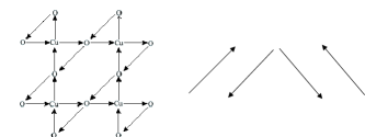
Figure 1: Current pattern(a) and its abstraction (b)

To do so we consider a quantum generalization of the classical model whose solution gives such an order parameter. The four possible configurations in each unit-cell of fig.(1a) can be represented by four vectors with arrows representing time-reversal and orientation representing the only plane of reflection symmetry, as shown in fig.(1b). A classical model with such a pair of Ising degrees of freedom is the Ashkin-Teller BAX model:

$$H=-\sum_{<i,j>}J_{2}(\sigma_{i}\sigma_{j}+\tau_{i}\tau_{j})+J_{4}(\sigma_{i}\tau_{i}\sigma_{j}\tau_{j})$$ (2)

$\sigma_{i}$ and $\tau_{i}$ are Ising spins. Such a Hamiltonian can also be derived cmv from the microscopic model which in mean-field theory gives the observed order parameter provided one neglects amplitude fluctuations.

The Ashkin-Teller model has a variety of phases depending on $J_{4}/J_{2}$ and $T/J_{2}$ BAX ; KD ; MML . Especially interesting to us is the region $-1<J_{4}/J_{2}<0$ in which the ordered phase has ferromagnetic order in $<\sigma_{i}>,<\tau_{i}>$ as well as $<\sigma_{i}\tau_{i}>$ just as in the order observed. Two more properties of this region are of special interest: on the critical line, the model is Gaussian (with stiffness depending on $J_{4}/J_{2}$) and the specific heat at the transition has no divergence.

With the transformation

$$\cos(\theta_{i})=(\sigma_{i}+\tau_{i})/2;~{}\sin(\theta_{i})=(\sigma_{i}-\tau_{i})/2,$$ (3)

the Ashkin-Teller model becomes

$$H=\sum_{i,jnn}2J_{2}\cos(\theta_{i}-\theta_{j})+J_{4}\cos 2(\theta_{i}-\theta_{j})+h_{4}\cos 4\theta_{i}.$$ (4)

The restriction that $\theta_{i}=0,\pi/2,\pi,3\pi/2$ has been written in terms of a four-fold anisotropy term $\propto h_{4}$. Monte-Carlo calculations show sudbo that the classical phase diagram of model (2) and of (3) are the same. This is consistent with the fact that $h_{4}$ is irrelevant above the critical point in the $xy$ model; $h_{4}$ however is relevant below the transition enforcing an Ising state JOS .

For a quantum theory for the model, two additional features are included, the kinetic energy and the dissipation. For the latter, we consider physics of the Caldeira-Leggett type CL , which can be derived by integrating over the fermions in the microscopic model which couples the orbital-currents of $(\theta_{i}-\theta_{j})$ to the currents of the fermions footnoteDISS . For simplicity of presentation, we start with $J_{4}=0$. We will show that no essential modification arises at least for $|J_{4}|/J_{2}<1/2$, which is in the interesting regime. We will also take $h_{4}=0$ and show that in the fluctuation regime, which is our primary interest, a finite $h_{4}$ does not change the results. With these simplifications,

$$S = S_{Q}+\int\sum_{<ij>}d\tau 2J_{2}\cos\left(\theta_{i}\left(\tau\right)-\theta_{j}\left(\tau\right)\right),$$ (5)

$$S_{Q} = \int d\tau\sum_{i}{1\over E}\left(d\theta_{i}\over{d\tau}\right)^{2}+$$

$$\int d\tau\int d\tau^{\prime}\sum_{<ij>}{\alpha\over{8\pi}}\left({\left(\theta_{ij}\left(\tau\right)-\theta_{ij}\left(\tau^{\prime}\right)\right)\over{\left(\tau-\tau^{\prime}\right)}}\right)^{2}$$

where $\theta_{ij}\left(\tau\right)=\theta_{i}\left(\tau\right)-\theta_{j}\left(\tau\right)$.

We use the Villain representation of the periodic functions and introduce integer link variables $\textbf{m}_{i}=m_{ix}\widehat{x}+m_{iy}\widehat{y}$ and discretize time in steps $\Delta\tau$ to get

$$S = \sum_{\left<\mu\nu\right>}\sum_{i}{1\over E\Delta\tau}\left(\theta_{i\mu}-\theta_{i\nu}\right)^{2}+S_{diss}$$

$$+ \sum_{\left<ij\right>}\sum_{\mu}2J_{2}\Delta\tau\left(\theta_{i\mu}-\theta_{j\mu}-2\pi m_{ij}\right)^{2}$$

After a Fourier transform and integration over the $\theta_{ln}$ variables, the action for the vector field m is obtained:

$$S = {1\over{L^{2}\beta}}\sum_{ln}\left(2\pi\right)^{2}G\left(\textbf{k}_{l},\omega_{n}\right)\left[{Ja^{4}\left|\textbf{k}_{l}\times\textbf{m}_{ln}\right|^{2}}\right.$$ (7)

$$+ \left.{\left(J_{t}+{\alpha\over{4\pi c}}{k_{l}^{2}\over{\left|\omega_{n}\right|}}\right)a^{2}\left(\Delta\tau\right)^{2}|\omega_{n}{\bf m}_{ln}|^{2}}\right]$$

Here $\textbf{k}_{l}$ are discretized momenta, $\textbf{k}_{l}=(2\pi l_{x}/a)\hat{x}$ $+(2\pi l_{y}/a)\hat{y}$, $\omega_{n}$ are the Matsubara frequencies, $\omega_{n}=2\pi n/\beta$, and $J=2J_{2}\Delta\tau/a$ , $J_{t}=1/Ea\Delta\tau$. The propagator $G\left(\textbf{k}_{l},\omega_{n}\right)$ is given by

$$G\left(\textbf{k}_{l},\omega_{n}\right)=\left(Jck_{l}^{2}+J_{t}\omega_{n}^{2}/c+\alpha\left|\omega_{n}\right|k_{l}^{2}/4\pi\right)^{-1}.$$ (8)

Quantum dynamics introduces sources and sinks in the vector field. Therefore this action includes besides the vortices, (curl m), the time-derivatives of m. Sources and sinks due to quantum dissipation suggest that the time-derivative must include a field with a divergence. We define two orthogonal charges, $\rho_{v}(\bf{r},t)$ and $\rho_{0}(\bf{r},t)$ (in the continuum limit) through

$$\rho_{v}(\bf{r},t)\hat{\bf{z}}=\nabla\times\bf{m}(\bf{r},t),$$ (9)

$$\rho_{0}({\bf r},t)=(1/c)d{\bf m}({\bf r},t)/dt\cdot\hat{\bf{r}}$$ (10)

where the velocity $c=a/\Delta\tau$. The time derivative of m appearing in the action then is

$$\omega_{n}^{2}\left|\textbf{m}\right|^{2}={\omega_{n}^{2}\over k_{l}^{2}}\left|\rho_{v}\right|^{2}+c^{2}\left|\rho_{0}\right|^{2}.$$ (11)

In the theory of the $xy$ model, the charges $\rho_{v}$ are sources of ”vortices” where the velocity field is azimuthal with a strength falling off as $1/r$. $\rho_{0}$ are sources of the orthogonal radial field footnote1 . From (10), it is seen that $\rho_{0}$’s are events in time where the divergence of the field ${\bf m}({\bf r},t)$ changes. The importance of $\rho_{0}$ lie in their logarithmic interaction in time.

In terms of $\rho_{v},\rho_{0}$, the action, in the continuum limit, neatly splits into three parts: $S=S_{v}+S_{0}+S^{\prime}_{0}$

$$S_{v} = {1\over{L^{2}\beta}}\sum{J\over{ck_{l}^{2}}}\left|\rho_{v}(\textbf{k}_{l}\omega_{n})\right|^{2}$$ (12)

$$S_{0} = {1\over{L^{2}\beta}}\sum{\alpha\over{4\pi\left|\omega\right|}}\left|\rho_{0}(\textbf{k}_{l}\omega_{n})\right|^{2}$$

$$S^{\prime}_{0} = {1\over{L^{2}\beta}}\sum G\left(\textbf{k}_{l},\omega_{n}\right)\left(JJ_{t}-{\alpha J_{t}\left|\omega_{n}\right|\over{4\pi c}}-{\alpha^{2}k_{l}^{2}\over{16\pi^{2}}}\right)$$

$$\times\left|\rho_{0}(\textbf{k}_{l}\omega_{n})\right|^{2}$$

The interesting part about this decomposition footnote(nondissipative) is that $S_{v}$ is the Coulomb gas representation of the $xy$ model with charges interacting logarithmically in space but locally in time and $S_{0}$ is the Coulomb gas representation of the Kondo problem with charges interacting logarithmically in time but locally in space. $S^{\prime}_{0}$ has non-singular interactions and is unimportant compared to $S_{v}$ and $S_{0}$ footnotex . Being orthogonal the charges $\rho_{v}$ and $\rho_{0}$ are uncoupled; the action is a product of the action over configurations of $\rho_{v}$ and of $\rho_{0}$. Any physical correlations are determined by correlations of both charges. Both the $\left<\rho_{v}\rho_{v}\right>({\bf k},\omega)$ and the $\left<\rho_{0}\rho_{0}\right>({\bf k},\omega)$ correlations are well understood. For any finite $J$, the field $\rho_{v}$ is confined in the limit $T\to 0$; no free vortices exist. The phase transition can come about only due to free $\rho_{0}$’s, due to a tuning of dissipation parameter $\alpha$. We therefore first remind ourselves of the correlation function of the $\rho_{0}$’s.

Let us introduce a core-energy $\Delta$ for the $\rho_{0}$’s just as is done to control the fugacity of $\rho_{v}$’s, the vortices. Next consider how the renormalization of $\alpha$ and $\Delta$ proceeds. Including the core-energy, the action $S_{0}$ is

$$S_{0}=\sum_{i}\left[T\sum_{n}{\alpha\over{4\pi}}{1\over\left|\omega_{n}\right|}\left|\rho_{0i}\left(\omega_{n}\right)\right|^{2}+\int d\tau\Delta\left|\rho_{0i}\left(\tau\right)\right|^{2}\right]$$ (13)

This is identical to the Coulomb gas representation AHY of the Kondo problem and a quantum dissipation problem LEG . The resulting RG equations are

$${d\widetilde{\Delta}\over{dl}} = \left(1-\alpha\right)\widetilde{\Delta}$$ (14)

$${d\alpha\over{dl}} = -\alpha\widetilde{\Delta}^{2}$$

where $\widetilde{\Delta}=\Delta\tau_{c}$ and $\tau_{c}$ is a short time cutoff. The critical point of interest is at $\alpha_{c}=1$ footnote2 , where $\widetilde{\Delta}$ scales to 0; for $\alpha<1$ the charges $\rho_{0}$ freely proliferate as ”screening” due to $\widetilde{\Delta}$ becomes effective. $\alpha>1$ represents the ordered or confined region in which the anisotropy field $h_{4}$ is strongly relevant. We are interested here only in the region $\alpha\leq 1$. Well in the quantum critical region, the (singular part of the) propagator for $\rho_{0}$ is

$$\left<\rho_{0}\left(\omega_{n}\right)\rho_{0}\left(-\omega_{n}\right)\right>=\left(1/4\pi\left|\omega_{n}\right|\tau_{c}\right)^{-1}.$$ (15)

The crossover to the quantum-disordered or screened state is given when $\omega_{x}$ is of the order of the inverse of the characteristic screening time, which may be estimated similarly to Kosterlitz’s estimate Kosterlitz of the screening length in the $xy$-problem. Thus

$$\omega_{x}\approx\tau_{c}^{-1}\exp\left(-b/\sqrt{1-\alpha}\right),$$ (16)

where b is a numerical constant of O(1). At finite temperatures and low frequencies, the crossover temperature may be taken as given by Eq.(16 ) with $\omega_{x}$ replaced by $T_{x}$.

Finally, we come to the correlation function of interest, that of the order parameter:

$$C_{i,j,\mu,\nu}=\left<e^{\imath\theta_{i\mu}}e^{-\imath\theta_{j\nu}}\right>\equiv{\int d\left[\theta\right]e^{-\bar{S}}\over{\int d\left[\theta\right]e^{-S}}}$$ (17)

To compute this we will employ a procedure similar to the one used by Jose et al. JOS for the 2d $xy$ model. Consider a path from $i\mu$ to $j\nu$, and split it into two: $i\mu\rightarrow j\mu$ and $j\mu\rightarrow j\nu$. All paths should give the same answer so we have chosen the one most convenient. A vector field $\overrightarrow{\eta}_{i\mu}$ is defined which lives on the sites of the lattice and whose components are $1$ if the path crosses site $i\mu$ and zero otherwise. To capture the second part of the path, we define a scalar field $\eta^{0}_{i\mu}$, which lives on the links in time, and is nonzero only for paths on the link.

Including the fields described above and integrating over the $\theta^{\prime}s$, we get

$$\bar{S}=S + {1\over{L^{2}\beta}}\sum_{ln}\left(2\pi\right)JG\left(\textbf{k}_{l},\omega_{n}\right)\Large[\left(\omega_{n}\eta^{0\star}/2\right)\left(\imath\bf{k}_{l}\cdot\bf{m}_{ln}\right)$$ (18)

$$+\left(\textbf{k}_{l}\cdot\overrightarrow{\eta}^{\star}/2\right)\left(\imath\textbf{k}_{l}\cdot\textbf{m}_{ln}\right)+c.c.$$

$$+\left|\omega_{n}\eta^{0}/2+\textbf{k}_{l}\cdot\overrightarrow{\eta}^{\star}/2\right|^{2}\Large].$$

The last term in the sum gives the spin wave contribution to the correlation function. Clearly the spin wave contribution is finite and this is indeed the standard result that spin wave fluctuations do not disorder the state in three dimensions. The second term in the sum can be written in terms of the linear coupling of (${\bf k}\times\overrightarrow{\eta}$) to $\rho_{v}$’s, the vortices. The vortices are confined for $T\to 0$ for the case of a finite $J$ assumed by us and are therefore not interesting. The first term can be written in terms of a linear coupling between $\eta^{0}$’s and $\rho_{0}$’s. This is the interesting term because the divergence in frequency induced by the dissipation as $\alpha$ is tuned leads to a proliferation of $\rho_{0}$’s and thus to disorder. The correlation function near the quantum critical point are thus determined entirely by the dynamics of $\rho_{0}$’s. The correlation function is proportional to,

$$C({\bf r-r^{\prime}},\tau-\tau^{\prime})=\exp(-F),$$ (19)

$$F=-{J^{2}c^{2}\over 4}T\sum_{n}\int{d\textbf{k}}{k^{2}\over{\omega_{n}^{2}}}\left<\rho_{0}\left(\omega_{n}\right)\rho_{0}\left(-\omega_{n}\right)\right>\times$$

$$G^{2}\left(\textbf{k},\omega_{n}\right)\left(1-\cos\left(\textbf{k}\cdot\left(\textbf{r}-\textbf{r}^{\prime}\right)+\omega_{n}\left(\tau-\tau^{\prime}\right)\right)\right).$$

Deep in the quantum critical regime the correlations function $\left<\rho_{0}\left(\omega_{n}\right)\rho_{0}\left(-\omega_{n}\right)\right>$ is given by Eq.(15). The summand over $n$ in $F$ has a leading $1/\left|\omega\right|$ part. It is easy to see that for any finite $\left|\textbf{r}-\textbf{r}^{\prime}\right|$ the sum over $n$ is divergent. Thus, for any finite spatial separation, the correlation function $C({\bf r-r^{\prime}},\tau)$ is identically zero for $\tau$ larger than the crossover scale $\tau_{c}$. On the other hand, for $\left|\textbf{r}-\textbf{r}^{\prime}\right|=0$, the correlation function is given by $C(0,\tau-\tau^{\prime})=\exp(-F(0,\tau-\tau^{\prime}))$, where

$$F(0,\tau-\tau^{\prime})=-{2\pi T}\sum_{n}{1-\cos\left(\omega_{n}\left(\tau-\tau^{\prime}\right)\right)\over\left|\omega_{n}\right|}\log\left({\left|\omega_{n}\right|\tau_{c}}\right).$$ (20)

Such correlation functions have been calculated in other contexts. In particular Ghaemi et al. GAS , provide the spectral function of the correlation to be

$$Im\chi({\bf q},\omega)=\overline{\tau_{c}}\tanh(\omega/2T).$$ (21)

where $\overline{\tau_{c}}=c_{0}\tau_{c}$, $c_{0}$ is a constant of $O(1)$. The phenomenological spectrum of Eq.(Theory of the Quantum Critical Fluctuations in Cuprates) is thus derived.

We now summarize the calculations for the effect of the anisotropy field $h_{4}$. As in Ref.(JOS ), we supplement the Action of Eq. (12) by introducing a new field $p_{i}$

$$e^{h_{4}\cos\left(4\theta_{i}\right)}\approx\sum_{p_{i}}e^{\ln\left(y_{4}\right)p_{i}^{2}+\imath 4p_{i}\theta_{i}}$$ (22)

where $y_{4}=h_{4}/2$. Introducing the m fields as before and performing the $\theta$ integral leads to additional terms in the action which couple $p_{i}$ linearly to $\rho_{0,i}$. This linear coupling can be eliminated with a renormalization of the coupling constant $\alpha$ to $2\alpha$. This does not change the critical behavior in the quantum critical regime; the correlation remains of the form (21). For $\alpha>\alpha_{c}$, $h_{4}$ is relevant just as in the classical problem and enforces an Ising state.

The coupling $J_{4}$ is easier to treat. For $-0.5<J_{4}/J_{2}<0$, the bare potential continues to have the absolute minima at $(\theta_{i}-\theta_{j})=0$. Therefore the Villain representation of periodic functions can be made as above with an altered coefficient. This affects the cut-offs in the solution but not the form of the correlation function below the cut-offs. The theory is valid only in this range; for smaller $J_{4}$, an Ising transition to a different symmetry is expected as in the classical model.

We summarize the principal results: We have considered a statistical mechanical model which has the symmetries and the degeneracies of the observed phase in underdoped cuprates. The specific heat at the classical transition in this model is a smooth function of temperature as in experiments. We have generalized the model by including inertial as well as dissipative dynamics. On tuning dissipation, the model has a phase transition at $T=0$. The critical fluctuations of the model are determined by the dynamics of charges with interactions which are spatially local but logarithmic in time. The correlation function in the quantum critical regime calculated for the model has the form postulated phenomenologically to understand the properties of cuprates in the quantum critical regime, i.e they display $\omega/T$ scaling and spatial locality.

More generally, our results are applicable also to the dissipative quantum $xy$ model and hence relevant to critical properties of Josephson Junction arrays in two dimensions. The Ashkin-Teller model is a staggered 8-vertex model. We expect that our method has application to quantum versions of 6 and 8-vertex models generally to which many physical problems of interest correspond.

We wish to thank T. Giamarchi, B.I. Halperin, A. Shehter, A. Sudbo, and A. Vishwanath for useful discussions.

References

- (1) M.R. Norman, D.Pines, and C.Kallin. Adv. Phys., 54:715, 2005.
- (2) C.M. Varma. Phys. Rev. Lett, 83:3538, 1999; C.M. Varma. Phys. Rev. B, 73:155113, 2006.
- (3) B. Fauque et al. Phys. Rev. Lett., 96:197001, 2006.
- (4) A. Kaminski et al. Nature, 416:610, 2002; M.E. Simon and C.M. Varma, Phys. Rev. Lett., 89:247003, 2002.
- (5) C.M. Varma et al. Phys. Rev. Lett., 63:1996, 1989.
- (6) F. Slakey et al. Phys. Rev. B, 43:3764, 1991.
- (7) For a discussion of the significance of scaling, see for instance, S. Sachdev, Quantum Phase Transitions Cambridge University Press, Cambridge, U.K. (1999)
- (8) R.J. Baxter. Exactly Solved Models in Statistical Mechanics. Academic Press, 1982.
- (9) L.P. Kadanoff and A.C. Brown. Ann. of Phys., 121:318, 1979.
- (10) M. Kohmoto, M.D. Nijs, and L.P. Kadanoff. Phys. Rev. B, 24:5229, 1981.
- (11) A.Sudbo. Private Communication, to be published.
- (12) J.V. Jose et al. Phys. Rev. B, 16:1217, 1977.
- (13) A.O. Caldeira and A.J. Leggett. Ann. Phys. (NY), 149:374, 1984.
- (14) To check the consistency of integration over fermions, one must make sure that the dissipative coupling has no essential change when it is calculated with the renormalized fermions obtained by coupling to the fluctuations calculated here.
- (15) In the absence of dissipation, one can define a two-dimensional charge, and combine it with the scalar charge to define a single three dimensional current . The action is then (with properly scaled frequency and wave-vector variables) With a fugacity term added, this is a model of interacting vortex loops, which maps through a duality transformation to the 3d model; (See, C. Dasgupta and B.I. Halperin, Phys. Rev. Letters, 47, 1556 (1981)). However, adding dissipation to the model leads with this choice of charges to a term , which is more singular than the rest. Moreover, since the singularity due to dissipation explicitly breaks the equivalence of space and time, the continuity equation is lost; dissipation thus no longer permits a duality transformation. A different choice of variables with which to explore a dissipation induced transition is therefore called for. Our choice in (9,10) permits this.
- (16) Note that is not proportional to the divergence of . On the other hand, only the part of with a divergence contributes to . The velocity field from at the origin falls off as .
- (17) This has also been explicitly tested by calculating the correlations, Eq.(17), with and without .
- (18) P.W. Anderson, G.Yuval, and D.R. Hamann. Phys. Rev. B, 1:4464, 1970.
- (19) A.J. Leggett et al. Rev. Mod. Phys, 59:1, 1987.
- (20) J.M. Kosterlitz. J. Phys. C, 7:1046, 1974.
- (21) In connection with dissipation controlled transitions in Josephson junction arrays, the result has been obtained earlier. See for example N. Nagaosa. Quantum Field Theory in Condensed Matter Physics, Sec. 5.2. Springer, 1999 ; S.Tewari, J. Toner, and S. Chakravarty. Phys. Rev. B, 72:060505, 2005. In the weak coupling limit, , does not scale. [See for example, P.A. Bobbert, et al., Phys. Rev. B 45, 2294, (1992); P. Goswami and S. Chakravarty, Phys. Rev. B 73, 094516 (2006)]. However, on the disordered side near the critical point varies non-analytically [see Eqn.(16)], and an expansion in cannot be made.
- (22) A. Vishwanath P. Ghaemi and T.Senthil. Phys. Rev. B, 72:024420, 2005.