Non-diffusive phase spreading of a Bose-Einstein condensate at finite temperature

Abstract

We show that the phase of a condensate in a finite temperature gas spreads linearly in time at long times rather than in a diffusive way. This result is supported by classical field simulations, and analytical calculations which are generalized to the quantum case under the assumption of quantum ergodicity in the system. This super-diffusive behavior is intimately related to conservation of energy during the free evolution of the system and to fluctuations of energy in the prepared initial state.

I Introduction

Phase coherence is one of the fundamental properties of Bose-Einstein condensates. It is also a key feature in the present developments of the research on condensates which, ten years after the first experimental realization, go in the direction of integrating this powerful tool into other branches of physics, of which metrology and quantum information are two promising examples metrology_quantuminfo .

The problem of the condensate phase dynamics due to atomic interactions at zero temperature has been analyzed by different authors in theory PhaseT=0 and in experiment MIT ; JILA ; other_phase_expts . It is now well understood that an initially prepared relative phase between two condensates will spread in time due to the corresponding uncertainty in the relative particle number as the relative phase and the relative particle number are conjugate variables. The phase dynamics of a two component condensate in realistic situations including harmonic traps, non stationarity and fluctuations in the total number of particles was analyzed in mixtures , where a comparison to the experiments of JILA is also performed. An important conclusion was that the zero temperature theory could not account for the coherence times observed in experiment, which raises the question of the role of the non-condensed fraction.

In this paper we address the fundamental problem of phase spreading of a Bose-Einstein condensate in a finite temperature atomic gas. In order to obtain simple and general results, we consider the ideal case of a spatially uniform condensate at thermodynamic equilibrium, and we assume that one has access to the first order temporal correlation function $\langle a_{0}^{\dagger}(t)a_{0}\rangle$ of the component $a_{0}$ of the atomic field in the condensate mode. In real life, the situation is more complex: the atoms are trapped in harmonic potentials, and the measurement of phase coherence is a delicate procedure, usually relying on the interference between two condensates JILA . In the literature two well distinct predictions exist for the long time spreading of the condensate phase at finite temperature, either a diffusive behavior (variance growing linearly in time) Zoller ; GrahamPRL ; GrahamPRA ; GrahamJMO or a ballistic behavior (variance growing quadratically in time) Kuklov . We study this problem first with a classical field model Kagan ; Sachdev ; Drummond ; Rzazewski0 ; Burnett ; Wigner , where exact numerical simulations can be performed. We then explain the numerics analytically, and extend the analytical approach to the quantum case.

The important result that we obtain is that the variance of the phase increases quadratically in time. This is at variance with the prediction of phase diffusion from the “quantum optics” open system approaches of Zoller ; GrahamPRL ; GrahamPRA ; GrahamJMO assuming the condensate to evolve under the influence of Langevin short memory fluctuating forces. Our prediction results from two ingredients, (i) the system is prepared in an initial state with an energy fluctuating from one experimental realization to the other, here sampling the canonical ensemble, and (ii) the system is isolated in its further evolution and therefore keeps a constant energy. As we shall see, the combination of these two ingredients prevents some temporal correlation functions to vanish at long times. Our prediction qualitatively agrees with the one of Kuklov , but not quantitatively, as we obtain a different expression for the long time limit of the variance of the phase over the time squared. This difference is due to the fact that we take into account ergodicity in the system resulting from the interactions among Bogoliubov modes such as the Beliaev-Landau processes.

In section II we present the classical field model; numerical predictions for this model are presented in section III, and analytical results reproducing the numerics at short or long times are given in section IV. These analytical results are extended to the case of the quantum field in section V. We conclude in section VI.

II The Classical Field Model

In this section we develop a classical field model that has the advantage that it can be exactly simulated numerically. This will allow us to understand the physics governing the spreading of the condensate phase and to test the validity of various approximations, paving the way to the quantum treatment.

We consider a lattice model for a classical field $\psi({\bf r})$ in three dimensions. The lattice spacings are $l_{1}$, $l_{2}$, $l_{3}$ along the three directions of space and $dV=l_{1}l_{2}l_{3}$ is the volume of the unit cell in the lattice. We enclose the atomic field in a spatial box of sizes $L_{1}$, $L_{2}$, $L_{3}$ and volume $V=L_{1}L_{2}L_{3}$, with periodic boundary conditions. The discretized field has the following Poisson brackets

$$i\hbar\{\psi({\bf r_{1}}),\psi^{*}({\bf r_{2}})\}=\frac{\delta_{{\bf r_{1}},{\bf r_{2}}}}{dV}$$ (1)

where the Poisson brackets are such that $df/dt=\{f,H\}$ for a time-independent functional $f$ of the field $\psi$. The field $\psi$ may be expanded over the plane waves

$$\psi({\bf r})=\sum_{\bf k}a_{\bf k}\frac{e^{\,i\,{\bf k}\cdot{\bf r}}}{\sqrt{V}}\,,$$ (2)

where $\mathbf{k}$ is restricted to the first Brillouin zone, $k_{\alpha}\in[-\pi/l_{\alpha},\pi/l_{\alpha}[$ where $\alpha$ labels the directions of space.

We assume that, in the real physical system, the total number of atoms is fixed, equal to $N$. In the classical field model, this fixes the norm squared of the field:

$$dV\sum_{\mathbf{r}}|\psi(\mathbf{r})|^{2}=N.$$ (3)

Equivalently the density of the system

$$\rho=\frac{N}{V}$$ (4)

is fixed for each realization of the field. The evolution of the field is governed by the Hamiltonian

$$H=\sum_{\bf k}\tilde{E}_{k}{a}_{\bf k}^{*}a_{\bf k}+\frac{g}{2}\sum_{{\bf r}}dV\psi^{*}({\bf r})\psi^{*}({\bf r})\psi({\bf r})\psi({\bf r}),$$ (5)

where $\tilde{E}_{k}$ is the dispersion relation of the non-interacting waves, and the binary interaction between particles in the real gas is reflected in the classical field model by a field self-interaction with a coupling constant $g=4\pi\hbar^{2}a/m$, where $a$ is the $s$-wave scattering length of two atoms.

In general, we expect the predictions of a classical field model to be cut-off dependent, i.e. the predictions of our model may depend on the lattice spacings $l_{\alpha}$. We use here a refinement to the usual classical field model, which makes it cut-off independent for some observables like the condensate fraction, a quantity expected to play an important role here. An obvious example of a quantity which will remain cut-off dependent is the mean value of the Hamiltonian $H$ in thermal equilibrium.

Let us consider first the non-interacting case ($g=0$) in presence of a condensate. For a thermalized classical field the occupation numbers of the excited plane wave modes are given by the equipartition formula

$$\langle a_{k}^{*}a_{k}\rangle=\frac{k_{B}T}{\tilde{E}_{k}}\,.$$ (6)

We adjust the dispersion relation $\tilde{E}_{k}$ in order to reproduce the Bose law for the occupation numbers of the quantum field in the Bose-condensed regime:

$$\frac{1}{e^{\beta\hbar^{2}k^{2}/2m}-1}=\frac{k_{B}T}{\tilde{E}_{k}}\,.$$ (7)

For all modes with large occupation number $\tilde{E_{k}}\simeq\hbar^{2}k^{2}/2m$, while the occupation of modes with $\hbar^{2}k^{2}/2m\gg k_{B}T$, whose quantum dynamics is not well approximated by the classical field model anyway, is exponentially suppressed as in the quantum theory.

In the interacting case, one could adapt the same trick of a modified dispersion relation, by including the fact that the relevant spectrum is not $\hbar^{2}k^{2}/2m$ but the Bogoliubov spectrum trick . The resulting $\tilde{E}_{k}$ would now start growing exponentially with $k$ when the Bogoliubov energy $[(\hbar^{2}k^{2}/2m)(2\rho g+\hbar^{2}k^{2}/2m)]^{1/2}$ reaches $k_{B}T$.

In the classical field model we restrict our analysis to the regime $k_{B}T\gg\rho g$ so that at energies of the order of $k_{B}T$, the Bogoliubov energy is dominated by the kinetic term $\hbar^{2}k^{2}/2m$. One can then simply use in the Hamiltonian the modified dispersion relation $\tilde{E}_{k}$ as given by Eq.(7). This is what we did in the simulations of this paper, so that the classical field $\psi$ evolves according to the non-linear equation Delta :

$$i\hbar\,\partial_{t}\psi=\left\{k_{B}T\left[\exp\left(-\beta\frac{\hbar^{2}}{2m}\Delta\right)-1\right]+g|\psi({\bf r},t)|^{2}\right\}\,\psi\,.$$ (8)

In practice this equation is integrated numerically with the FFT splitting technique.

We then introduce the density and the phase of the condensate mode

$$a_{0}=e^{\,i\,\theta}\sqrt{N_{0}}\,.$$ (9)

In what follows, we concentrate on three physical quantities: the condensate amplitude correlation function

$$\langle a_{0}^{*}(t)\,a_{0}(0)\rangle\,,$$ (10)

the condensate atom number correlation function

$$\langle\delta N_{0}(t)\,\delta N_{0}(0)\rangle\hskip 14.22636pt\mbox{where}\hskip 14.22636pt\delta N_{0}=N_{0}-\langle N_{0}\rangle\,,$$ (11)

and the variance of the condensate phase change during $t$:

$$\mbox{Var}\,\varphi(t)=\langle{{\varphi}}(t)^{2}\,\rangle-\langle{{\varphi}}(t)\,\rangle^{2}\hskip 14.22636pt\mbox{where}\hskip 14.22636pt{{\varphi}}(t)={\theta}(t)-{\theta}(0).$$ (12)

The averages are taken over stochastic realizations of the classical field, as the initial field samples a thermal probability distribution.

III Classical field: Numerical Results

We consider a gas of $N=4\times 10^{5}$ atoms with $\rho g=700\,\hbar^{2}/mV^{2/3}$ in a box of non commensurable square lengths to guarantee efficient ergodicity in the system, in the ratio $L_{1}^{2}:L_{2}^{2}:L_{3}^{2}=\sqrt{2}:(1+\sqrt{5})/2:\sqrt{3}$. We choose the number of the lattice points in a temperature dependent way, such that the maximal Bogoliubov energy $[(\hbar^{2}k^{2}/2m)(2\rho g+\hbar^{2}k^{2}/2m)]^{1/2}$ on the lattice is equal to $3k_{B}T$.

To generate the stochastic initial values of the classical field we proceed as follows. (i) For each realization, we generate a non condensed field $\psi_{\perp}({\bf r})$ at temperature $T$ in the Bogoliubov approximation as explained in Cartago . In practice we generate complex numbers $\{b_{\bf k}\}$ for each vector $\bf k$ on the grid according to the probability distribution

$$P(b_{\bf k})=\frac{1}{\pi}\frac{\tilde{\epsilon}_{k}}{k_{B}T}\,e^{-(|b_{\bf k}|^{2}\,\tilde{\epsilon}_{k}/k_{B}T)}$$ (13)

where $\tilde{\epsilon}_{k}=[\tilde{E}_{k}(\tilde{E}_{k}+2\rho g)]^{1/2}.$ With a set of $\{b_{\bf k}\}$ for a given realization we build the non condensed field

$$\psi_{\perp}({\bf r})=e^{i\theta}\sum_{\mathbf{k}\neq\mathbf{0}}\left(b_{\bf k}\tilde{U}_{k}\frac{e^{i{\bf k}\cdot{\bf r}}}{\sqrt{V}}+b_{\bf k}^{\ast}\tilde{V}_{k}\frac{e^{-i{\bf k}\cdot{\bf r}}}{\sqrt{V}}\right)$$ (14)

where the initial value of the condensate phase $\theta$ is randomly chosen with the uniform law in $[0,2\pi[$, and where the real amplitudes $\tilde{U}_{k}$, $\tilde{V}_{k}$, normalized as $\tilde{U}_{k}^{2}-\tilde{V}_{k}^{2}=1$, are given by the usual Bogoliubov theory, here with the modified dispersion relation, so that

$$\tilde{U}_{k}+\tilde{V}_{k}=\left(\frac{\tilde{E}_{k}}{\tilde{E}_{k}+2\rho g}\right)^{1/4}\ .$$ (15)

(ii) We create the classical field with the constraint that the total number of atoms $N$ is fixed:

$$\psi({\bf r})=\frac{a_{0}}{\sqrt{V}}+\psi_{\perp}({\bf r})$$ (16)

where $a_{0}=\sqrt{N-N_{\perp}}e^{i\theta}$, $N_{\perp}$ is the number of non condensed atoms,

$$N_{\perp}=\sum_{\bf r}dV|\psi_{\perp}({\bf r})|^{2}\ .$$ (17)

(iii) We let the field evolve for some time interval with the Eq.(8) to eliminate transients due to the fact that the Bogoliubov approximation used in the sampling does not produce an exactly stationary distribution. After this ‘thermalization’ period we start calculating the relevant observables, as $\psi$ evolves with the same Eq.(8).

First we investigate the mean condensate phase change $\langle\varphi\rangle(t)$. We find a linear dependence with time, with a slope slightly different from the value $-\rho g/\hbar$ naively expected, e.g. from the zero temperature Gross-Pitaevskii equation. The slope difference is temperature dependent and is expected physically to correspond to the discrepancy between the zero temperature chemical potential $\rho g$ and the actual finite temperature one $\mu(T)$. This we shall confirm using Bogoliubov theory in Sec. IV (see also Rzazewski2 ).

In figure 1, we show the real part of the amplitude correlation function of the condensate $\langle a_{0}^{*}(t)a_{0}(0)\rangle$ as a function of time, for a temperature $T=0.17T_{c}$, where $T_{c}$ is the critical temperature of the ideal gas. The zero-temperature evolution $e^{i\rho gt/\hbar}$ is removed so that the oscillations in the figure are due to the above mentioned effect $\mu(T)\neq\rho g$. Due to the finite temperature in the system, the correlation function of the condensate amplitude is smeared out at long times.

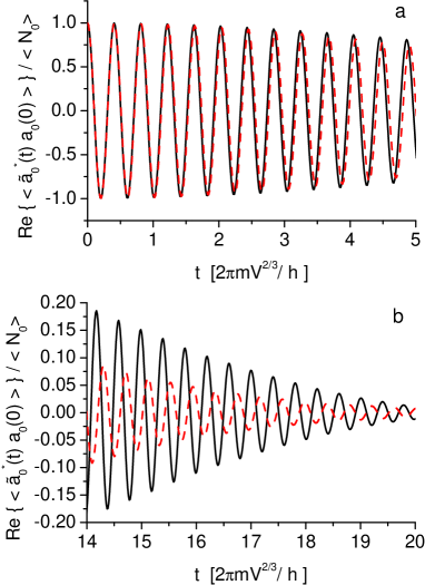
Figure 1: (Color online) Real part of the condensate amplitude correlation function (10) normalized to its $t=0$ value, and divided by the zero temperature evolution $e^{i\rho gt/\hbar}$, as a function of time: in the vertical axis label, $\tilde{a}_{0}(t)$ stands for $a_{0}(t)e^{i\rho gt/\hbar}$. (a) Short times behavior and (b) long times behavior. In solid line from an average over 500 solutions of Eq.(8), in dashed line (red) the Bogoliubov approximation (40). Here the temperature is $k_{B}T=3077.3\,\hbar^{2}/mV^{2/3}=0.1711T_{c}$, where $T_{c}$ is the critical temperature $k_{B}T_{c}=(2\pi\hbar^{2}/m)(\rho/\zeta(3/2))^{2/3}$ of the ideal gas, the number of particles is $N=4\times 10^{5}$ and the coupling constant is such that the zero-temperature chemical potential is $\rho g=gN/V=700\hbar^{2}/mV^{2/3}$.

Correspondingly the standard deviation of the condensate phase change increases with time, as we show in figure 2 for five different values of the temperature, up to $T=0.65T_{c}$. In all cases, at long times, we observe a quadratic growth of $\mbox{Var}\,\varphi$ contrarily to the phase diffusion behavior $\propto t$ predicted in the literature Zoller ; GrahamPRL ; GrahamPRA ; GrahamJMO .

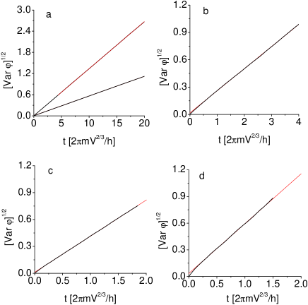
Figure 2: (Color online) Standard deviation of the condensate phase change $\varphi(t)$ (12) as a function of time for (a) $T=0.08245T_{c}$ (lower curve) and $T=0.1711T_{c}$ (upper curve), (b) $T=0.29467T_{c}$, (c) $T=0.453T_{c}$, (d) $T=0.6473T_{c}$. Thick solid line (black): numerical solution from the classical field model Eq.(8) averaged over 500 realizations. Thin solid line (red): a linear fit. The parameters $N$ and $\rho g$ have the same values as in Fig.1.

To complete the physical picture, we show in figure 3 the correlation function of the condensate atom number (11). At very short times, see the beginning of the curves in Fig.3a, the simulation (square symbols) confirms the Bogoliubov prediction (dashed oscillating line); at long times, see Fig.3b, the correlation function drops to a value significantly smaller than the Bogoliubov prediction (fast oscillations are not shown in the figure); a key point is that this long time value of the correlation function of the condensate atom number is not zero.

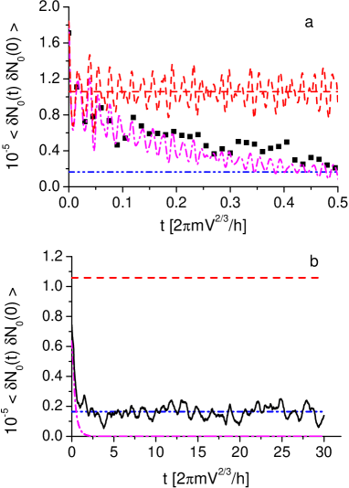
Figure 3: (Color online) Correlation function of the condensate atom number (11). (a) Short times, (b) long times. The classical field results are obtained from an average over 500 solutions of Eq.(8); they are represented by symbols in (a) and a solid line in (b). The dashed lines (red) are the Bogoliubov approximations (21) (oscillating line) and (22) (horizontal line) in (a), and only (22) in (b). The dashed-dotted line (purple) is the Gaussian model. For clarity in (b) we washed out fast oscillations in the simulation result and in the Gaussian model, by averaging over consecutive points over a time width $0.45mV^{2/3}/\hbar$. The horizontal dashed-dotted-dotted line (blue) in (a) and (b) is the ergodic long time limit prediction, described in section IV. The parameters $N$, $T$ and $\rho g$ have the same values as in Fig.1.

One may fear at this stage that the classical field model is missing some source of damping in the dynamics of the system. However it is a well established fact that the classical field model is able to simulate damping processes, including the finite temperature Beliaev-Landau processes Vincent ; Stringari_Pitaevskii ; Giorgini ; Shlyapnikov , since the interaction among the Bogoliubov modes is included in this model Kagan ; Sachdev ; DaliShlyap ; Rzazewski0 ; Burnett ; Cartago ; Rzazewski1 ; Rzazewski2 ; vortex_formation ; bec_collision . More quantitatively we now check that the damping times due to the Beliaev-Landau processes in the simulation are much shorter than the evolution times considered here. To this end, we extract from the simulations the temporal correlation functions $\langle b_{\mathbf{k}}^{*}(t)b_{\mathbf{k}}(0)\rangle$ and $\langle|b_{\mathbf{k}}|^{2}(t)|b_{\mathbf{k}}|^{2}(0)\rangle-\langle|b_{\mathbf{k}}|^{2}\rangle^{2}$, obtained by projecting the classical field over the corresponding Bogoliubov mode and averaging over many realizations. We show these correlation functions for the lowest energy Bogoliubov mode and for an excited Bogoliubov mode in Fig.4.

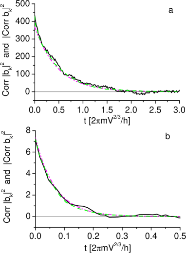
Figure 4: (Color online) Correlation function of $|b_{\mathbf{k}}|^{2}$ (black solid line) and modulus squared of the correlation function of $b_{\mathbf{k}}$ (green dashed line), as obtained from 2000 realisations of the classical field simulations, (a) for the mode ${\bf k}=(0,0,2\pi/L_{3})$ and (b) for the mode ${\bf k}=(2\pi/L_{1},10\pi/L_{2},4\pi/L_{3})$. We define the correlation function of a quantity $X$ as $\mbox{Corr}\,X=\langle X^{*}(t)X(0)\rangle-|\langle X\rangle|^{2}$. The purple dashed-dotted line is an exponential function of $t$, given by Eq.(24). It reproduces well the simulation results, and we have checked that the agreement is good for all vectors ${\bf k}$ lying in an arbitrarily chosen plane in $k$-space. The parameters $N$, $T$ and $\rho g$ have the same values as in Fig.1.

We come then into a paradox. On one side, the various Bogoliubov oscillators $b_{\mathbf{k}}$ decorrelate at long times. On the other side, the variance of the phase change $\varphi$ of the condensate varies quadratically at long times, which implies, as we shall see in Sec. IV, that the derivative of the phase $\dot{\varphi}$ does not decorrelate at long times, although it is a function of the $b_{\mathbf{k}}$’s; similarly, the fluctuations of the number of condensate atoms $\delta N_{0}$, which are functions of the $b_{\mathbf{k}}$’s, do not decorrelate at long times.

This paradox will be explained in Sec. IV, and quantitative predictions for long times behavior of the condensate atom number correlation function and of the variance of the condensate phase change will be derived. Anticipating these analytical results, we show in Fig.5a the long time limit of $(\mbox{Var}\,\varphi)^{1/2}/t$ as a function of $T/T_{c}$, from the results of the classical field simulations, but also from the predictions of the Bogoliubov approximation Eq.(38), and of the ergodic theory of Sec. IV. In figure 5b we show the same results and predictions for the asymptotic value of the condensate atom number correlation function.

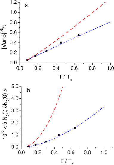
Figure 5: (Color online) (a) Long time limit of $(\mbox{Var}\,\varphi)^{1/2}/t$, in units of $\hbar/mV^{2/3}$, as a function of the temperature over the ideal gas critical temperature. (b) Long time limit of the condensate atom number correlation function, as a function of $T/T_{c}$. In square symbols the numerical results of the classical field simulation (averaged over 500 realizations), in dashed line (red) the Bogoliubov prediction and in dashed-dotted-dotted (blue) the ergodic prediction. The parameters $N$ and $\rho g$ have the same values as in Fig.1.

IV Classical field: Analytical results

The general procedure used here to obtain analytical results is the following. First one expresses the quantity of interest (the number of condensate atoms or the time derivative of the condensate phase) in terms on the amplitudes $b_{\mathbf{k}}$ of the field $\psi$ over the Bogoliubov modes,

$$b_{\mathbf{k}}(t) = dV\sum_{\mathbf{r}}\tilde{U}_{k}\frac{e^{-i\mathbf{k}\cdot\mathbf{r}}}{\sqrt{V}}e^{-i\theta(t)}\psi_{\perp}(\mathbf{r},t)$$ (18)

$$+\tilde{V}_{k}\frac{e^{i\mathbf{k}\cdot\mathbf{r}}}{\sqrt{V}}e^{i\theta(t)}\psi_{\perp}^{*}(\mathbf{r},t)$$

where $\psi_{\perp}$ is the component of $\psi$ orthogonal to the condensate mode. Second one evaluates the correlation functions of products of $b_{\mathbf{k}}$ in various physical limits.

IV.1 Correlation function of the condensate atom number

As the total number of particles is fixed, it is equivalent to calculate the correlation function of $\delta N_{0}$ in Eq.(11) and of the number of non-condensed particles $N_{\perp}$. Injecting the expansion Eq.(14) for the time dependent non-condensed field $\psi_{\perp}$ over the Bogoliubov modes into Eq.(17) we obtain

$$N_{\perp}(t)=\sum_{\mathbf{k}\neq\mathbf{0}}|\tilde{U}_{k}b_{\bf k}(t)+\tilde{V}_{k}b_{\bf-k}^{*}(t)|^{2}.$$ (19)

Bogoliubov theory: In Bogoliubov theory interaction among the Bogoliubov modes is neglected so that at all times

$$b_{\bf k}(t)=b_{\bf k}(0)\,e^{-i\omega_{k}t}\hskip 28.45274pt\mbox{with}\hskip 28.45274pt\omega_{k}=\tilde{\epsilon_{k}}/\hbar\,.$$ (20)

As Wick’s theorem applies for the initial thermal distribution we obtain for the correlation function of the condensate atom number:

$$\langle\delta N_{0}(t)\,\delta N_{0}(0)\rangle_{\rm Bog} = \sum_{\bf k\neq\bf 0}\tilde{n}_{k}^{2}\left[|\tilde{U}_{k}^{2}e^{i\omega_{k}t}+\tilde{V}_{k}^{2}e^{-i\omega_{k}t}|^{2}\right.$$ (21)

$$\left.+(\tilde{U}_{k}\tilde{V}_{k})^{2}|e^{i\omega_{k}t}+e^{-i\omega_{k}t}|^{2}\right]$$

where $\tilde{n}_{k}=k_{B}T/\tilde{\epsilon}_{k}$ is the Bogoliubov mean occupation number of a mode for the classical field. At very short times, a good agreement of the Bogoliubov prediction with the simulation is observed in Fig.3a. Smearing out the terms oscillating rapidly at Bohr frequencies $2\omega_{k}$, we obtain a prediction directly comparable to the coarse grained numerical result of Fig.3b:

$$\langle\delta N_{0}(t)\,\delta N_{0}(0)\rangle_{\rm Bog\;non\,osc}=\sum_{\bf k{\neq}0}(\tilde{U}_{k}^{2}+\tilde{V}_{k}^{2})^{2}\,\tilde{n}_{k}^{2}\,.$$ (22)

This amounts to considering the correlation function of

$$N_{\perp}^{\rm non\ osc}(t)=\sum_{\mathbf{k}\neq\mathbf{0}}(\tilde{U}_{k}^{2}+\tilde{V}_{k}^{2})b_{\mathbf{k}}^{*}(t)b_{\mathbf{k}}(t),$$ (23)

deduced from (19) by eliminating the oscillating terms such as $b_{\mathbf{k}}b_{-\mathbf{k}}$. As can be seen in Fig.3b, Bogoliubov theory fails at long times. Note that in the thermodynamic limit, where the above sum is dominated by the low $k$ terms, one may approximate $\tilde{V}_{k}\sim-\tilde{U}_{k}$, so that Eq.(22) is roughly half of the $t=0$ value of Eq.(21); in other words, it is approximately half of the variance of the condensate number. In the numerical result of Fig.3, the correlation function drops by much more than a factor $2$.

Gaussian theory: A possible approach to improve Bogoliubov theory consists in assuming that the $b_{\mathbf{k}}$ are Gaussian variables with a finite time correlation due to the Beliaev-Landau mechanism:

$$|\langle b_{k}^{\ast}(t)b_{k}(0)\rangle|^{2}=\tilde{n}_{k}^{2}\,e^{-2\gamma_{k}|t|}$$ (24)

where $\gamma_{k}$ is calculated with time dependent perturbation theory including the discrete nature of the spectrum as in Cartago . This amounts to weighting each term of Eq.(22) by $\exp(-2\gamma_{k}|t|)$. This assumption is supported by numerical evidence for a single mode, see Fig.4, and by an analytic derivation in the thermodynamic limit for one or two modes, see Appendix A. Nevertheless, the resulting prediction for the correlation function of $N_{0}$, while looking promising at short times, see Fig.3a, is in clear disagreement with the simulation at long times, see Fig.3b. Since the assumption of a long time decorrelation of $b_{\mathbf{k}}^{*}(t)$ with $b_{\mathbf{k}}(0)$ is physically reasonable, one may suspect that the Gaussian hypothesis is not accurate when a large number of modes are involved as for the correlation function of $N_{0}$. This is indeed the case, as we now show.

Ergodic theory: A systematic way to calculate the long time limit of the correlation function is to assume that the non-linear dynamics generated by Eq.(8) is ergodic: at long times, the $b_{\mathbf{k}}(t)$’s for a given realization of the field explore uniformly a fixed energy surface in phase space moment . In the Bogoliubov approximation for the energy, this means that the $b_{\mathbf{k}}(t)$’s sample the unnormalized probability distribution

$$P_{\infty}(\{b_{\mathbf{k}}\})=\delta\left(E-\sum_{\mathbf{k}\neq\mathbf{0}}\tilde{\epsilon}_{k}b_{\mathbf{k}}^{*}b_{\mathbf{k}}\right)$$ (25)

where the Bogoliubov energy $E$ is fixed by the initial value of the field:

$$E=\sum_{\mathbf{k}\neq\mathbf{0}}\tilde{\epsilon}_{k}b_{\mathbf{k}}^{*}(0)b_{\mathbf{k}}(0).$$ (26)

First, for a given initial condition of the field, we calculate the expectation value of $N_{\perp}(t)$ as given by Eq.(19) over the ergodic distribution Eq.(25), which is equivalent to the temporal average of $N_{\perp}(t)$ over an infinite time interval. The terms of the form $b\,b$ or $b^{*}\,b^{*}$ have a zero mean, since the phases of the $b_{\mathbf{k}}$’s are uniformly distributed over $2\pi$, according to Eq.(25). To calculate the expectation value of the $b^{*}b$ terms, it is convenient to introduce rescaled variables

$$B_{\mathbf{k}}=\left(\frac{\tilde{\epsilon}_{k}}{E}\right)^{1/2}\,b_{\mathbf{k}}.$$ (27)

According to Eq.(25) the real parts and the imaginary parts of all the $B_{\mathbf{k}}$ are uniformly distributed over the unit hypersphere in a space of dimension $2\mathcal{M}$, where $\mathcal{M}=V/dV-1$ is the number of Bogoliubov modes so that we obtain $\overline{|B_{\mathbf{k}}|^{2}}=1/{\mathcal{M}}$ where the overline stands for the average over the ergodic distribution (25). As a consequence the ergodic average of $N_{\perp}$ is

$$\overline{N_{\perp}}=\frac{1}{\mathcal{M}}\sum_{\mathbf{k}\neq\mathbf{0}}(\tilde{U}_{k}^{2}+\tilde{V}_{k}^{2})\frac{E}{\tilde{\epsilon}_{k}}.$$ (28)

Note that this ergodic average depends on the $t=0$ value of the $b_{\mathbf{k}}$’s via (26).

Second, we average the product $\overline{N_{\perp}}\,N_{\perp}(0)$ over the thermal canonical distribution for the initial values $b_{\mathbf{k}}(0)$. This gives the long time limit of the correlation function of the number of condensate atoms:

$$\langle\delta N_{0}(t\rightarrow+\infty)\delta N_{0}(0)\rangle_{\rm ergo}=\frac{1}{\mathcal{M}}\left(\sum_{\mathbf{k}\neq\mathbf{0}}(\tilde{U}_{k}^{2}+\tilde{V}_{k}^{2})\tilde{n}_{k}\right)^{2}.$$ (29)

This prediction is in good agreement with the simulations at long times, see Fig.3b for a fixed value of the temperature, and Fig.5b as a function of temperature. Note that, according to Schwartz inequality, the ergodic value is lower than the coarse grained Bogoliubov prediction Eq.(22), as was expected physically.

This clearly shows that the existence of infinite time correlations in the number of condensate atoms is a consequence of the conservation of energy during the free evolution of the system.

To understand the failure of the Gaussian model, we give the ergodic prediction of the long-time limit of the correlation function of the Bogoliubov mode occupation numbers $n_{\bf k}=|b_{\bf k}|^{2}$,

$$\langle n_{\mathbf{k}}(t\to+\infty)n_{\mathbf{k}^{\prime}}(0)\rangle_{\rm ergo}-\langle n_{\mathbf{k}}\rangle\langle n_{\mathbf{k}^{\prime}}\rangle=\frac{\tilde{n}_{k}\tilde{n}_{k^{\prime}}}{\mathcal{M}}.$$ (30)

This long-time value is non-zero, contrarily to the Gaussian model prediction. One may argue that the value Eq.(30) tends to zero in the thermodynamic limit, so that the error in the Gaussian model looks negligible for a large system. However, in calculating the correlation function of a macroscopic quantity such as $N_{\perp}$, a double sum over the Bogoliubov modes appears, so that the small deviations Eq.(30) from the Gaussian model prediction sum up to a macroscopic value. In other words, in the calculation of a given correlation function, one is not allowed to take the thermodynamic limit before the end of the calculation.

IV.2 Variance of the condensate phase change

To reproduce the approach of the previous subsection for the phase, one should express the phase change $\varphi(t)$ of the condensate amplitude $a_{0}$ as a function of the $b_{\mathbf{k}}$’s. It turns out that the quantity easily expressed in terms of the $b_{\mathbf{k}}$’s is the time derivative $\dot{\varphi}$. The variance of $\varphi$ is then related to the correlation function $\mathcal{C}$ of $\dot{\varphi}$:

$$\mbox{Var}\,{\varphi}=\int_{0}^{t}\,d\tau\,\int_{0}^{t}\,d\tau^{\prime}\,\mathcal{C}(|\tau-\tau^{\prime}|)$$ (31)

where time translational invariance in steady state imposes for a classical field that ${\cal C}$ depends only on $|\tau-\tau^{\prime}|$:

$${\cal C}(|\tau-\tau^{\prime}|)=\langle\dot{\varphi}(\tau)\dot{\varphi}(\tau^{\prime})\rangle-\langle\dot{\varphi}(\tau)\rangle\langle\dot{\varphi}(\tau^{\prime})\rangle\,.$$ (32)

If $\mathcal{C}(\tau)\rightarrow 0$ fast enough when $\tau\rightarrow\infty$ then $\mbox{Var}\,{\varphi}$ grows linearly in time. On the other hand, if $\mathcal{C}(\tau)$ has a non-zero limit at long times, then $\mbox{Var}\,{\varphi}$ grows quadratically in time fastenought .

To express $\dot{\varphi}$ in terms of the $b_{\mathbf{k}}$’s, we write the equation of motion for $a_{0}$:

$$i\hbar\dot{a}_{0} = i\hbar\{a_{0},H\}=\partial_{a_{0}^{*}}H$$ (33)

$$= \frac{g}{\sqrt{V}}\sum_{\mathbf{r}}\psi^{*}(\mathbf{r})\psi^{2}(\mathbf{r})$$

where we used $\partial_{a_{0}^{*}}\psi^{*}(\mathbf{r})=1/\sqrt{V}$ obtained from Eq.(2). We split $\psi$ as in Eq.(16); we eliminate the condensate amplitude in the resulting expression for $\dot{a}_{0}/a_{0}$ (i) by using $|a_{0}|^{2}=N-N_{\perp}$, where $N_{\perp}$ is a function of the $b_{\mathbf{k}}$’s, see Eq.(19), and (ii) by introducing the field CastinDum

$$\Lambda({\bf r})=e^{-i\,\theta}\psi_{\perp}({\bf r})$$ (34)

which is a function of the $b_{\mathbf{k}}$’s only according to Eq.(14). This leads to

$$i\hbar\frac{\dot{a_{0}}}{a_{0}} = \rho g+\frac{g}{V}\sum_{\bf r}dV\left[\Lambda({\bf r})^{2}+|\Lambda({\bf r})|^{2}\right]$$ (35)

$$+ \frac{g}{\sqrt{V}}\sum_{\bf r}dV\frac{\Lambda^{*}({\bf r})\Lambda^{2}({\bf r})}{\sqrt{N-N_{\perp}}}.$$

The real part of the above equation gives $-\hbar\dot{\theta}$, which is also $-\hbar\dot{\varphi}$.

Restricting to a weak non-condensed fraction, we drop the cubic terms in Eq.(35), to obtain notN0

$$\hbar\dot{\varphi} \simeq -\rho g-\frac{1}{2}\frac{g}{V}\sum_{\bf r}dV\left[\Lambda({\bf r})+\Lambda^{*}({\bf r})\right]^{2}$$ (36)

$$= -\rho g-\frac{1}{2}\frac{g}{V}\sum_{\mathbf{k}\neq\mathbf{0}}\,(\tilde{U}_{k}+\tilde{V}_{k})^{2}\,|b_{\bf k}+b_{\bf-k}^{\ast}|^{2}.$$

It turns out that the products $b_{\bf k}b_{\bf-k}$ generate oscillating terms which do not contribute to a coarse grained time average. It is thus useful to define

$$\hbar\dot{\varphi}_{\rm non\ osc}=-\rho g-\frac{g}{V}\sum_{\mathbf{k}\neq\mathbf{0}}\,(\tilde{U}_{k}+\tilde{V}_{k})^{2}\,|b_{\bf k}|^{2}.$$ (37)

Bogoliubov theory: By using (20) and Wick’s theorem we calculate the correlation function of Eq.(36). By temporal integration we obtain the variance of the condensate phase change

$$(\mbox{Var}\,{\varphi})_{\rm Bog}=\left(\frac{g}{\hbar V}\right)^{2}\sum_{\mathbf{k}\neq\mathbf{0}}(\tilde{U}_{k}+\tilde{V}_{k})^{4}\,\tilde{n}_{k}^{2}\,\left[t^{2}+\frac{\sin^{2}\omega_{k}t}{(2\omega_{k})^{2}}\right]\,.$$ (38)

Qualitatively Bogoliubov theory correctly predicts a quadratic growth of the variance of $\varphi$ at long times. As we show in Fig.5a, however, it is not fully quantitative: it does not reproduce the value of the dephasing rate obtained from the simulations. This is not surprising as in the full non linear theory the $b_{\bf k}$’s interact and do not follow Eq.(20).

To be complete, we also give the Bogoliubov approximation for the correlation function of the condensate amplitude $a_{0}$. Neglecting the fluctuations of the modulus of $a_{0}$, one can set

$$\langle a_{0}^{\ast}(t)\,a_{0}(0)\rangle\simeq\langle N_{0}\rangle\langle e^{-i\,\varphi(t)}\rangle\,.$$ (39)

Dropping the oscillating terms in $b_{\bf k}b_{\bf-k}$ and $b^{*}_{\bf k}b^{*}_{\bf-k}$ in $\dot{\varphi}(t)$, which give a small contribution, we get

$$\langle a_{0}^{\ast}(t)\,\hat{a}_{0}(0)\rangle_{\rm Bog}\simeq\langle N_{0}\rangle\prod_{\mathbf{k}\neq\mathbf{0}}\frac{1}{1+i\frac{g}{\hbar V}(\tilde{U}_{k}+\tilde{V}_{k})^{2}\,\tilde{n}_{k}\,t}\,.$$ (40)

The resulting expression is plotted as a dashed line in Fig.1 against the result of the simulation.

Gaussian theory: If we add by hand a decorrelation of the $b_{\bf k}$’s and assume Gaussian statistics, we get a diffusive spreading of the condensate phase change, with the variance of $\varphi_{\rm non\ osc}$ growing linearly at long times:

$$(\mbox{Var}\,\varphi)_{\rm Gauss}=\left(\frac{g}{\hbar V}\right)^{2}\sum_{\mathbf{k}\neq\mathbf{0}}(\tilde{U}_{k}+\tilde{V}_{k})^{4}\,\tilde{n}_{k}^{2}\,\left[\frac{e^{-2\gamma_{k}t}-1}{2\gamma_{k}^{2}}+\frac{t}{\gamma_{k}}\right]\,,$$ (41)

in clear contradiction with the numerical simulations. This prediction corresponds to a correlation function $\mathcal{C}$ vanishing at long times, whereas the correct correlation function has a finite limit, see Fig.6.

Ergodic theory: as in subsection IV.1 we calculate the long time value of the correlation function for $\dot{\varphi}$ using the ergodic assumption. The various steps of the calculation are rigorously the same as in Sec. IV.1 and lead to

$$\mathcal{C}(\tau\rightarrow+\infty)_{\rm ergo}=\left(\frac{g}{\hbar V}\right)^{2}\frac{1}{\mathcal{M}}\left(\sum_{\mathbf{k}\neq\mathbf{0}}(\tilde{U}_{k}+\tilde{V}_{k})^{2}\tilde{n}_{k}\right)^{2}.$$ (42)

This prediction is in excellent agreement with the simulations: it gives the correct asymptotic value of $\mathcal{C}$, see Fig.6, and from the asymptotic expression $\mbox{Var}\,\varphi\simeq\mathcal{C}(+\infty)t^{2}$ it gives the correct values of the long time limit of $(\mbox{Var}\,\varphi)^{1/2}/t$, see Fig.5a, as a function of temperature.

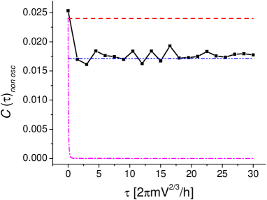
Figure 6: (Color online) Correlation function ${\cal C}_{\rm non\ osc}$ of the quantity $\dot{\varphi}_{\rm non\ osc}$ defined in Eq.(37) calculated from the simulation (square symbols; the solid line is a guide to the eye), or using the Gaussian theory (purple dashed-dotted line going to zero at long times). In dashed line (red) the Bogoliubov prediction. In dashed-dotted-dotted line (blue) the long time prediction (42) of the ergodic theory. The parameters $T$, $N$ and $\rho g$ have the same values as in Fig.1.

V Quantum Treatment: Analytical Results

So far the classical field model was very useful in revealing the physical processes governing the long time behavior of the phase and atom number fluctuations in the condensate. However it is not a fully quantitative theory, as the long time limits of the correlation functions considered here depend on the precise choice of the energy cut-off, that is on the number of Bogoliubov modes $\mathcal{M}$ in the simulation, as is apparent on Eqs.(29,42). In this section, we therefore adapt the previous physical reasonings to the quantum field case.

V.1 The quantum model

We use a straightforward generalization of the classical field lattice model, taking here for simplicity a cubic lattice, as discussed in les_houches ; Cartago ; Mora . The bosonic field $\hat{\psi}$ evolves according to the Hamiltonian

$$H=\sum_{\mathbf{k}}\frac{\hbar^{2}k^{2}}{2m}\,\hat{a}_{\mathbf{k}}^{\dagger}\hat{a}_{\mathbf{k}}+\frac{g_{0}}{2}\sum_{\mathbf{r}}dV\,\hat{\psi}^{\dagger}\hat{\psi}^{\dagger}\hat{\psi}\hat{\psi},$$ (43)

where $\hat{a}_{\mathbf{k}}$ annihilates a particle of wavevector $\mathbf{k}$ in the first Brillouin zone. The dispersion relation of the wave is now the usual one. The total number of atoms is fixed, equal to $N$. The coupling constant $g_{0}$ depends on the lattice spacing $l$ in order to ensure a $l$-independent scattering length for the discrete delta interaction potential among the particles Mora ; les_houches :

$$V(\mathbf{r}_{1}-\mathbf{r}_{2})=\frac{g_{0}}{dV}\delta_{\mathbf{r}_{1},\mathbf{r}_{2}}.$$ (44)

Since we consider here the weakly interacting regime, we can restrict to a lattice spacing much larger than the scattering length $a$ so that $g_{0}$ is actually very close to $g=4\pi\hbar^{2}a/m$.

To be able to use Bogoliubov theory as we did in the classical field reasoning, we restrict to the low temperature regime $T\ll T_{c}$ with a macroscopic occupation of the condensate mode. We thus neglect the possibility that the condensate is empty, which allows us to use the modulus-phase representation of the condensate mode:

$$\hat{a}_{0}\simeq e^{i\hat{\theta}}\sqrt{\hat{N}_{0}}$$ (45)

where $\hat{N}_{0}=\hat{a}_{0}^{\dagger}\hat{a}_{0}$ and where $\hat{\theta}$ is a Hermitian ‘phase’ operator obeying the commutation relation

$$[\hat{N}_{0},\hat{\theta}]=i.$$ (46)

This allows to consider the correlation of the condensate atom number fluctuation $\delta\hat{N}_{0}\equiv\hat{N}_{0}-\langle\hat{N}_{0}\rangle$ but also the variance of the condensate phase change $\hat{\varphi}(t)\equiv\hat{\theta}(t)-\hat{\theta}(0)$, as we did for the classical field.

V.2 Correlation function of the condensate atom number

To predict the correlation function of $\delta\hat{N}_{0}$, we use Bogoliubov theory at short times and the quantum analog of the ergodic theory at long times.

In the number conserving Bogoliubov theory Gardiner ; CastinDum , written here for a spatially homogeneous system, one introduces the field conserving the total number of particles

$$\hat{\Lambda}(\mathbf{r})\equiv e^{-i\hat{\theta}}\hat{\psi}_{\perp}(\mathbf{r})$$ (47)

where the non-condensed field $\hat{\psi}_{\perp}$ is obtained by projecting out the component of the field $\hat{\psi}$ on the condensate mode. The field $\hat{\Lambda}$ then admits the modal expansion on the Bogoliubov modes

$$\hat{\Lambda}(\mathbf{r})=\sum_{\mathbf{k}\neq\mathbf{0}}\hat{b}_{\mathbf{k}}U_{k}\frac{e^{i\mathbf{k}\cdot\mathbf{r}}}{\sqrt{V}}+\hat{b}^{\dagger}_{\mathbf{k}}V_{k}\frac{e^{-i\mathbf{k}\cdot\mathbf{r}}}{\sqrt{V}}$$ (48)

where the real amplitudes $U_{k}$, $V_{k}$, normalized as $U_{k}^{2}-V_{k}^{2}=1$, are given by the usual Bogoliubov theory,

$$U_{k}+V_{k}=\left(\frac{\hbar^{2}k^{2}/2m}{2\rho g_{0}+\hbar^{2}k^{2}/2m}\right)^{1/4}.$$ (49)

Since the total number of particles is fixed to $N$, it is equivalent to consider the fluctuations of $\hat{N}_{0}$ or of the number of non-condensed atoms

$$\hat{N}_{\perp}=\sum_{\mathbf{r}}dV\hat{\Lambda}^{\dagger}(\mathbf{r})\hat{\Lambda}(\mathbf{r}).$$ (50)

This, together with the expansion (48), expresses $\hat{N}_{\perp}$ as a function of the $\hat{b}_{\mathbf{k}}$’s.

The equilibrium state of the system is approximated in the canonical ensemble by the Bogoliubov thermal density operator

$$\hat{\rho}_{\rm Bog}(T)=\frac{1}{Z_{\mathrm{Bog}}}e^{-\sum_{\mathbf{k}\neq\mathbf{0}}\epsilon_{k}\hat{b}^{\dagger}_{\mathbf{k}}\hat{b}_{\mathbf{k}}/k_{B}T}$$ (51)

where the normalization factor $Z_{\mathrm{Bog}}$ is the Bogoliubov approximation for the partition function, and where we have introduced the Bogoliubov spectrum

$$\epsilon_{k}=\left[\frac{\hbar^{2}k^{2}}{2m}\left(\frac{\hbar^{2}k^{2}}{2m}+2\rho g_{0}\right)\right]^{1/2}.$$ (52)

Bogoliubov theory: In the Bogoliubov approximation for the time evolution, the $\hat{b}_{\mathbf{k}}$ merely accumulate a phase, at the frequency $\omega_{k}=\epsilon_{k}/\hbar$, similarly to the classical field case. From Wick’s theorem one then obtains

$$\frac{1}{2}\langle\{\delta\hat{N}_{0}(t),\delta\hat{N}_{0}(0)\}\rangle_{\rm Bog}=\sum_{\bf k\neq\bf 0}\bar{n}_{k}(\bar{n}_{k}+1)(U_{k}^{2}+V_{k}^{2})^{2}$$

$$+2U_{k}^{2}V_{k}^{2}\cos(2\omega_{k}t)\,[\bar{n}_{k}^{2}+(\bar{n}_{k}+1)^{2}]$$ (53)

where

$$\bar{n}_{k}(T)=\frac{1}{\exp(\epsilon_{k}/k_{B}T)-1}$$ (54)

is the mean occupation number of the Bogoliubov mode $\mathbf{k}$. Note that we have considered here the so-called symmetric correlation function (as $\{X,Y\}$ stands for the anticommutator $XY+YX$ of two operators) which is a real quantity, equal to the real part of the non-symmetrized correlation function. The time coarse grained version of the prediction (53) is obtained by averaging out the oscillating terms, which amounts to considering the correlation function of the temporally smoothed operator number of non-condensed particles

$$\hat{N}_{\perp}^{\rm non\ osc}\equiv\sum_{\mathbf{k}\neq\mathbf{0}}\left[\left(U_{k}^{2}+V_{k}^{2}\right)\hat{b}_{\mathbf{k}}^{\dagger}\hat{b}_{\mathbf{k}}+V_{k}^{2}\right].$$ (55)

Quantum Ergodic theory: Discarding from the start the oscillating terms in $\hat{N}_{\perp}$, as in (55), we face here the problem of calculating the long time limit of $\langle A(t)A(0)\rangle$, where $A$ is a linear function of the Bogoliubov mode occupation numbers,

$$A=\sum_{\mathbf{k}\neq\mathbf{0}}\gamma_{k}\hat{b}^{\dagger}_{\mathbf{k}}\hat{b}_{\mathbf{k}}\,.$$ (56)

As the quantum state of the system is given by the Bogoliubov approximation Eq.(51), we may inject a closure relation in the Bogoliubov Fock eigenbasis:

$$\langle A(t)A(0)\rangle = \frac{1}{Z_{\mathrm{Bog}}}\sum_{\{n_{\mathbf{k}}\}}e^{-\beta\sum_{\mathbf{k}\neq\mathbf{0}}\epsilon_{k}n_{\mathbf{k}}}\left(\sum_{\mathbf{k}\neq\mathbf{0}}\gamma_{k}n_{\mathbf{k}}\right)$$ (57)

$$\times\langle\{n_{\mathbf{k}}\}|A(t)|\{n_{\mathbf{k}}\}\rangle,$$

where the sum is taken over all possible integer values of the occupation numbers, not to be confused with the mean occupation numbers (54).

The non-explicit piece of this expression is the matrix element of $A(t)$, which may be reinterpreted as follows:

$$\langle\{n_{\mathbf{k}}\}|A(t)|\{n_{\mathbf{k}}\}\rangle=\mbox{Tr}\,\left[A\sigma(t)\right]$$ (58)

where the density operator $\sigma$, initially a pure state in the Bogoliubov Fock basis,

$$\sigma(0)=|\{n_{\mathbf{k}}\}\rangle\langle\{n_{\mathbf{k}}\}|$$ (59)

evolves during $t$ with the full Hamiltonian $H$. We know that this evolution involves Beliaev-Landau processes that will spread $\sigma$ over the various Fock states $|\{n^{\prime}_{\mathbf{k}}\}\rangle$. This evolution is complex. But we need here the long time limit only, in which we may assume that an equilibrium statistical description is possible. Since the system is isolated during its evolution, we take for $\sigma(t\to+\infty)$ the equilibrium density operator in the microcanonical ensemble Deutsch , and we calculate the expectation value of $A$ with $\sigma(t\to+\infty)$ as we did for the classical field model. The calculation can be done in the thermodynamic limit. As shown in the Appendix B, one can calculate to leading order in this limit the difference between canonical and microcanonical averages.

Here the microcanonical ensemble has an energy $E=E_{0}^{\rm Bog}+\sum_{\mathbf{k}\neq\mathbf{0}}\epsilon_{k}n_{\mathbf{k}}$, where $E_{0}^{\rm Bog}$ is the ground state Bogoliubov energy. We introduce the effective temperature $T_{\rm eff}$ such that the mean energy in the canonical ensemble at temperature $T_{\rm eff}$ is equal to $E$,

$$0=\langle H_{\rm Bog}\rangle(T_{\rm eff})-E=\sum_{\mathbf{k}\neq\mathbf{0}}\epsilon_{k}[\bar{n}_{k}(T_{\rm eff})-n_{\mathbf{k}}]$$ (60)

where $\langle\ldots\rangle$ stands for an average in the canonical ensemble and $H_{\rm Bog}$ is the Bogoliubov Hamiltonian. Using the results of Appendix B one gets

$$\bar{A}(E)-\langle A\rangle(T_{\rm eff})=-\frac{1}{2}k_{B}T_{\rm eff}^{2}\left(\frac{\langle A\rangle^{\prime}}{\langle H_{\rm Bog}\rangle^{\prime}}\right)^{\prime}(T_{\rm eff})$$ (61)

where $\bar{A}(E)$ is the microcanonical average of $A$ at energy $E$ and where the apex ^′ stands for derivation with respect to temperature. We further use the fact that, in the thermodynamic limit, for typical values of the occupation numbers $n_{\mathbf{k}}$, $T_{\rm eff}$ weakly deviates from the physical temperature $T$. We calculate $T_{\rm eff}$ by expanding (60) up to second order in $T_{\rm eff}-T$ more_details . Evaluating (61) with this value of $T_{\rm eff}$, keeping terms up to the relevant order more_details , gives the desired result

$$\langle\{n_{\mathbf{k}}\}|A(t\rightarrow+\infty)|\{n_{\mathbf{k}}\}\rangle=\langle A\rangle$$ (62)

$$+ \left[\sum_{\mathbf{k}\neq\mathbf{0}}\epsilon_{k}(n_{\mathbf{k}}-\bar{n}_{k})\right]\frac{\langle A\rangle^{\prime}}{\langle H_{\rm Bog}\rangle^{\prime}}+\frac{1}{2}\left(\frac{\langle A\rangle^{\prime}}{\langle H_{\rm Bog}\rangle^{\prime}}\right)^{\prime}$$

$$\times \left\{\frac{\left[\sum_{\mathbf{k}\neq\mathbf{0}}\epsilon_{k}(n_{\mathbf{k}}-\bar{n}_{k})\right]^{2}}{\langle H_{\rm Bog}\rangle^{\prime}}-k_{B}T^{2}\right\}$$

where all the canonical averages are now evaluated at the physical temperature $T$ check .

It remains to inject this expression into Eq.(57). The resulting average over $n_{\bf k}$ leads to the long time value of the correlation function:

$$\langle A(+\infty)A(0)\rangle-\langle A\rangle^{2} = \left(\frac{\langle A\rangle^{\prime}}{\langle H_{\rm Bog}\rangle^{\prime}}\right)^{2}{\rm Var}\,H_{\rm Bog}$$ (63)

$$= \frac{\left[\sum_{\mathbf{k}\neq\mathbf{0}}\gamma_{k}\epsilon_{k}\bar{n}_{k}(\bar{n}_{k}+1)\right]^{2}}{\sum_{\mathbf{k}\neq\mathbf{0}}\epsilon_{k}^{2}\bar{n}_{k}(\bar{n}_{k}+1)},$$ (64)

where we used Wick theorem and the property $d\bar{n}_{k}/dT=\epsilon_{k}\bar{n}_{k}(\bar{n}_{k}+1)/k_{B}T^{2}$ troisieme . Using Schwartz inequality, one can show that this long time value of the correlation function is less than its zero time value $\sum\gamma_{k}^{2}\bar{n}_{k}(\bar{n}_{k}+1)$. To be complete, we present an alternative derivation of our prediction (64) in the Appendix C, based on results obtained in Deutsch . We also note that the quantum ergodic calculation directly leads to a prediction of the long time limit for the correlation function of the Bogoliubov mode occupation numbers, see Eq.(95).

Replacing in Eq.(64) the coefficients $\gamma_{k}$ by their expression from Eq.(55), $\gamma_{k}=U_{k}^{2}+V_{k}^{2}$, we obtain the long time value of the condensate atom number correlation function in the quantum ergodic theory. Note that, in the thermodynamic limit, this long time value scales as the volume $V$, whereas the $t=0$ value scales as $V^{4/3}$.

V.3 Correlation function of the time derivative of the condensate phase

As in the classical field case, we first look for an expression of the first order time derivative of the condensate phase operator $\hat{\theta}$ in terms of the amplitudes of the field $\hat{\Lambda}$ on the Bogoliubov modes. Taking as a starting point in Heisenberg picture

$$i\hbar\frac{d}{dt}\hat{\theta}=[\hat{\theta},H],$$ (65)

we split the quantum field in a condensate part and a non-condensed part,

$$\hat{\psi}(\mathbf{r})=\frac{\hat{a}_{0}}{\sqrt{V}}+\hat{\psi}_{\perp}(\mathbf{r}),$$ (66)

and we insert this splitting in the expression of $H$. Using the modulus-phase representation of $\hat{a}_{0}$ and the commutation relation Eq.(46), we obtain, using $\hat{a}_{0}^{\dagger}\hat{a}_{0}=\hat{N}-\hat{N}_{\perp}$,

$$-\hbar\frac{d}{dt}\hat{\theta} = \frac{g_{0}}{V}\left[\hat{N}-\frac{1}{2}+\sum_{\mathbf{r}}dV\hat{\Lambda}^{\dagger}\hat{\Lambda}\right]$$ (67)

$$+ \frac{g_{0}}{2V}\sum_{\mathbf{r}}dV\left[\hat{\Lambda}\frac{\hat{N}_{0}+1/2}{\sqrt{\hat{N}_{0}(\hat{N}_{0}+1)}}\hat{\Lambda}+\mbox{h.c.}\right]$$

$$+ \frac{g_{0}}{2\sqrt{V}}\sum_{\mathbf{r}}dV\,\left[\frac{1}{\sqrt{\hat{N}_{0}}}\,\hat{\Lambda}^{\dagger}\hat{\Lambda}^{2}+\mbox{h.c.}\right].$$

The quantity $(\hat{N}_{0}+1/2)/\sqrt{\hat{N}_{0}(\hat{N}_{0}+1)}$ is actually $1+O(1/\hat{N}_{0}^{2})$ so it can to a high accuracy be replaced by unity. Furthermore, as we did in the classical field model, we now keep the leading terms in $\hat{\Lambda}$, under the assumption of a weak non-condensed fraction. We can also replace $\hat{\theta}$ by $\hat{\varphi}$ under the temporal derivative, since $\hat{\theta}(0)$ is time independent. We obtain notN0

$$-\hbar\frac{d}{dt}\hat{\varphi}\simeq\frac{g_{0}}{V}\left[\hat{N}-\frac{1}{2}+\sum_{\mathbf{r}}dV\left(\hat{\Lambda}^{\dagger}\hat{\Lambda}+\frac{1}{2}\hat{\Lambda}^{2}+\frac{1}{2}\hat{\Lambda}^{\dagger 2}\right)\right].$$ (68)

Taking the expectation value of this expression over the thermal state in the Bogoliubov approximation leads to an expression coinciding with the value of the chemical potential predicted by Eq.(103) of Mora , which includes in a systematic way the first correction to the pure condensate prediction $\rho g_{0}$ more_precisely :

$$\mu(T)=\frac{g_{0}}{V}\left[N-\frac{1}{2}+\sum_{\mathbf{k}\neq\mathbf{0}}(U_{k}+V_{k})^{2}\bar{n}_{k}+V_{k}(U_{k}+V_{k})\right].$$ (69)

At this order of the expansion, this analytically shows that $-\hbar\langle d\hat{\theta}/dt\rangle$ is the chemical potential of the system. We now turn to various predictions for the symmetrized correlation function of $d\hat{\varphi}/dt$,

$$\mathcal{C}_{\rm S}(\tau)=\frac{1}{2}\Big{\langle}\left\{\left(\frac{d}{dt}\hat{\varphi}\right)(\tau),\left(\frac{d}{dt}\hat{\varphi}\right)(0)\right\}\Big{\rangle}-\langle\frac{d}{dt}\hat{\varphi}\rangle^{2}.$$ (70)

Bogoliubov theory: At a time short enough for the interactions between the Bogoliubov modes to remain negligible, one can apply Bogoliubov theory to get

$$\mathcal{C}_{\rm S}^{\rm Bog}(\tau) = \left(\frac{g_{0}}{\hbar V}\right)^{2}\sum_{\mathbf{k}\neq\mathbf{0}}(U_{k}+V_{k})^{4}\left\{\bar{n}_{k}(\bar{n}_{k}+1)\phantom{\frac{a^{b}}{c^{d}}}\right.$$ (71)

$$+ \left.\frac{1}{2}\cos(2\omega_{k}t)\left[\bar{n}_{k}^{2}+(\bar{n}_{k}+1)^{2}\right]\right\}.$$

The temporal coarse grained version of this correlation function is obtained by averaging out the cosine terms, which amounts to considering a temporal derivative of $\hat{\varphi}$ freed from the oscillating terms $\hat{b}\hat{b}$ and $\hat{b}^{\dagger}\hat{b}^{\dagger}$:

$$\left(\frac{d}{dt}\hat{\varphi}\right)_{\rm nonosc} = -\frac{g_{0}}{\hbar V}\left[\hat{N}-\frac{1}{2}+\sum_{\mathbf{k}\neq\mathbf{0}}V_{k}(U_{k}+V_{k})\right]$$ (72)

$$- \frac{g_{0}}{\hbar V}\sum_{\mathbf{k}\neq\mathbf{0}}(U_{k}+V_{k})^{2}\hat{b}^{\dagger}_{\mathbf{k}}\hat{b}_{\mathbf{k}}.$$

Quantum ergodic theory: We directly apply to the smoothed temporal derivative (72) the reasoning performed in the previous subsection. Up to an additive constant, Eq.(72) is indeed of the form (56), with $\gamma_{k}=-(g_{0}/\hbar V)(U_{k}+V_{k})^{2}$. From (64) we therefore obtain the long time behavior of the phase derivative correlation function

$$\mathcal{C}_{\rm S}^{\rm ergo}(+\infty)=\left(\frac{g_{0}}{\hbar V}\right)^{2}\frac{\left[\sum_{\mathbf{k}\neq\mathbf{0}}(U_{k}+V_{k})^{2}\epsilon_{k}\bar{n}_{k}(\bar{n}_{k}+1)\right]^{2}}{\sum_{\mathbf{k}\neq\mathbf{0}}\epsilon_{k}^{2}\bar{n}_{k}(\bar{n}_{k}+1)}.$$ (73)

The long time limit of the variance of the phase difference is then comp_clas

$${\rm Var}\,\hat{\varphi}\sim\mathcal{C}_{\rm S}^{\rm ergo}(+\infty)t^{2}\,.$$ (74)

Although our conclusion of a ballistic behavior for the phase agrees qualitatively with Kuklov , the explicit expression of the coefficient of $t^{2}$ differs from the one of Kuklov due the fact that we account for interactions among Bogoliubov modes such as the Beliaev-Landau processes leading to ergodicity in the system, while in Kuklov the many-body Hamiltonian is replaced by the Bogoliubov Hamiltonian in the last stage of the calculation. As can be seen from (73) using Schwartz inequality, ergodicity results in a reduction of phase fluctuations with respect to the Bogoliubov prediction.

In the thermodynamic limit, analytical expressions can be obtained for this ergodic prediction. In the low temperature limit $k_{B}T\ll\rho g$,

$$\mathcal{C}_{\rm S}^{\rm ergo}(+\infty)\sim\frac{8\pi^{4}}{15}\frac{a^{2}\xi}{V}\left(\frac{k_{B}T}{\hbar}\right)^{2}\left(\frac{k_{B}T}{\rho g}\right)^{3},$$ (75)

where $\xi$ is the healing length such that $\hbar^{2}/m\xi^{2}=\rho g$. This tends to zero at zero temperature comp_to_Beliaev . In the high temperature limit $k_{B}T\gg\rho g$,

$$\mathcal{C}_{\rm S}^{\rm ergo}(+\infty)\sim\frac{12\zeta(3/2)^{2}}{5\zeta(5/2)}\frac{a^{2}\lambda}{V}\left(\frac{k_{B}T}{\hbar}\right)^{2}$$ (76)

where the thermal de Broglie wavelength obeys $\lambda^{2}=2\pi\hbar^{2}/mk_{B}T$ and where $\zeta$ is the Riemann Zeta function. Here we have identified $g_{0}$ to $g$ amusing . In Fig.7 we give the quantum ergodic prediction for $\lim_{t\to\infty}(\mbox{Var}\,\hat{\varphi})^{1/2}/t$ calculated numerically, which is a universal function of $k_{B}T/\rho g$ when expressed in the right units.

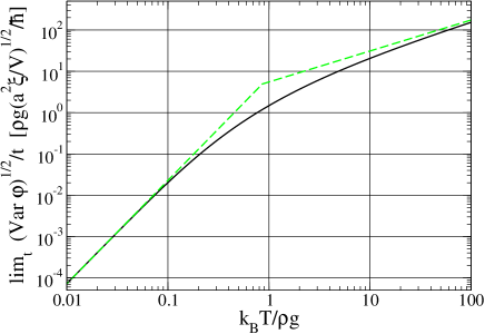
Figure 7: (Color online) In the regime $T\ll T_{c}$ for a weakly interacting Bose gas, quantum ergodic prediction (73) for the long time limit of $(\mbox{Var}\,\hat{\varphi})^{1/2}/t$, in the thermodynamic limit. When expressed in units of $(a^{2}\xi/V)^{1/2}\rho g/\hbar$, $(\mbox{Var}\,\hat{\varphi})^{1/2}/t$ is a function of $k_{B}T/\rho g$ only, that is readily calculated numerically (solid line) or that may be approximated by asymptotic equivalents (75,76) in the low temperature or high temperature limit (green dashed line). Note that the dimensionless quantity $a^{2}\xi/V$ may also be written as $\sqrt{\rho a^{3}}/(N\sqrt{4\pi})$.

VI Conclusion

We have investigated theoretically the phase spreading of a finite temperature weakly interacting condensate. The gas is assumed to be prepared at thermal equilibrium in the canonical ensemble, and then to freely evolve as an isolated system. After average over many realizations of the system, we find in classical field simulations that the variance $\mbox{Var}\,\varphi$ of the condensate phase change grows quadratically in time. This non-diffusive behavior is quantitatively explained by an ergodic theory for the Bogoliubov modes, the key point being that conservation of energy during the free evolution prevents some correlation functions of the field from vanishing at long times. We have extended the analytical treatment to the quantum field case and we have determined the coefficient of the $t^{2}$ term in the long time behavior of $\mbox{Var}\,\hat{\varphi}$, see Eq.(73). This analytical result holds at low temperature $T\ll T_{c}$ and in the weakly interacting regime $\rho a^{3}\ll 1$, for a large number of thermally populated Bogoliubov modes, and relies on the assumption that the (although weak) interaction among the Bogoliubov modes efficiently mixes them (quantum ergodic regime).

A physical insight in our result is obtained from the following rewriting

$$\mbox{Var}\,\hat{\varphi}(t)\sim\frac{t^{2}}{\hbar^{2}}\left(\frac{\partial_{T}\mu}{\partial_{T}\langle H\rangle}\right)^{2}\mbox{Var}\,H$$ (77)

where $\mbox{Var}\,H$ is the variance of the energy of the gas, here in the Bogoliubov approximation and in the canonical ensemble, $\mu(T)$ is the chemical potential of the system as given by Eq.(69) and $\langle H\rangle(T)$ is its mean energy in the Bogoliubov approximation.

This formula may also be obtained from the following reasoning. For a given realization of the system, of energy $E$, the long time limit of the condensate phase change $\hat{\varphi}(t)$ can be shown to behave as

$$\hat{\varphi}(t)\sim-\mu_{\rm micro}(E)t/\hbar,$$ (78)

where $\mu_{\rm micro}$ is the chemical potential calculated in the microcanonical ensemble proof . For a large system, canonical energy fluctuations around the mean energy $\langle H\rangle(T)$ are weak in relative value so that one may expand $\mu_{\rm micro}(E)$ to first order in $E-\langle H\rangle$. Taking the variance of $\hat{\varphi(t)}$ over the canonical fluctuations of $E$ then leads to (77), since $\partial_{T}\mu/\partial_{T}\langle H\rangle\simeq\partial_{E}\mu_{\rm micro}(\langle H\rangle)$ for a large system.

This reasoning shows that a necessary condition for the observation of an intrinsic diffusive spreading of the condensate phase change is a strong suppression of the energy fluctuations of the gas. To this end one may try to prepare the system in a clever way, starting with a pure condensate and giving to the system a well defined amount of energy, e.g. by a reproducible change of the trapping potential Thomas . Alternatively one may try to follow a given experimental realization of the system, measuring the phase of the condensate in a non-destructive way and replacing ensemble average by time average.

We thank Fabrice Gerbier and Li Yun for useful comments on the manuscript, and Mikhail Kolobov for interest in the problem. We thank Francis Hulin-Hubard for giving us access to a multiprocessor machine. We are grateful to Anatoly Kuklov for pointing to us his work Kuklov and for useful discussions. One of us (E. W.) acknowledges financial support from QuFAR. Laboratoire Kastler Brossel is a research unit of University Paris 6 and Ecole normale supérieure, associated to CNRS. Our group is a member of IFRAF.

Appendix A Temporal correlation function of the Bogoliubov mode occupation numbers

Using the master equation approach developed in quantum optics Louisell ; CCT , we calculate the temporal correlation function of the operator $\hat{b}_{\mathbf{q}}^{\dagger}\hat{b}_{\mathbf{q}}$ giving the number of Bogoliubov excitations in the mode of wavevector $\mathbf{q}$, in the thermodynamic limit and including the Beliaev-Landau coupling among the Bogoliubov modes. This is useful to motivate the Gaussian model introduced in section IV, and to estimate the time required for the correlation function $\langle A(t)A(0)\rangle-\langle A\rangle^{2}$, where $A$ is of the form Eq.(56), to depart from its value predicted by the Bogoliubov theory.

The idea of the master equation approach is to split the whole system in a small system $S$ and a large reservoir $R$ with a continuous energy spectrum. Treating the coupling $W$ between $S$ and $R$ in the Born-Markov approximation one obtains a master equation for the density operator $\sigma_{S}$ of the small system. Here the small system is the considered Bogoliubov mode, with unperturbed Hamiltonian $H_{S}=\epsilon_{q}\hat{b}_{\mathbf{q}}^{\dagger}\hat{b}_{\mathbf{q}}$, and the reservoir is the set of all other Bogoliubov modes, with unperturbed Hamiltonian $H_{R}=H_{\rm Bog}-H_{S}$. In the thermodynamic limit, the reservoir indeed has a continuous spectrum, whereas the small system has a discrete spectrum. The coupling $W$ between $S$ and $R$ is obtained from the next order Bogoliubov expansion of the Hamiltonian, that is from the part of the Hamiltonian cubic in the field $\hat{\Lambda}$,

$$H_{\rm cub}=g_{0}\rho^{1/2}\sum_{\mathbf{r}}dV\,\hat{\Lambda}^{\dagger}(\hat{\Lambda}+\hat{\Lambda}^{\dagger})\hat{\Lambda}.$$ (79)

Inserting the modal decomposition Eq.(48) in $H_{\rm cub}$, we isolate the terms that are linear in $b_{\mathbf{q}}$ why_linear :

$$W = g\rho^{1/2}\left[\hat{b}_{\mathbf{q}}R^{\dagger}+\hat{b}_{\mathbf{q}}^{\dagger}R\right]$$ (80)

$$R = V^{-1/2}\sum_{\mathbf{k},\mathbf{k}^{\prime}\neq\mathbf{0},\mathbf{q}}\left[\delta_{-\mathbf{q},\mathbf{k}+\mathbf{k}^{\prime}}\mathcal{A}_{k,k^{\prime}}\hat{b}_{\mathbf{k}}^{\dagger}\hat{b}_{\mathbf{k}^{\prime}}^{\dagger}\right.$$ (81)

$$+ \left.\delta_{\mathbf{q},\mathbf{k}+\mathbf{k}^{\prime}}\mathcal{B}_{k,k^{\prime}}\hat{b}_{\mathbf{k}}\hat{b}_{\mathbf{k}^{\prime}}+\delta_{\mathbf{q},\mathbf{k}^{\prime}-\mathbf{k}}2\mathcal{C}_{k,k^{\prime}}\hat{b}_{\mathbf{k}}^{\dagger}\hat{b}_{\mathbf{k}^{\prime}}\right]$$

where the operator $R$ acts on the reservoir only and the coefficients have the explicit expressions:

$$\mathcal{A}_{k,k^{\prime}}=U_{q}V_{k}V_{k^{\prime}}+(U_{q}+V_{q})(U_{k}V_{k^{\prime}}+U_{k^{\prime}}V_{k})+V_{q}U_{k}U_{k^{\prime}}$$

$$\mathcal{B}_{k,k^{\prime}}=U_{q}U_{k}U_{k^{\prime}}+(U_{q}+V_{q})(V_{k}U_{k^{\prime}}+U_{k}V_{k^{\prime}})+V_{q}V_{k}V_{k^{\prime}}$$

$$\mathcal{C}_{k,k^{\prime}}=U_{q}V_{k}U_{k^{\prime}}+(U_{q}+V_{q})(U_{k}U_{k^{\prime}}+V_{k}V_{k^{\prime}})+V_{q}U_{k}V_{k^{\prime}}.$$

As a consequence of momentum conservation for the whole system, the action of $R$ (respectively $R^{\dagger}$) changes the reservoir momentum by $-\hbar\mathbf{q}$ (respectively $\hbar\mathbf{q}$).

Let us denote with a tilde the operators in the interaction picture with respect to the Bogoliubov Hamiltonian $H_{S}+H_{R}$. In the Born-Markov approximation Louisell ; CCT the master equation, for the density operator of the small system in contact with the reservoir in an equilibrium state, reads justif_bm

$$\frac{d}{dt}\tilde{\sigma}_{S}(t)=-\int_{0}^{+\infty}\frac{d\tau}{\hbar^{2}}\,\mbox{Tr}_{R}\left\{[\tilde{W}(t),[\tilde{W}(t-\tau),\tilde{\sigma}_{S}(t)\sigma_{R}^{\rm eq}]]\right\}$$ (82)

where $\mbox{Tr}_{R}$ denotes the trace over the modes of the reservoir and the equilibrium density operator of the reservoir $\sigma_{R}^{\rm eq}$ is supposed here to be the Bogoliubov thermal equilibrium at temperature $T$. We expand the double commutator; because of momentum conservation, the resulting terms that contain two factors $\tilde{b}_{\mathbf{q}}$ or two factors $\tilde{b}_{\mathbf{q}}^{\dagger}$ exactly vanish when one performs the corresponding traces over the reservoir. Coming back to Schrödinger’s picture we finally obtain

$$\frac{d}{dt}\sigma_{S} = \frac{1}{i\hbar}[\check{\epsilon}_{q}\hat{b}_{\mathbf{q}}^{\dagger}\hat{b}_{\mathbf{q}},\sigma_{S}]+\Gamma_{q}^{-}\hat{b}_{\mathbf{q}}\sigma_{S}\hat{b}_{\mathbf{q}}^{\dagger}+\Gamma_{q}^{+}\hat{b}_{\mathbf{q}}^{\dagger}\sigma_{S}\hat{b}_{\mathbf{q}}$$ (83)

$$- \frac{1}{2}\left\{\Gamma_{q}^{-}\hat{b}_{\mathbf{q}}^{\dagger}\hat{b}_{\mathbf{q}}+\Gamma_{q}^{+}\hat{b}_{\mathbf{q}}\hat{b}_{\mathbf{q}}^{\dagger},\sigma_{S}\right\},$$

where $\{,\}$ is the anticommutator and the new mode frequency is $\check{\epsilon}_{q}=\epsilon_{q}+\hbar\Delta_{q}$. The effect of the reservoir on the small system is then characterized by a frequency shift $\Delta_{q}$ of the mode, whose explicit expression we shall not need here involved , and by two transition rates $\Gamma_{q}^{+}$ and $\Gamma_{q}^{-}$ given by the Fourier transform of reservoir correlation functions at the mode frequency:

$$\Gamma_{q}^{+} = \frac{g_{0}^{2}\rho}{\hbar^{2}}\int_{-\infty}^{+\infty}d\tau\,e^{-i\epsilon_{q}\tau/\hbar}\mbox{Tr}_{R}[\tilde{R}^{\dagger}(\tau)R\sigma_{R}^{\rm eq}]$$ (84)

$$\Gamma_{q}^{-} = \frac{g_{0}^{2}\rho}{\hbar^{2}}\int_{-\infty}^{+\infty}d\tau\,e^{i\epsilon_{q}\tau/\hbar}\mbox{Tr}_{R}[\tilde{R}(\tau)R^{\dagger}\sigma_{R}^{\rm eq}].$$ (85)

Since the reservoir is here at thermal equilibrium, the two rates are not independent but $\Gamma_{q}^{-}=e^{\beta\epsilon_{q}}\Gamma_{q}^{+}$. This results from the Bose law property $1+\bar{n}_{k}=e^{\beta\epsilon_{k}}\bar{n}_{k}$. The rates are then conveniently characterized by their difference $\Gamma_{q}\equiv\Gamma_{q}^{-}-\Gamma_{q}^{+}$. One finds

$$\Gamma_{q} = \frac{g_{0}^{2}\rho}{(2\pi)^{2}\hbar}\int d^{3}k\left[4\mathcal{C}_{k,k^{\prime}}^{2}(\bar{n}_{k}-\bar{n}_{k^{\prime}})\delta(\epsilon_{q}+\epsilon_{k}-\epsilon_{k^{\prime}})\right.$$ (86)

$$\left.+2\mathcal{B}_{k,k^{\prime}}^{2}(1+\bar{n}_{k}+\bar{n}_{k^{\prime}})\delta(\epsilon_{k}+\epsilon_{k^{\prime}}-\epsilon_{q})\right]$$

where $k^{\prime}$ stands for $|\mathbf{k}-\mathbf{q}|$ in the integrand. From Giorgini one checks that $\Gamma_{q}$ is simply the standard Beliaev-Landau damping rate for the Bogoliubov mode $\mathbf{q}$, the contribution in $\mathcal{C}^{2}$ corresponding to the Landau mechanism and the one in $\mathcal{B}^{2}$ to the Beliaev mechanism.

We now proceed with the calculation of the temporal correlation function of two operators $A_{S},B_{S}$ of the small system, the whole system being at thermal equilibrium. The quantum regression theorem Lax states that

$$\langle A_{S}(t)B_{S}\rangle=\langle\langle A_{S}\rangle\rangle(t)\equiv\mbox{Tr}_{S}\left[A_{S}\sigma_{S}^{\rm eff}(t)\right]$$ (87)

for $t\geq 0$, where the effective density operator $\sigma_{S}^{\rm eff}$ is in general not hermitian nor of unit trace but evolves with the same master equation as $\sigma_{S}$ with the initial condition

$$\sigma_{S}^{\rm eff}(0)=B_{S}\sigma_{S}^{\rm eq}$$ (88)

where $\sigma_{S}^{\rm eq}=e^{-\beta H_{S}}/Z_{S}$ is the unit trace equilibrium solution of Eq.(83). Using the invariance of the trace under a cyclic permutation we obtain

$$\frac{d}{dt}\langle\langle A_{S}\rangle\rangle = \frac{i\check{\epsilon}_{q}}{\hbar}\langle\langle[\hat{b}_{\mathbf{q}}^{\dagger}\hat{b}_{\mathbf{q}},A_{S}]\rangle\rangle$$ (89)

$$+ \frac{\Gamma_{q}^{-}}{2}\langle\langle[\hat{b}_{\mathbf{q}}^{\dagger},A_{S}]\hat{b}_{\mathbf{q}}+\hat{b}_{\mathbf{q}}^{\dagger}[A_{S},\hat{b}_{\mathbf{q}}]\rangle\rangle$$

$$+ \frac{\Gamma_{q}^{+}}{2}\langle\langle[\hat{b}_{\mathbf{q}},A_{S}]\hat{b}_{\mathbf{q}}^{\dagger}+\hat{b}_{\mathbf{q}}[A_{S},\hat{b}_{\mathbf{q}}^{\dagger}]\rangle\rangle.$$

Specializing to $A_{S}=B_{S}^{\dagger}=\hat{b}_{\mathbf{q}}^{\dagger}$ or $\hat{b}_{\mathbf{q}}$ and $A_{S}=B_{S}=\hat{n}_{\mathbf{q}}\equiv\hat{b}_{\mathbf{q}}^{\dagger}\hat{b}_{\mathbf{q}}$ leads to linear first order differential equations for $\langle\langle A_{S}\rangle\rangle(t)$ that are readily solved:

$$\langle b_{\mathbf{q}}^{\dagger}(t)b_{\mathbf{q}}\rangle = \bar{n}_{q}e^{(i\check{\epsilon}_{q}-\Gamma_{q}/2)t}$$ (90)

$$\langle b_{\mathbf{q}}(t)b_{\mathbf{q}}^{\dagger}\rangle = (\bar{n}_{q}+1)e^{(-i\check{\epsilon}_{q}-\Gamma_{q}/2)t}$$ (91)

$$\langle\hat{n}_{\mathbf{q}}(t)\hat{n}_{\mathbf{q}}\rangle-\bar{n}_{q}^{2} = \bar{n}_{q}(\bar{n}_{q}+1)e^{-\Gamma_{q}t}.$$ (92)

In the classical field limit, where $\bar{n}_{k}+1$ is assimilated to $\bar{n}_{k}$, this justifies the Gaussian theory of section IV. In both the classical and quantum cases, this shows that the occupation numbers decorrelate with the rates $\Gamma_{q}$ corresponding to the Beliaev-Landau processes. These rates have a non-zero value in the thermodynamic limit.

The present calculation is readily extended to the inclusion of two Bogoliubov modes in the small system, of wavevectors $\mathbf{q}$ and $\mathbf{q}^{\prime}\neq\mathbf{q}$. The coupling of the small system to the reservoir now takes the form

$$W_{2}=g\rho^{1/2}\left[\hat{b}_{\mathbf{q}}R_{\mathbf{q}}^{\dagger}+\hat{b}_{\mathbf{q}^{\prime}}R_{\mathbf{q}^{\prime}}^{\dagger}+\mbox{h.c.}\right],$$ (93)

where the operators $R$ have the same structure as in the single mode case, except that the double sum over $\mathbf{k},\mathbf{k}^{\prime}$ is restricted to values different from $\mathbf{0},\mathbf{q},\mathbf{q}^{\prime}$. In the resulting master equation for the density operator of the two modes, the only issue is to see if there will be crossed terms between the two modes, involving e.g. the product of $\hat{b}_{\mathbf{q}}^{\dagger}$ with $\hat{b}_{\mathbf{q}^{\prime}}$. By calculating the trace over the reservoir of the corresponding product of operators $R$, e.g. $\mbox{Tr}_{R}[\tilde{R}_{\mathbf{q}}(\tau)\tilde{R}_{\mathbf{q}^{\prime}}^{\dagger}\sigma_{R}^{\rm eq}]$, we find in general that all crossed terms vanish, because of momentum conservation exception . The master equation therefore does not couple the two modes, and one obtains

$$\langle\hat{n}_{\mathbf{q}}(t)\hat{n}_{\mathbf{q}^{\prime}}\rangle-\bar{n}_{q}\bar{n}_{q^{\prime}}=0,\ \ \ \ \ \mbox{for}\ \mathbf{q}^{\prime}\neq\mathbf{q},$$ (94)

as is assumed in the Gaussian model for the classical field of section IV.

It is instructive to compare the long time limit of the predictions Eqs.(92, 94) to the quantum ergodic prediction. Adapting the reasoning leading to Eq.(64), we obtain the quantum ergodic result

$$\langle\hat{n}_{\mathbf{q}}(+\infty)\hat{n}_{\mathbf{q}^{\prime}}\rangle-\bar{n}_{q}\bar{n}_{q^{\prime}}=\frac{\epsilon_{q}\epsilon_{q^{\prime}}\bar{n}_{q}(\bar{n}_{q}+1)\bar{n}_{q^{\prime}}(\bar{n}_{q^{\prime}}+1)}{\sum_{\mathbf{k}\neq\mathbf{0}}\epsilon_{k}^{2}\bar{n}_{k}(\bar{n}_{k}+1)}.$$ (95)

In the thermodynamic limit this tends to zero, as in the master equation approach.

Appendix B Deviation of microcanonical and canonical averages

We wish to calculate the thermal expectation value of an observable $A$ in the microcanonical ensemble rather than in the canonical one. For convenience, we shall parametrize the problem by the temperature $T$ of the canonical ensemble. Restricting to the thermodynamic limit, where $k_{B}T$ is much larger than the typical level spacing of the system, we calculate the first order deviation of the two ensembles.

We start with the usual integral representation of the canonical ensemble in terms of the microcanonical one:

$$\langle A\rangle(T)=\frac{\int dE\,\bar{A}(E)e^{S(E)/k_{B}}e^{-\beta E}}{\int dE\,e^{S(E)/k_{B}}e^{-\beta E}}$$ (96)

where the density of states is written in terms of the exponential of the microcanonical entropy $S(E)$, $\bar{A}(E)$ and $\langle A\rangle(T)$ stand for the expectation value of $A$ in the microcanonical ensemble of energy $E$ and in the canonical ensemble of temperature $T$ respectively, and $\beta=1/k_{B}T$.

In the thermodynamic limit we expect the integrand to be strongly peaked around the value $E_{0}(T)$ such that

$$\frac{d}{dE}\left[\frac{S(E)}{k_{B}}-\beta E\right]_{E=E_{0}(T)}=S^{\prime}[E_{0}(T)]/k_{B}-\beta=0,$$ (97)

where $f^{\prime}(x)$ stands for the derivative of a function $f$ with respect to its argument $x$. We then expand $u(E)\equiv S(E)/(k_{B})-\beta E$ up to third order in $E-E_{0}$ and we approximate the integrand as

$$e^{u(E)} = e^{u(E_{0})}e^{S^{\prime\prime}(E_{0})(E-E_{0})^{2}/2k_{B}}\times$$ (98)

$$\times \left(1+\frac{1}{6}(E-E_{0})^{3}S^{(3)}(E_{0})/k_{B}+\ldots\right).$$

We also expand $\bar{A}(E)$ up to second order in $E-E_{0}$. Performing the resulting Gaussian integrals leads to

$$\langle A\rangle(T)-\bar{A}[E_{0}(T)]=\frac{k_{B}}{2|S^{\prime\prime}(E_{0})|}\times$$

$$\times\left[\bar{A}^{\prime}(E_{0})\frac{S^{(3)}(E_{0})}{|S^{\prime\prime}(E_{0})|}+\bar{A}^{\prime\prime}(E_{0})\right]+\ldots$$ (99)

This relation can be inverted to first order, to give the microcanonical average as a function of the canonical one; to this order, we can assume that $\bar{A}[E_{0}(T)]=\langle A\rangle(T)$ in the right hand side of (99). Furthermore, using the implicit equation (97) one is able to express the derivatives with respect to $E_{0}$ in terms of derivatives with respect to $T$, e.g. $S^{\prime\prime}[E_{0}(T)]=-1/[T^{2}E_{0}^{\prime}(T)]$. This leads to

$$\bar{A}[E_{0}(T)]-\langle A\rangle(T)=-k_{B}T\left[\frac{\langle A\rangle^{\prime}(T)}{E_{0}^{\prime}(T)}+\frac{T\langle A\rangle^{\prime\prime}(T)}{2E_{0}^{\prime}(T)}\right]+\ldots$$ (100)

It is actually more convenient to parametrize the result in terms of the mean canonical energy $\langle H\rangle(T)$ rather than in terms of $E_{0}(T)$. Applying (100) to $A=H$ allows to calculate $E_{0}(T)-\langle H\rangle(T)$ to first order. One then uses the first order expansion

$$\bar{A}[\langle H\rangle(T)] = \bar{A}[E_{0}(T)]+[\langle H\rangle(T)-E_{0}(T)]\times$$ (101)

$$\times \frac{1}{E_{0}^{\prime}(T)}\frac{d}{dT}\left\{\bar{A}[E_{0}(T)]\right\}+\ldots$$

In the first order term of this expression, we can replace $\bar{A}[E_{0}(T)]$ by the canonical average $\langle A\rangle(T)$, and we can identify $E_{0}(T)$ with $\langle H\rangle(T)$; we can do the same identification in the right hand side of (100). We obtain Weiss

$$\bar{A}[\langle H\rangle(T)]-\langle A\rangle(T)=-\frac{1}{2}k_{B}T^{2}\frac{d}{dT}\left(\frac{d\langle A\rangle/dT}{d\langle H\rangle/dT}\right)+\ldots$$ (102)

Appendix C Alternative derivation of the long time limit of correlation functions

We present in this section an alternative derivation of the ergodic result (63) for the correlation function of an hermitian operator $A$, here introduced in (56). The long time limit of the correlation function is rigorously defined in terms of the temporal average

$$C_{A}(+\infty)\equiv\lim_{t\to+\infty}\frac{1}{t}\int_{0}^{t}\,d\tau\>\left[\langle A(\tau)A(0)\rangle-\langle A\rangle^{2}\right].$$ (103)

We then insert in (103) a closure relation using the exact $N$-body eigenstates $|m\rangle$ of the interacting system with eigenenergies $E_{m}$. In the absence of degeneracies we obtain a single sum over $m$,

$$C_{A}(+\infty)=\sum_{m}\,p_{m}\,\langle m|A|m\rangle^{2}-\left[\sum_{m}\,p_{m}\,\langle m|A|m\rangle\right]^{2}\,.$$ (104)

Here the $p_{m}=Z^{-1}\mbox{exp}(-\beta E_{m})$ are the statistical weights defining the average in the canonical ensemble. Equation (104), specialized for $\gamma_{k}=(g_{0}/V)(U_{k}+V_{k})^{2}$, is equivalent to Eq.(22) in Kuklov for the dephasing time, provided one replaces there $H^{\prime}$ by $A$. This makes the link between our approach and the one of Kuklov .

The delicate point is now to relate the formal expression (104) (involving the unknown exact eigenstates $|m\rangle$) to an explicit expression treatable in the Bogoliubov approximation. If one directly approximates the exact eigenstates by eigenstates of the Bogoliubov Hamiltonian, $|m\rangle\simeq|\{n_{\bf k}\}\rangle$, as done in Kuklov (see Eq.(61) there), one obtains the Bogoliubov result

$$C_{A}^{\rm Bog}(+\infty)=\sum\gamma_{k}^{2}\bar{n}_{k}(\bar{n}_{k}+1),$$ (105)

which is a good approximation for the $t=0$ value of the correlation function, but not for its long time limit. We argue that the exact eigenstates are in fact coherently spread over a large number of Bogoliubov eigenstates of very close energies, because of the Beliaev-Landau couplings among them. Following Deutsch , we thus assume that

$$\langle m|A|m\rangle\simeq\bar{A}(E_{m})$$ (106)

where $\bar{A}(E_{m})$ is the microcanonical ensemble average at the energy $E_{m}$, a thermodynamic quantity that is now treatable in the Bogoliubov approximation as we have already done in Eq.(62) Bog_non_Bog . After average over the canonical distribution for the energy $E_{m}=E$, we then obtain for the correlation function,

$$C_{A}(+\infty)\simeq\langle\left[\bar{A}(E)-\langle A\rangle\right]^{2}\rangle\simeq\left(\frac{\langle A\rangle^{\prime}}{\langle H_{\rm Bog}\rangle^{\prime}}\right)^{2}\mbox{Var}\,H_{\rm Bog},$$ (107)

where $\langle\ldots\rangle$ stands for the canonical average at temperature $T$. We recover Eq.(63).

References

- (1) K. Bongs, K. Sengstock, Reports on Progress in Physics 67, 907-963 (2004); T. Schumm, S. Hofferberth, L.M. Anderson, S. Wildermuth, S. Groth, I. Bar-Joseph, J. Schmiedmayer, P. Krüger, Nature Physics 1, 57 (2005); P. Treutlein, P. Hommelhoff, T. Steinmetz, T. W. Hänsch, J. Reichel, Phys. Rev. Lett. 92, 203005 (2004); O. Mandel, M. Greiner, A. Widera, T. Rom, T.W. Hänsch, I. Bloch, Nature 425, 937 (2003); A. Micheli, D. Jaksch, I. Cirac, P. Zoller, Phys. Rev. A 67, 013607 (2003).
- (2) E.M. Wright, D.F. Walls, J.C. Garrison, Phys. Rev. Lett. 77, 2158 (1996); J. Javanainen, M. Wilkens, Phys. Rev. Lett. 78, 4675 (1997) [see also the comment by A. Leggett, F. Sols, Phys. Rev. Lett. 81, 1344 (1998), and the related answer by J. Javanainen, M. Wilkens, Phys. Rev. Lett. 81, 1345 (1998)]; M. Lewenstein, Li You, Phys. Rev. Lett. 77, 3489 (1997); Y. Castin, J. Dalibard, Phys. Rev. A 55, 4330 (1997); P. Villain, M. Lewenstein, R. Dum, Y. Castin, Li You, A. Imamoglu, T.A.B. Kennedy, Journal of Modern Optics, 44 1775-1799 (1997); A. Sinatra, Y. Castin, Eur. Phys. J. D 4, 247-260 (1998).
- (3) M.R. Andrews, C.G. Townsend, H.J. Miesner, D.S. Durfee, D.M. Kurn, W. Ketterle, Science 275, 637 (1997).
- (4) D.S. Hall, M.R. Matthews, C.E. Wieman, and E.A. Cornell, Phys. Rev. Lett. 81, 1543 (1998).
- (5) C. Orzel, A.K. Tuchman, M.L. Fenselau, M. Yasuda, M. Kasevich, Science 291, 2386 (2001); M. Greiner, O. Mandel, T.W. Hansch, I. Bloch, Nature 419, 51 (2002); Y. Shin, M. Saba, T.A. Pasquini, W. Ketterle, D.E. Pritchard, A.E. Leanhardt, Phys. Rev. Lett. 92, 050405 (2004); G.-B. Jo, Y. Shin, S. Will, T. A. Pasquini, M. Saba, W. Ketterle, D. E. Pritchard, M. Vengalattore, M. Prentis, cond-mat/0608585 (2006).
- (6) A. Sinatra, Y. Castin, Eur. Phys. J. D 8, 319-332 (2000).
- (7) D. Jaksch, C. W. Gardiner, K. M. Gheri, P. Zoller, Phys. Rev. A 58, 1450 (1998).
- (8) R. Graham, Phys. Rev. Lett. 81, 5262 (1998).
- (9) R. Graham, Phys. Rev. A 62, 023609 (2000).
- (10) R. Graham, Journal of Mod. Opt. 47, 2615 (2000).
- (11) A.B. Kuklov, J.L. Birman, Phys. Rev. A 63, 013609 (2001).
- (12) Yu. Kagan, B. V. Svistunov, and G. V. Shlyapnikov, Sov. Phys. JETP 75, 387 (1992); Yu. Kagan and B. Svistunov, Phys. Rev. Lett. 79 3331 (1997).
- (13) K. Damle, S. N. Majumdar and S. Sachdev, Phys. Rev. A 54, 5037 (1996).
- (14) M. J. Steel, M. K. Olsen, L. I. Plimak, P. D. Drummond, S. M. Tan, M. J. Collett, D. F. Walls, R. Graham, Phys. Rev. A 58, 4824 (1998).
- (15) K. Góral, M. Gajda, K. Rza̧żewski, Opt. Express 8, 92 (2001); D. Kadio, M. Gajda and K. Rza̧żewski, Phys. Rev. A 72, 013607 (2005).
- (16) M.J. Davis, S.A. Morgan and K. Burnett, Phys. Rev. Lett. 87, 160402 (2001).
- (17) A. Sinatra, C. Lobo, Y. Castin, Phys. Rev. Lett. 87, 210404 (2001).
- (18) To get the equation defining , one would then replace, in Eq.(7), by in the left hand side and by in the right hand side.
- (19) stands here for the operator acting on functions on the lattice, such that its eigenvectors are the plane waves with eigenvalues .
- (20) A. Sinatra, C. Lobo, Y. Castin, J. Phys. B 35, 3599 (2002).
- (21) M. Brewczyk, P. Borowski, M. Gajda, K. Rza̧żewski, J. Phys. B 37, 2725 (2004).
- (22) Vincent Liu, Phys. Rev. Lett. 79, 4056 (1997).
- (23) L.P. Pitaevskii, S. Stringari, Phys. Lett. A 235, 398 (1997).
- (24) S. Giorgini, Phys. Rev. A 57, 2949 (1998).
- (25) P. Fedichev, G. Shlyapnikov, Phys. Rev. A 58, 3146 (1998).
- (26) A. Sinatra, P. Fedichev, Y. Castin, J. Dalibard, G. Shlyapnikov, Phys. Rev. Lett. 82 251-254 (1998).
- (27) H. Schmidt, K. Góral, F. Floegel, M. Gajda, K. Rza̧żewski, J. Opt. B 5, S96 (2003).
- (28) C. Lobo, A. Sinatra and Y. Castin, Phys. Rev. Lett. 92, 020403 (2004); N.G. Parker, C.S. Adams, Phys. Rev. Lett. 95, 145301 (2005).
- (29) A. A. Norrie, R. J. Ballagh, C. W. Gardiner, Phys. Rev. Lett. 94, 040401 (2005).
- (30) One may argue that the total momentum of the system provides three additional constants of motion. Actually on the lattice model considered here, the momentum along the direction is conserved modulo only by the interaction term. Since the energy cut-off in the simulations is of order of , is also of the order of the typical momentum of the populated modes of the field, so that we do not expect conservation of momentum. The simulations indeed confirm this expectation.
-
(31)
This results e.g. from the identity:
- (32) Y. Castin, R. Dum, Phys. Rev. A 57, 3008 (1998).
- (33) Note that in this equation the time derivative of the phase is not simply proportional to or .
- (34) Y. Castin, Lecture notes of the 2003 Les Houches Spring School, Quantum Gases in Low Dimensions, M. Olshanii, H. Perrin, L. Pricoupenko, Eds., J. Phys. IV France 116, p.89-132 (2004) and cond-mat/0407118.
- (35) C. Mora, Y. Castin, Phys. Rev. A 67, 053615 (2003).
- (36) C. Gardiner, Phys. Rev. A 56 1414-1423 (1997).
- (37) J.M. Deutsch, Phys. Rev. A 43, 2046 (1991) and references therein.
-
(38)
Expanding (60) to first order
in gives
As the are randomly distributed according to the canonical distribution of temperature , this expression has a vanishing average, and a variance scaling as the inverse of the volume . When , is of order , the right hand side of (61) is of order , and is of order , so that, to be consistent, one actually has to expand the left hand side of (60) up to second order in to obtain the next order correction to . In evaluating (61) we expand up to second order in , keeping only terms up to ; in the right hand side of (61) one can to this order replace by . One then obtains the microcanonical expectation value up to the desired order, as given by Eq.(62). - (39) As a consistency check one calculates the average of , that is of Eq.(62), over the canonical distribution for the occupation numbers : using , one indeed finds .
- (40) Due to the fact that the third term of Eq.(62) has a vanishing mean, its contribution to is much smaller than the one of the second term in the thermodynamic limit and can be neglected. We then obtain Eq.(64).
- (41) More precisely it exactly coincides if one replaces the value of the chemical potential by its lowest order value in the Bogoliubov expectation values of products of in the right hand side of Eq.(103) of Mora . This is allowed at the order of accuracy of Eq.(68).
- (42) Taking the classical limit , , , , , we recover the classical prediction Eq.(42).
- (43) From Eq.(42) in the thermodynamic limit, one finds that the ergodic value of the correlation function for the classical field also behaves like Eq.(76) at high temperatures, except for the numerical factor, which depends on the energy cut-off. For the particular choice of energy cut-off made in this paper, one finds a numerical factor which, accidentally, differs from the quantum one by about only.
- (44) Note that there is no phase spreading of the condensate at zero temperature, since the correlation function does not tend to zero at large times but oscillates at a frequency given by the chemical potential, see S.T. Beliaev, Zh. Eksp. Teor. Fiz. 34, 417 (1958) [Sov. Phys. JETP 34, 289 (1958)].
- (45) On one hand, the microcanonical chemical potential is the derivative of the energy with respect to for a fixed entropy, that is for a fixed number of quantum states within the energy shell defining the microcanical ensemble. In the Bogoliubov frame, we obtain, from the Hellmann-Feynman theorem, , where is the Bogoliubov ground state energy. We then calculate explicitly all the derivatives with respect to . E.g., . On the other hand, in the spirit of the ergodic method we calculate the expectation value of in the microcanonical ensemble of energy . The expressions of the chemical potential obtained in these two ways coincide. Finally we split as the sum of its mean microcanonical value and of fluctuations. Assuming that the fluctuations have vanishing correlations over long times for the considered given realisation, we obtain Eq.(78) after temporal integration.
- (46) J. Kinast, A. Turlapov, J.E. Thomas, Q. Chen, J. Stajic, K. Levin, Science 307, 1296 (2005); J. E. Thomas, J. Kinast, A. Turlapov, Phys. Rev. Lett. 95, 120402 (2005).
- (47) W. H. Louisell, Quantum Statistical Properties of Radiation, John Wiley (New York, 1973).
- (48) C. Cohen-Tannoudji, J. Dupont-Roc, and G. Grynberg, Atom-Photon Interactions: Basic Processes and Applications (John Wiley and Sons, Inc., New York, 1998).
- (49) Because of momentum conservation, has no cubic term in , and has a finite number of quadratic terms in which are thus negligible in the thermodynamic limit.
- (50) The Born-Markov approximation implies that the temporal correlation functions of and with and have a temporal width much smaller than the damping time of . This is the case in the Bogoliubov limit, as defined in CastinDum , where for fixed values of , , , , since the correlation functions are then fixed and the damping rates tend to zero linearly in .
- (51) The correct calculation of may involve the first order effect of the quartic perturbation to , neglected here. See Shlyapnikov for a complete calculation.
- (52) The only exception is when ; the crossed terms in this case, however, involve in the interaction picture a product of and , or a product of their hermitian conjugates; the corresponding functions of oscillate with the frequency ; in the Bogoliubov limit, as in justif_bm , this frequency is much larger than the relaxation rates of , so that the crossed terms can be neglected in the so-called secular approximation.
- (53) M. Lax, Phys. Rev. 129, 2342 (1963).
- (54) If we apply this formula to the number of non-condensed particles in the 1D harmonically trapped ideal Bose gas, we recover to first order equation (64) of Weiss2 .
- (55) C. Weiss, M. Block, M. Holthaus, G. Schmieder, J. Phys. A 36, 1827 (2003).
- (56) In the weighted average of the matrix element , that is , the mixing of Bogoliubov states caused by Landau-Beliaev processes does not show up: If one assumes that is a microcanonical average of Bogoliubov matrix elements of , one may reorder the terms in , replacing the sum over the exact states by the sum over the Bogoliubov states. The same trick does not apply for the weighted average of the squared matrix element . The fluctuation properties of are thus wrongly described if one replaces the exact eigenstates by the Bogoliubov ones, unphysically large fluctuations being then introduced.