Nonequilibrium perturbation theory of the spinless Falicov-Kimball model

Abstract

We perform a perturbative analysis for the nonequilibrium Green functions of the spinless Falicov-Kimball model in the presence of an arbitrary external time-dependent but spatially uniform electric field. The conduction electron self-energy is found from a strictly truncated second-order perturbative expansion in the local electron-electron repulsion $U$. We examine the current at half-filling, and compare to both the semiclassical Boltzmann equation and exact numerical solutions for the contour-ordered Green functions from a transient-response formalism (in infinite dimensions) on the Kadanoff-Baym-Keldysh contour. We find a strictly truncated perturbation theory in the two-time formalism cannot reach the long-time limit of the steady state; instead it illustrates pathological behavior for times larger than approximately $2/U$.

I Introduction

The theoretical description of the physical properties of strongly correlated electrons in an external time-dependent electric field is an important problem in condensed matter physics. One reason is the potential for using strongly correlated materials in electronics, due to their tunability. These materials have unusual and interesting properties, which can be modified by slightly varying physical parameters, like temperature, pressure, or carrier concentration. For example, the conductance of nanoelectronic devices can be controlled by tuning the carrier concentration and applying an electric fieldAhn . Moreover, because of the small size of nanoelectronic devices, an electric potential of the order of ${\rm 1~{}V}$ produces electric fields on the order of ${\rm 10^{5}-10^{6}~{}V/cm}$ or higher. Therefore, it is important to understand the response of such systems to a strong electric field. Recent progress in nanotechnology has resulted in many experimental results on strongly correlated electron nanostructures in time-dependent electric fields which must also be understood. One such system is the quantum dot, which can be described by a Kondo impurity attached to two leads, through two tunnel junctionsDoyon ; andrei_bethe . Other examples of important experiments on strongly correlated systems in time-dependent electric fields include an unusually strong change in the optical transmission in the transition metal oxideOgasawara ${\rm Sr_{2}CuO_{3}}$. and the dielectric breakdown of a Mott insulator that occurs in the quasi-one-dimensional cuprates ${\rm Sr_{2}CuO_{3}}$, and ${\rm SrCuO_{2}}$, when a strong electric field is applied Taguchi . Generally speaking, since most electron devices have nonlinear current-voltage characteristics, it is important to understand how electron correlations will modify this effect.

Due to the complexity of these problems, there is a dearth of theoretical results on different models available. Similar to equilibrium, the simplest cases to analyze are the one-dimensional case and the approximation of infinite dimensions, where dynamical mean-field theory (DMFT) can be applied. The zero dimensional problem (quantum dot) in the case of a Kondo impurity coupled to two leads, or sources of electrons, has also been studied by different groups. In particular, the case of a single-impurity Anderson model was examined in Refs. Nordlander1, ; Nordlander2, ; Coleman, and a Bethe ansatz approach with open boundary conditions has now been developed for similar problemsandrei_bethe . An attempt to describe optical transmission experimentsOgasawara in ${\rm SrCuO_{3}}$ was performed in the framework of the one-dimensional two-band Hubbard model, where the problem on a twelve site periodic ring was solved exactly. In Ref. SchmidtMonien, , the spectral properties of the Hubbard model coupled to a periodically time varying chemical potential were studied to second order in the Coulomb repulsion with iterated perturbation theory. The possibility of the breakdown of a Mott insulator in the 1D Hubbard model was discussed in Ref. Oka, by numerically solving the time-dependent Schroedinger equation for the many-body wave function. The electrical and the spectral properties of the infinite-dimensional spinless Falicov-Kimball model in an external homogeneous electric field have also been examined Nashville ; Turkowski1 ; dmft_fk .

The spinless Falicov-Kimball model is one of the simplest models for strongly correlated electrons that acquires the main features of a correlated electron system. It consists of two kinds of electrons: conducting $c$-electrons and localized $f$-electrons. These two different electrons interact through an on-site Coulomb repulsion. The model can be regarded as a simplified version of the Hubbard model, where the spin-up ($c$) electrons move in the background of the frozen spin-down ($f$) electrons. The Falicov-Kimball model was originally introduced as a model to describe valence-change and metal-insulator transitionsFalicovKimball , and later was interpreted as a model for crystallization or binary alloy formationKennedyLieb . Much progress has been made on solving this model with DMFT in equilibrium, where essentially all properties of the conduction electrons in equilibrium are known (for a review, see Ref. Freericks, ).

We have already studied the nonequilibrium response of the conduction electrons in the Falicov-Kimball model to a uniform electric field turned on at a particular moment of time with an exact numerical DMFT formalismNashville ; Turkowski1 ; dmft_fk . We solved a system of generalized nonequilibrium DMFT equations for the electron Green function and self-energy and found interesting effects caused by the electric field. In particular, we saw how the conduction-electron density of states (DOS) evolved from a Wannier-Stark ladder of delta functions at the Bloch frequencies to broadened peaks with maxima located away from the Bloch frequencies. Another interesting phenomenon we found was that the Bloch oscillations of the electric current can survive out to long times in the interacting case, when the amplitude of the electric field is large. These results were determined by numerically solving a system of the equations for the Green function and self-energy defined on a complex time contour (see Fig. 1), according to the Kadanoff-Baym-Keldysh nonequilibrium Green function formalismkadanoff_baym ; keldysh . The numerical results were obtained for a finite time interval because computer resources restrict the contour to be a finite length. Therefore, the steady state could not be rigorously reached.

Our original motivation for this work, was to find a simple perturbation theory that could reach the steady state, at least for weak electron-electron interactions. Surprisingly, we found that a transient-based perturbation theory breaks down once the time becomes larger than $2/U$, as described in detail below. Nevertheless, even though the perturbation theory cannot give a definite answer about the steady state of the system, it does allow us to study the physical properties of the system in the transient regime, and for small $U$, we can extend the work farther than can be done with the exact numerical techniques. Therefore, it might help us understand the evolution of the system toward the steady state in the case when the electron correlations are weak. In this contribution, we calculate the response of the Falicov-Kimball model to an external electric field by calculating the strictly truncated electron self-energy to second order in $U$. We focus on the time-dependence of the electric current and the density of states in the case of a constant electric field turned on at time $t=0$.

The paper is organized as follows: We define the problem in Section II and introduce the nonequilibrium dynamical mean-field theory formalism to solve it in Section III. In Section IV, the expressions for the nonequilibrium Green functions are derived. These functions are used to study the time-dependence of the electric current in Section V and the electron density of states in Section VI. Conclusions and discussions are presented in Section VII.

II Falicov-Kimball model

The Hamiltonian for the spinless Falicov-Kimball model has the following form:

$${\cal H}=-\sum_{\langle ij\rangle}t_{ij}c_{i}^{\dagger}c_{j}-\mu\sum_{i}c_{i}^{\dagger}c_{i}-\mu_{f}\sum_{i}f_{i}^{\dagger}f_{i}+U\sum_{i}f_{i}^{\dagger}f_{i}c_{i}^{\dagger}c_{i}.$$ (1)

The Falicov Kimball model has two kinds of spinless electrons: conduction $c$-electrons and localized $f$-electrons. The nearest-neighbor hopping matrix element $t_{ij}=t^{*}/2\sqrt{d}$ is written in a form appropriate for the infinite-dimensional limit where $d$ is the spatial dimension of the hypercubic lattice and $t^{*}$ is a rescaled hopping matrix elementmetzner_vollhardt ; note that our formal results hold in any dimension, but all numerical calculations are performed in the infinite-dimensional limit. The summation is over nearest neighbors $i$ and $j$. The on-site Coulomb repulsion between the two kinds of the electrons is equal to $U$. The symbols $\mu$ and $\mu_{f}$ denote the chemical potentials of the conduction and the localized electrons, respectively. For our numerical work, we will consider the case of half-filling, where the particle densities of the conduction and localized electrons are each equal to $0.5$ and $\mu=\mu_{f}=U/2$.

We study the response of the system to an external electromagnetic field ${\bf E}({\bf r},t)$. In general, an external electromagnetic field is expressed by a scalar potential $\varphi({\bf r},t)$ and by a vector potential ${\bf A}({\bf r},t)$ in the following way:

$${\bf E}({\bf r},t)=-{\bf\nabla}\varphi({\bf r},t)-\frac{1}{c}\frac{\partial{\bf A}({\bf r},t)}{\partial t}.$$ (2)

For simplicity, we assume that the electric field is spatially uniform. In this case, it is convenient to choose the temporal or Hamiltonian gauge for the electric field: $\varphi({\bf r},t)=0$. Then, the electric field is described by a spatially homogeneous vector potential ${\bf A}(t)$, and the Hamiltonian maintains its translational invariance, so it has a simple form in the momentum representation [see Eq. (4) below]. This choice of the gauge allows one to avoid additional complications in the calculations caused by the inhomogeneous scalar potential. The assumption of a spatially homogeneous electric field is equivalent to neglecting all magnetic field effects produced by the vector potential [since ${\bf B}({\bf r},t)={\bf\nabla}\times{\bf A}({\bf r},t)$]. This approximation is valid when the vector potential is smooth enough, that the magnetic field produced by ${\bf A}({\bf r},t)$ can be neglected. When the electric field is described by a vector potential ${\bf A}({\bf r},t)$ only, the electric field is coupled to the conduction electrons by means of the Peierls substitution for the hopping matrixJauho :

$$t_{ij} \rightarrow t_{ij}\exp\left[-\frac{ie}{\hbar c}\int_{{\bf R}_{i}}^{{\bf R}_{j}}{\bf A}({\bf r},t)d{\bf r}\right]$$ (3)

$$= t_{ij}\exp\left[\frac{ie}{\hbar c}{\bf A}(t)\cdot({\bf R}_{i}-{\bf R}_{j}).\right],$$

where the second equality follows for a spatially uniform electric field.

The Peierls substituted Hamiltonian in Eq. (1) assumes a simple form in momentum space:

$$H(A) = \sum_{{\bf k}}\left[\epsilon\left({\bf k}-\frac{e{\bf A}(t)}{\hbar c}\right)-\mu\right]c_{{\bf k}}^{\dagger}c_{{\bf k}}-\mu_{f}\sum_{\bf k}f^{\dagger}_{\bf k}f_{\bf k}$$ (4)

$$+ U\sum_{{\bf p},{\bf k},{\bf q}}f_{{\bf p}+{\bf q}}^{\dagger}c_{{\bf k}-{\bf q}}^{\dagger}c_{{\bf k}}f_{{\bf p}};$$

in Eq. (4), the creation and annihilation operators are expressed in a momentum-space basis. The free electron energy spectra in Eq. (4) is

$$\epsilon\left({\bf k}-\frac{e{\bf A}(t)}{\hbar c}\right)=-2t\sum_{l=1}^{d}\cos\left[a\left(k^{l}-\frac{eA^{l}(t)}{\hbar c}\right)\right].$$ (5)

We shall study the case when the electric field (and the vector potential) lies along the elementary cell diagonal Turkowski :

$${\bf A}(t)=A(t)(1,1,...,1).$$ (6)

This form is convenient for calculations, since in this case the spectrum of the non-interacting electrons coupled to the electric field becomes

$$\epsilon\left({\bf k}-\frac{e{\bf A}(t)}{\hbar c}\right) = \cos\left(\frac{eaA(t)}{\hbar c}\right)\varepsilon({\bf k})$$ (7)

$$+ \sin\left(\frac{eaA(t)}{\hbar c}\right){\bar{\varepsilon}}({\bf k}),$$

which depends on only two energy functions:

$$\varepsilon({\bf k})=-2t\sum_{l}\cos(ak^{l})$$ (8)

and

$${\bar{\varepsilon}}({\bf k})=-2t\sum_{l}\sin(ak^{l}).$$ (9)

The former is the noninteracting electron bandstructure (in zero electric field), and the latter is the sum of the components of the noninteracting electron velocity multiplied by $-1$.

The diagonal electric field is especially convenient in the limit of infinite dimensions $d\rightarrow\infty$, when the electron self-energies are local in space, or momentum-independent. Then the joint density of states for the two energy functions in Eqs. (8) and (9) can be directly found. It has a double Gaussian form for the infinite-dimensional hypercubic lattice Schmidt :

$$\rho_{2}(\epsilon,{\bar{\varepsilon}})=\frac{1}{\pi t^{*2}a^{d}}\exp\left[-\frac{\varepsilon^{2}}{t^{*2}}-\frac{{\bar{\epsilon}}^{2}}{t^{*2}}\right].$$ (10)

Below we use the units, where $a=\hbar=c=t^{*}=1$.

III Nonequilibrium formalism

The nonequilibrium properties of the system in Eq. (4) can be studied by calculating the contour-ordered Green function:

$$G_{{\bf k}}^{c}(t_{1},t_{2})=-i\langle{\rm{\hat{T}}}_{c}c_{{\bf k}H}(t_{1})c_{{\bf k}H}^{\dagger}(t_{2})\rangle$$

$$= \frac{-i{\rm Tr}\left\{e^{-\beta H(-t_{\rm max})}{\rm{\hat{T}}_{c}}\exp[-i\int_{c}dtH_{I}(t)]c_{{\bf k}I}(t_{1})c_{{\bf k}I}^{\dagger}(t_{2})\right\}}{{\rm Tr}e^{-\beta H(-t_{\rm max})}},$$

where the time integration is performed along “the interaction” time contour depicted in Fig. 1 (see, for example, Ref. Rammer, ) and the time ordering ${\rm{\hat{T}}_{c}}$ is with respect to times along the contour. The angle brackets indicate that one is taking the trace over states weighted by the equilibrium density matrix $\exp[-\beta H(-t_{\rm max})]/Z$ with $Z={\rm Tr}\exp[-\beta H(-t_{\rm max})]$; this is done because the system is initially prepared in equilibrium prior to the field being turned on.

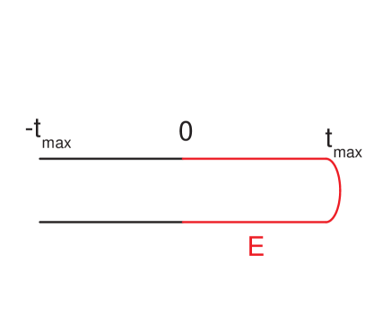
Figure 1: Kadanoff-Baym-Keldysh time contour for the two-time contour-ordered Green function in nonequilibrium. The red line corresponds to the region of time where the electric field is nonzero ($t>0$).

The indices $H$ and $I$ on the right hand side of Eq. (III) stand for the Heisenberg and Interaction representations for the electron operators. $H(-t_{\rm max})$ corresponds to the Hamiltonian in the case of zero electric field. The expression in Eq. (III) is a formal generalization of the equilibrium formulas to the nonequilibrium case. Therefore, all the machinery of equilibrium quantum many-body theory, including Wick’s theorem and the different relations between the Green functions, the self-energies and the vertex functions can be directly applied to the nonequilibrium case as long as we replace time-ordered objects by the contour-ordered objects along the contour of Fig. 1 (see, for example, Ref. Rammer, for an appropriate discussion).

In this work, we use the two-branch Keldysh contour, which is appropriate when we directly solve the problem on the lattice (rather than using DMFT techniques, where the contour is necessarily more complicated). This contour consists of two horizontal branches: one runs to the right and the other to the left. Such a time contour is needed to be able to calculate both time-ordered and so-called lesser or greater Green functions, because it allows us to use time ordering along the whole contour to determine those objects. Because of the time ordering, we can use Wick’s theorem to evaluate different correlation functions for the perturbative expansion. In general, there are four different Green functions one defines by taking the time coordinates along the upper $+$ or lower $-$ branch. These are the time-ordered, lesser, greater, and anti-time-ordered Green functions. They satisfy

$$G^{T}_{\bf k}(t_{1},t_{2}) = G^{c}_{\bf k}(t_{1}^{+},t_{2}^{+})$$ (12)

$$= -i\langle{\rm T}c_{{\bf k}H}(t_{1})c^{\dagger}_{{\bf k}H}(t_{2})\rangle,$$

$$G^{<}_{\bf k}(t_{1},t_{2}) = G^{c}_{\bf k}(t_{1}^{+},t_{2}^{-})$$ (13)

$$= i\langle c^{\dagger}_{{\bf k}H}(t_{2})c_{{\bf k}H}(t_{1})\rangle,$$

$$G^{>}_{\bf k}(t_{1},t_{2}) = G^{c}_{\bf k}(t_{1}^{-},t_{2}^{+})$$ (14)

$$= -i\langle c_{{\bf k}H}(t_{1})c^{\dagger}_{{\bf k}H}(t_{2})\rangle,$$

$$G^{\bar{T}}_{\bf k}(t_{1},t_{2}) = G^{c}_{\bf k}(t_{1}^{-},t_{2}^{-})$$ (15)

$$= -i\langle{\rm\bar{T}}c_{{\bf k}H}(t_{1})c^{\dagger}_{{\bf k}H}(t_{2})\rangle,$$

where the $+$ and $-$ signs indicate whether the real times $t_{1}$ and $t_{2}$ lie on the upper (positive time direction) or lower (negative time direction) branch of the time contour, the symbol T is ordinary time ordering and the symbol ${\rm\bar{T}}$ is anti time ordering. The more familiar retarded and advanced Green functions satisfy

$$G^{R}_{\bf k}(t_{1},t_{2}) = G^{T}_{\bf k}(t_{1},t_{2})-G^{<}_{\bf k}(t_{1},t_{2})$$ (16)

$$= -G^{\bar{T}}_{\bf k}(t_{1},t_{2})+G^{>}_{\bf k}(t_{1},t_{2}),$$

$$G^{A}_{\bf k}(t_{1},t_{2}) = G^{T}_{\bf k}(t_{1},t_{2})-G^{>}_{\bf k}(t_{1},t_{2})$$ (17)

$$= -G^{\bar{T}}_{\bf k}(t_{1},t_{2})+G^{<}_{\bf k}(t_{1},t_{2}),$$

and the so-called Keldysh Green function is

$$G^{K}_{\bf k}(t_{1},t_{2}) = G^{<}_{\bf k}(t_{1},t_{2})+G^{>}_{\bf k}(t_{1},t_{2})$$ (18)

$$= G^{T}_{\bf k}(t_{1},t_{2})+G^{\bar{T}}_{\bf k}(t_{1},t_{2}).$$

It is sometimes convenient to introduce a two-component Fermi-field operator

$${\tilde{c}}_{{\bf k}}(t)=\left(\begin{array}[]{c}c_{{\bf k}}(t^{+})\\ c_{{\bf k}}(t^{-})\end{array}\right),\ \ \ \ {\tilde{c}}_{{\bf k}}^{\dagger}(t)=\left(c_{{\bf k}}^{\dagger}(t^{+}),c_{{\bf k}}^{\dagger}(t^{-})\right)$$ (19)

with the components also defined on the upper and lower time branches of the time contour. In this case, the following matrix Green function can be introduced:

$${\hat{G}}_{{\bf k}}^{c}(t_{1},t_{2})=\left(\begin{array}[]{cc}G_{{\bf k}}(t_{1}^{+},t_{2}^{+})\\ G_{{\bf k}}(t_{1}^{-},t_{2}^{+})\end{array}\begin{array}[]{cc}G_{{\bf k}}(t_{1}^{+},t_{2}^{-})\\ G_{{\bf k}}(t_{1}^{-},t_{2}^{-}).\end{array}\right)$$ (20)

In order to transform the matrix in Eq. (20) to a form more convenient for computation and often used to study nonequilibrium problems, we make the combined Keldysh and Larkin-Ovchinnikov (LO) transformation Larkin ; Rammer :

$${\hat{G}}_{{\bf k}}^{T}(t_{1},t_{2})\rightarrow{\hat{L}}{\hat{\tau}}_{z}{\hat{G}}_{{\bf k}}^{T}(t_{1},t_{2}){\hat{L}}^{\dagger},$$ (21)

where ${\hat{L}}=(1/\sqrt{2})({\hat{\tau}}_{0}-i{\hat{\tau}}_{y})$, and ${\hat{\tau}}_{i},i=0,x,y,z$, are the Pauli matrices. Under such a transformation, the Green function in Eq. (20) acquires the following form:

$${\hat{G}}_{{\bf k}}^{c}(t_{1},t_{2})=\left(\begin{array}[]{c}G_{{\bf k}}^{R}(t_{1},t_{2})\\ 0\end{array}\begin{array}[]{c}G_{{\bf k}}^{K}(t_{1},t_{2})\\ G_{{\bf k}}^{A}(t_{1},t_{2})\end{array}\right),$$ (22)

where the retarded, advanced and the Keldysh Green functions are also expressed as

$$G_{\bf k}^{R}(t_{1},t_{2})=-i\theta(t_{1}-t_{2})\left\langle\left\{c_{{\bf k}H}(t_{1}),c_{{\bf k}H}^{\dagger}(t_{2})\right\}\right\rangle,$$ (23)

$$G_{\bf k}^{A}(t_{1},t_{2})=i\theta(t_{2}-t_{1})\left\langle\left\{c_{{\bf k}H}(t_{1}),c_{{\bf k}H}^{\dagger}(t_{2})\right\}\right\rangle,$$ (24)

$$G_{\bf k}^{K}(t_{1},t_{2})=-i\left\langle\left[c_{{\bf k}H}(t_{1}),c_{{\bf k}H}^{\dagger}(t_{2})\right]\right\rangle.$$ (25)

The square (curly) brackets correspond to the commutator (anti-commutator). In this representation, the time arguments of Green functions (23)-(25) are real times.

In the nonequilibrium case, all the information about the properties of a system is contained in two basic electron Green functions. The most often used ones are the retarded function in Eq. (23) and the lesser function in Eq. (13).

The retarded Green function contains information about the spectra of the system, and the lesser Green function describes the occupation of these states. These two functions form an independent Green function basis, and any other Green function can be expressed by means of these two functions; in the equilibrium case, only one Green function is independent (since the states are distributed according to the Fermi-Dirac distribution). In particular, it is easy to find a useful relation, which follows from the definitions in Eqs. (23), (24), (25) and (13):

$$G_{\bf k}^{<}(t_{1},t_{2})=\frac{1}{2}\left(G_{\bf k}^{K}(t_{1},t_{2})-G_{\bf k}^{R}(t_{1},t_{2})+G_{\bf k}^{A}(t_{1},t_{2})\right).$$ (26)

The self-energy representation, which corresponds to Eq. (22) has the same form:

$${\hat{\Sigma}}_{{\bf k}}^{c}(t_{1},t_{2})=\left(\begin{array}[]{c}\Sigma^{R}_{{\bf k}}(t_{1},t_{2})\\ 0\end{array}\begin{array}[]{c}\Sigma^{K}_{{\bf k}}(t_{1},t_{2})\\ \Sigma^{A}_{{\bf k}}(t_{1},t_{2})\end{array}\right).$$ (27)

In this representation one can also apply the standard Wick rules to evaluate the different operator averages of the perturbative expansion. In fact, it is possible to show that the nonequilibrium and equilibrium field theories are formally equivalent if one introduces the time ordering along the contour instead of the usual “equilibrium” time orderingLangreth .

The Dyson equation which connects the contour-ordered Green function in Eq. (22) and self-energy, remains valid:

$${\hat{G}}_{{\bf k}}^{c}(t_{1},t_{2})={\hat{G}}_{{\bf k}}^{0c}(t_{1},t_{2})+\left[{\hat{G}}_{{\bf k}}^{0c}{\hat{\Sigma}}_{{\bf k}}^{c}{\hat{G}}_{{\bf k}}^{c}\right](t_{1},t_{2}),$$ (28)

where ${\hat{G}}_{{\bf k}}^{0c}(t_{1},t_{2})$ is the nonequilibrium Green function in the case of no interactions, and the product of the three operators in the last term is a shorthand notation for an implicit matrix multiplication of the continuous matrix operators over their respective internal time coordinates (evaluated along the contour). Its components can be found analytically. For the conduction electrons, we have

$$G_{{\bf k}}^{R0}(t_{1},t_{2}) = -i\theta(t_{1}-t_{2})\exp[i\mu^{(0)}(t_{1}-t_{2})]$$ (29)

$$\times \exp\left[-i\int_{t_{2}}^{t_{1}}d{\bar{t}}\epsilon\left({\bf k}-e{\bf A}({\bar{t}})\right)\right],$$

$$G_{{\bf k}}^{A0}(t_{1},t_{2}) = i\theta(t_{2}-t_{1})\exp[i\mu^{(0)}(t_{1}-t_{2})]$$ (30)

$$\times \exp\left[-i\int_{t_{2}}^{t_{1}}d{\bar{t}}\epsilon\left({\bf k}-e{\bf A}({\bar{t}})\right)\right],$$

$$G_{{\bf k}}^{K0}(t_{1},t_{2}) = i\{2f[\epsilon({\bf k})-\mu^{(0)}]-\}1\exp[i\mu^{(0)}(t_{1}-t_{2})]$$ (31)

$$\times \exp\left[-i\int_{t_{2}}^{t_{1}}d{\bar{t}}\epsilon\left({\bf k}-e{\bf A}({\bar{t}})\right)\right],$$

where $f[\epsilon({\bf k})-\mu^{(0)}]=1/\{1+\exp[\beta\{\epsilon({\bf k})-\mu^{(0)}\}]\}$ is the Fermi-Dirac distribution function for free electrons. The symbol $\mu^{(0)}$ is the noninteracting chemical potential. While the $f$-electron Green functions are:

$$F_{{\bf k}}^{R0}(t_{1},t_{2})=-i\theta(t_{1}-t_{2})e^{i\mu_{f}^{(0)}(t_{1}-t_{2})},$$ (32)

$$F_{{\bf k}}^{A0}(t_{1},t_{2})=i\theta(t_{2}-t_{1})e^{i\mu_{f}^{(0)}(t_{1}-t_{2})},$$ (33)

$$F_{{\bf k}}^{K0}(t_{1},t_{2})=i(2n_{f}-1)e^{i\mu_{f}^{(0)}(t_{1}-t_{2})}.$$ (34)

Here, $\mu_{f}^{(0)}$ is the noninteracting chemical potential for the $f$-electrons and $n_{f}$ is the concentration of $f$-electrons. As expected, the free $f$-electron Green functions are momentum-independent. Note that at half-filling, we have $\mu^{(0)}=\mu_{f}^{(0)}=0$ and $n_{f}=1/2$, so that the noninteracting Green functions simplify, and in particular $F_{{\bf k}}^{K0}=0$.

The Dyson equation in Eq. (28) is equivalent to the following system of three equations:

$$G_{\bf k}^{R}(t_{1},t_{2})=G_{\bf k}^{R0}(t_{1},t_{2})+[G_{\bf k}^{R0}\Sigma_{{\bf k}}^{R}G_{\bf k}^{R}](t_{1},t_{2}),$$ (35)

$$G_{\bf k}^{A}(t_{1},t_{2})=G_{\bf k}^{A0}(t_{1},t_{2})+[G_{\bf k}^{A0}\Sigma_{{\bf k}}^{A}G_{\bf k}^{A}](t_{1},t_{2}),$$ (36)

$$G_{\bf k}^{K}(t_{1},t_{2}) = [1+G_{\bf k}^{R}\Sigma_{{\bf k}}^{R}]G_{\bf k}^{K0}[1+\Sigma_{\bf k}^{A}G_{\bf k}^{A}](t_{1},t_{2})$$ (37)

$$+ [G_{\bf k}^{R}\Sigma_{{\bf k}}^{K}G_{\bf k}^{A}](t_{1},t_{2}).$$

This is derived by simply writing down the Dyson equation for every matrix component. The 21 component is trivial, since every 21 matrix component is equal to zero. We omit the internal time integrals (over the real-time axis) in Eqs. (35)-(37) for sake of brevity.

In general, it is difficult to solve this system of equations, especially in the nonequilibrium case when electron interactions are present. However, for the Falicov-Kimball model the electron self-energy is momentum-independent through second order in the interaction $U$, which simplifies the analysis. In the next Section, we shall present the perturbative solution of Eq. (28), or equivalently Eqs. (35)-(37), for the Green function.

IV Perturbation theory

We will investigate a non-self-consistent perturbative expansion that is strictly truncated to second order in $U$. We perform the expansion directly for the lattice Hamiltonian, which is worked out (for the equilibrium case) in the Appendix. As mentioned above, the first and second-order self-energies are local because the $f$-electron Green function is local in all dimensions. The expression for the nonequilibrium self-energy can be obtained from the corresponding expression for the equilibrium time-ordered self-energy by making the Langreth substitutionLangreth for the corresponding Green functions, which tells us to replace all integrals over the real time axis by integrals over the contour, and to replace all time-ordered objects by contour-ordered objects. The equilibrium time-ordered self-energy has the following expression when strictly truncated to second order in $U$ (see Appendix A)

$$\Sigma_{lm}(t_{1},t_{2}) = \delta_{lm}[\delta(t_{1}-t_{2})(Un_{f}-\mu+\mu^{(0)})$$ (38)

$$+ U^{2}G_{ll}^{0}(t_{1},t_{2})F_{ll}^{0}(t_{2},t_{1})F_{ll}^{0}(t_{1},t_{2})]$$

where $l$ and $m$ denote lattice sites and we have suppressed the time-ordered superscript on all quantities. Using the fact that the product of the $f$-electron Green functions is $n_{f}(1-n_{f})$, yields the final expression for the second-order equilibrium self-energy

$$\Sigma_{lm}^{(2)}(t_{1},t_{2})=\delta_{lm}U^{2}n_{f}(1-n_{f})G_{ll}^{0}(t_{1},t_{2}).$$ (39)

Note that this expression cannot immediately be used to find the equilibrium retarded self-energy. In order to find that, we can determine the time-ordered self-energy on the imaginary time axis, Fourier transform to Matsubara frequencies and then perform an analytic continuation to the real axis to find the retarded self-energy. An alternate method, which we will adopt here, is to find the equilibrium lesser self-energy from the nonequilibrium formalism (evaluated in the equilibrium limit). Then the equilibrium retarded self-energy follows by taking the difference of the equilibrium time-ordered and lesser self-energies.

In the nonequilibrium case, we use the Langreth ruleLangreth to replace the integrals over real time by integrals over the contour. Then by examining time arguments on each of the two branches, and following the same strategy as in the appendix, we find

$$\Sigma^{T(2)}(t_{1},t_{2}) = U^{2}G^{T0}(t_{1},t_{2})F^{T0}(t_{1},t_{2})F^{T0}(t_{2},t_{1})$$ (40)

$$\Sigma^{<(2)}(t_{1},t_{2}) = U^{2}G^{<0}(t_{1},t_{2})F^{<0}(t_{1},t_{2})F^{>0}(t_{2},t_{1})$$ (41)

$$\Sigma^{>(2)}(t_{1},t_{2}) = U^{2}G^{>0}(t_{1},t_{2})F^{>0}(t_{1},t_{2})F^{<0}(t_{2},t_{1})$$ (42)

$$\Sigma^{\bar{T}(2)}(t_{1},t_{2}) = U^{2}G^{\bar{T}0}(t_{1},t_{2})F^{\bar{T}0}(t_{1},t_{2})F^{\bar{T}0}(t_{2},t_{1}).$$ (43)

Each pair of products of $f$-electron Green functions is equal to $n_{f}(1-n_{f})$, so after performing the Keldysh and the LO transformations, we get

$$\left(\begin{array}[]{c}\Sigma^{R(2)}\\ 0\end{array}\begin{array}[]{c}\Sigma^{K(2)}\\ \Sigma^{A(2)}\end{array}\right)(t_{1},t_{2}) = U^{2}n_{f}(1-n_{f})$$ (48)

$$\times \left(\begin{array}[]{c}G^{R0}\\ 0\end{array}\begin{array}[]{c}G^{K0}\\ G^{A0}\end{array}\right)(t_{1},t_{2}),$$ (53)

where all the Green functions are local. For instance,

$$G^{R0}(t_{1},t_{2})=\frac{1}{N}\sum_{\bf k}G^{R0}_{{\bf k}}(t_{1},t_{2}).$$ (54)

This approach also allows us to determine the equilibrium retarded self-energy by simply evaluating the results in the absence of an electric field. This is an example of how one uses the nonequilibrium technique to complete an equilibrium analytic continuation.

Now we will focus on the half-filled case [where $n_{f}(1-n_{f})=1/4$, $\mu^{(0)}=\mu_{f}^{(0)}=0$, and the first-order self-energy vanishes]. The formal expressions for the Green functions can be found from the appropriate Dyson equations [Eqs. (35)-(37)]. Here, we write down the results only for the half-filled case:

$$G_{\bf k}^{R(2)}(t_{1},t_{2})=G_{\bf k}^{R0}(t_{1},t_{2})+[G_{\bf k}^{R0}\Sigma^{R(2)}G_{\bf k}^{R0}](t_{1},t_{2}),$$ (55)

$$G_{\bf k}^{A(2)}(t_{1},t_{2})=G_{\bf k}^{A0}(t_{1},t_{2})+[G_{\bf k}^{A0}\Sigma^{A(2)}G_{\bf k}^{A0}](t_{1},t_{2}),$$ (56)

$$G_{\bf k}^{K(2)}(t_{1},t_{2}) = G_{\bf k}^{K0}(t_{1},t_{2})+[G_{\bf k}^{R0}\Sigma^{R(2)}G_{\bf k}^{K0}$$

$$+ G_{\bf k}^{K0}\Sigma^{A(2)}G_{{\bf k}}^{A0}+G_{\bf k}^{R0}\Sigma^{K(2)}G_{\bf k}^{A0}](t_{1},t_{2}),$$

where the second-order self-energies $\Sigma^{(2)}$ and the free Green functions $G^{0}$ are given by the half-filled case in Eqs. (48) and (29)-(31), respectively. (In the general case, we need to also include the first-order self-energy and its iterated second-order contribution.)

The free $c$-electron local Green functions (in the presence of a spatially uniform electric field), which are necessary to calculate the self-energy (48), can be found by summing Eqs. (29)-(31) over momentum [as in Eq. (54)]Turkowski :

$$G^{R0}(t_{1},t_{2}) = -i\theta(t_{1}-t_{2})e^{i\mu^{(0)}(t_{1}-t_{2})}$$ (58)

$$\times \exp\left\{-\frac{1}{4}\left[\left(\int_{t_{2}}^{t_{1}}d{\bar{t}}\cos\left(e{\bf A}({\bar{t}})\right)\right)^{2}\right.\right.$$

$$+ \left.\left.\left(\int_{t_{2}}^{t_{1}}d{\bar{t}}\sin\left(e{\bf A}({\bar{t}})\right)\right)^{2}\right]\right\},$$

$$G^{A0}(t_{1},t_{2}) = i\theta(t_{2}-t_{1})e^{i\mu^{(0)}(t_{1}-t_{2})}$$ (59)

$$\times \exp\left\{-\frac{1}{4}\left[\left(\int_{t_{2}}^{t_{1}}d{\bar{t}}\cos\left(e{\bf A}({\bar{t}})\right)\right)^{2}\right.\right.$$

$$+ \left.\left.\left(\int_{t_{2}}^{t_{1}}d{\bar{t}}\sin\left(e{\bf A}({\bar{t}})\right)\right)^{2}\right]\right\},$$

$$G^{K0}(t_{1},t_{2}) = ie^{i\mu^{(0)}(t_{1}-t_{2})}$$ (60)

$$\times \exp\left\{-\frac{1}{4}\left(\int_{t_{2}}^{t_{1}}d{\bar{t}}\sin\left(e{\bf A}({\bar{t}})\right)\right)^{2}\right\}$$

$$\times\int d\epsilon\rho(\epsilon)[2f(\epsilon-\mu^{(0)})-1]$$

$$\times\exp\left\{-i\epsilon\int_{t_{2}}^{t_{1}}d{\bar{t}}\cos\left(e{\bf A}({\bar{t}})\right)\right\},$$

where

$$\rho(\epsilon)=\frac{1}{\sqrt{\pi}}e^{-\varepsilon^{2}}$$ (61)

is the free electron density of states on the hypercubic lattice in infinite dimensions (the generalization to finite dimensions is obvious). At half-filling we have $\mu^{(0)}=0$ in Eqs. (58)-(60).

Thus, we have obtained the formal expressions for the second-order nonequilibrium retarded, advanced and Keldysh Green functions (35)-(37), with the free Green functions defined by Eqs. (29)-(31), (58)-(60) and the self-energies in Eq. (48). In the following Section, we shall use these solutions to study the time-dependence of the electric current in the case when an external time-dependent electric field [Eq. (6)] is present.

Before proceeding with the nonequilibrium solutions we would like to study some of the equilibrium properties of the retarded self-energy $\Sigma$. We check the perturbative result for the self-energy in Eq. (48) versus the exact DMFT results in equilibrium and estimate the values of $U$ above which the second order equilibrium perturbation theory fails. It is natural to suppose that the second order nonequilibrium perturbation theory results are also inaccurate when $U$ is that large.

Using the results in Eq. (48), we find the expression for the second order self-energy has the following form in frequency space (at half-filling):

$$\Sigma^{R}(\omega) = \frac{U^{2}}{4}G^{R0}(\omega),$$ (62)

$$= \frac{U^{2}}{4}\left[{\rm\hat{P}}\int d\varepsilon\rho(\epsilon)\frac{1}{\omega-\varepsilon}-i\pi\rho(\omega)\right],$$

where the symbol ${\rm\hat{P}}$ denotes the principle value of the integral, and $\rho(\epsilon)$ is defined in Eq. (61). In order to estimate the values of $U$, for which the second order perturbation theory gives good results in equilibrium, we compare the imaginary part of the perturbative retarded self-energy

$${\rm Im}\Sigma^{R}(\omega)=-\frac{\sqrt{\pi}U^{2}}{4}e^{-\omega^{2}}$$ (63)

with the exact self-energy calculated by the DMFT approach. The frequency dependence of $-{\rm Im}\Sigma^{R}$ for different values of $U$ is presented in Fig. 2. As follows from this figure, the second order perturbation theory gives reasonable results up to $U\sim 0.5$. Hence, we expect that the result in Eq. (48) will also be accurate when $U<0.5$ for the nonequilibrium case.

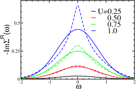
Figure 2: Frequency dependence of the imaginary part of the second order retarded self-energy for different values of the Coulomb repulsion $U$ (solid lines). The dashed lines are the corresponding exact dynamical mean-field theory results.

V The electric current

V.1 Semiclassical Boltzmann equation approximation for the current

Before analyzing the time dependence of the current in the quantum case, we present the approximation for the current that follows from a semiclassical Boltzmann equation approach. The Boltzmann equation for the nonequilibrium quasiparticle distribution function $f^{\rm non}({\bf k},t)=-iG_{{\bf k}}^{<}(t,t)$ becomes

$$\frac{\partial f^{\rm non}({\bf k},t)}{\partial t}+e{\bf E}(t)\cdot\nabla_{\bf k}f^{\rm non}({\bf k},t)=-\frac{1}{\tau}[f^{\rm non}({\bf k},t)-f({\bf k})],$$ (64)

in the case of a spatially uniform time-dependent electric field. Here, $\tau$ is the scattering time, which typically is proportional to $1/U^{2}$ in the weak correlated limit of the Falicov-Kimball model (because it is inversely proportional to the imaginary part of the self-energy at zero frequency) and the r.h.s. of the equation is the collision term. Note that in the quantum case, the quantum Boltzmann equation is more complicated because the quantum excitations depend on two independent times, not one. Hence, it isn’t obvious that we should use the quantum relaxation time in the semiclassical Boltzmann equation; indeed, we often find that by fitting to a somewhat longer relaxation time, we can improve the fit to the Boltzmann equation rather dramatically, but we present the results using a fixed relaxation time here. Of course, our numerical nonequilibrium results presented below are equivalent to exactly solving the full quantum Boltzmann equation, but our method of solution is different.

The boundary condition for the semiclassical Boltzmann equation is:

$$f^{\rm non}({\bf k},t=0) = f({\bf k})$$ (65)

$$= \frac{1}{\exp[\beta(\varepsilon({\bf k})-\mu)]+1}.$$

We will be considering only the case of half-filling, where we can set the chemical potential to zero. The solution of Eqs. (64) and (65) when the electric field is pointing in the diagonal direction ${\bf E}(t)=E(1,1,...,1)\theta(t)$ has the following form:

$$f^{\rm non}({\bf k},t)=\frac{1}{\tau}\int_{-\infty}^{t}d{\bar{t}}e^{-(t-{\bar{t}})/\tau}f\left({\bf k}+e\int_{t}^{{\bar{t}}}dt^{\prime}{\bf E}(t^{\prime})\right).$$ (66)

The total current can now be determined from the distribution function

$$j(t)=-\frac{e}{\tau}\sum_{{\bf k}}{\bar{\varepsilon}}({\bf k})\int_{-\infty}^{t}d{\bar{t}}e^{-(t-{\bar{t}})/\tau}f\left({\bf k}+e\int_{t}^{{\bar{t}}}dt^{\prime}{\bf E}(t^{\prime})\right).$$ (67)

Shifting the momentum via ${\bf k}\rightarrow{\bf k}-e\int_{t}^{{\bar{t}}}dt^{\prime}{\bf E}(t^{\prime})$ and then integrating over the Brillouin zone gives the following analytical expression for the current:

$$j(t) = -\frac{e}{\sqrt{d}}\frac{eE\tau}{1+e^{2}E^{2}\tau^{2}}\int d\varepsilon\rho(\varepsilon)\varepsilon f(\varepsilon)$$ (68)

$$\times \left[1-\left(\cos(eEt)-eE\tau\sin(eEt)\right)e^{-t/\tau}\right].$$

Analysis of this solution shows that the current is a strongly oscillating function of time for $t\ll\tau$ (when $E$ is large) which then approaches the steady-state value

$$j^{\rm steady}=\frac{eE\tau}{1+e^{2}E^{2}\tau^{2}}j_{0},$$ (69)

where

$$j_{0}=-\frac{e}{\sqrt{d}}\int d\varepsilon\rho(\varepsilon)\varepsilon f(\varepsilon),$$ (70)

for $t\gg\tau$ (see Fig. 3 for an example of the solutions in the infinite-dimensional limit). It is interesting that the amplitude of the steady-state current is proportional to $E$ in the case of a weak field (the linear-response regime), and then becomes proportional to $1/E$ when the field is strong ($eE\gg 1/\tau$). In this nonlinear regime, the amplitude of the current goes to zero as the field increases. As it will be shown in the following Subsection, the exact quantum solution of the problem results in qualitatively different behavior from the Boltzmann case for the current as a function of time.

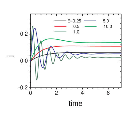
Figure 3: Boltzmann equation solution for the time-dependence of the electric current for different values of the electric field in the limit of infinite dimensions at $\tau=1,\beta=10$. Here and in Figs. 4–7, we set the prefactor $e/\sqrt{d}$ in the results for the electric current [see Eqs. (68) and (77)] to be equal to $1$.

V.2 Perturbative expansion for the current in the quantum case

In the quantum case, the electrical current can be found by calculating the expectation value of the electrical current operator. This operator is formed from the sum over momentum of the product of the electric charge times the velocity vector at k times the number operator for electrons in state k. Hence, the time-dependence of the expectation value of the electric current components is

$$j_{\alpha}(t)=e\sum_{{\bf k}}\frac{\partial}{\partial k_{\alpha}}\epsilon\left({\bf k}-e{\bf A}(t)\right)\langle c_{{\bf k}}^{\dagger}(t)c_{{\bf k}}(t)\rangle,$$ (71)

which becomes

$$j_{\alpha}(t)=-i\frac{e}{\sqrt{d}}\sum_{{\bf k}}\sin\left(k_{\alpha}-eA_{\alpha}(t)\right)G_{{\bf k}}^{<}(t,t),$$ (72)

after using the definition of the lesser Green function. This Green function can be found from Eq. (26), where the expressions for the retarded, advanced and Keldysh Green functions on the r.h.s. of Eq. (26) are given by Eqs. (55)-(IV). Since the electric field lies along the lattice diagonal, all its components are equal to each other, and the magnitude of the electric current becomes:

$$j(t)=\sqrt{d}j_{\alpha}(t),$$ (73)

for any component $\alpha$ The momentum summation in Eq. (72) can be performed by using the definitions of energy functions in Eqs. (8) and (9) and the expression for joint density of states in Eq. (10):

$$j(t) = \frac{ie}{2\sqrt{d}}\int d\epsilon\int d{\bar{\epsilon}}\rho_{2}(\epsilon,{\bar{\epsilon}})$$ (74)

$$\times \left[{\bar{\epsilon}}\cos\left(eA_{\alpha}(t)\right)-\epsilon\sin\left(eA_{\alpha}(t)\right)\right]$$

$$\times\left[G_{\epsilon,{\bar{\epsilon}}}^{K}(t,t)-G_{\epsilon,{\bar{\epsilon}}}^{R}(t,t)+G_{\epsilon,{\bar{\epsilon}}}^{A}(t,t)\right].$$

The sum of the last two terms in Eq. (74) gives zero, since

$$-G_{\epsilon,{\bar{\epsilon}}}^{R}(t_{1},t_{2})+G_{\epsilon,{\bar{\epsilon}}}^{A}(t_{1},t_{2}) = i\langle\{c_{{\bf k}}(t_{1}),c_{{\bf k}}^{\dagger}(t_{2})\}\rangle$$ (75)

$$= i\delta(t_{1}-t_{2})$$

is momentum-independent and the velocity is an odd function of momentum.

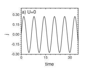
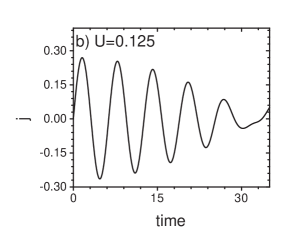
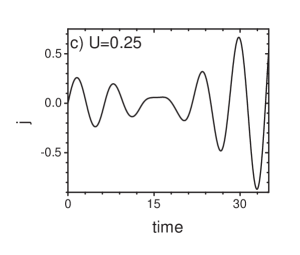
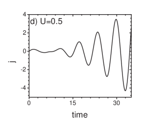
Figure 4: The PT electric current as a function of time for $E=1,\beta=10$ and different values of $U$. Note the unphysical increase in the current at long times.

Therefore,

$$j(t) = \frac{ie}{2\sqrt{d}}\int d\epsilon\int d{\bar{\epsilon}}\rho_{2}(\epsilon,{\bar{\epsilon}})\left[{\bar{\epsilon}}\cos\left(eA_{\alpha}(t)\right)\right.$$

$$- \left.\epsilon\sin\left(eA_{\alpha}(t)\right)\right]\left[G_{\epsilon,{\bar{\epsilon}}}^{K0}(t,t)\right.$$

$$+ \frac{U^{2}}{4}\int_{-\infty}^{+\infty}dt_{1}\int_{-\infty}^{+\infty}dt_{2}$$

$$\times (G_{\epsilon,{\bar{\epsilon}}}^{R0}(t,t_{1})G_{loc}^{R0}(t_{1},t_{2})G_{\epsilon,{\bar{\epsilon}}}^{K0}(t_{2},t)$$

$$+ \left.G_{\epsilon,{\bar{\epsilon}}}^{K0}(t,t_{1})G_{loc}^{A0}(t_{1},t_{2})G_{\epsilon,{\bar{\epsilon}}}^{A0}(t_{2},t)\right.$$

$$+ \left.G_{\epsilon,{\bar{\epsilon}}}^{R0}(t,t_{1})G_{loc}^{K0}(t_{1},t_{2})G_{\epsilon,{\bar{\epsilon}}}^{A0}(t_{2},t))\right],$$

where we restricted to the half-filling case, used Eq. (48), and neglected the term that is fourth order in $U$. Integration over ${\bar{\varepsilon}}$ in Eq. (74) yields

$$j(t) = \frac{e}{\sqrt{d}}\int d\varepsilon\rho(\varepsilon)\varepsilon f(\varepsilon)\sin(eA(t))$$ (77)

$$+ \frac{eU^{2}}{4\sqrt{d}}\int_{-\infty}^{t}dt_{1}\int_{-\infty}^{t_{1}}dt_{2}\left[-\frac{i}{2}S(t_{2},t_{1})\cos(eA(t))\right.$$

$$- \varepsilon\sin(eA(t))\Big{]}\exp\left[-\frac{1}{4}\left\{C^{2}(t_{2},t_{1})+2S^{2}(t_{2},t_{1})\right\}\right]$$

$$\times \int d\varepsilon\rho(\varepsilon)[2f(\varepsilon)-1]\exp[-i\varepsilon C(t_{2},t_{1})]$$

$$+ \frac{ieU^{2}}{16\sqrt{d}}\int_{-\infty}^{t}dt_{1}\int_{-\infty}^{t}dt_{2}\left[S(t_{2},t_{1})\cos(eA(t))\right.$$

$$- C(t_{2},t_{1})\sin(eA(t))\Big{]}$$

$$\times \exp\left[-\frac{1}{4}\left\{C^{2}(t_{2},t_{1})+2S^{2}(t_{2},t_{1})\right\}\right]$$

$$\times \int d\varepsilon\rho(\varepsilon)[2f(\varepsilon)-1]\exp[i\varepsilon C(t_{2},t_{1})]$$

In order to simplify the expression, we have introduced the functions

$$C(t_{2},t_{1})=\int_{t_{1}}^{t_{2}}d{\bar{t}}\cos(eA({\bar{t}}))$$

$$S(t_{2},t_{1})=\int_{t_{1}}^{t_{2}}d{\bar{t}}\sin(eA({\bar{t}})).$$ (78)

In our numerical work, we consider the current in the case of a constant electric field $E$ turned on at time $t=0$, i.e. $A(t)=-Et\theta(t)$. In this case, we find:

$$C(t_{2},t_{1}) = \theta(-t_{1})\theta(-t_{2})\left[t_{2}-t_{1}\right]$$ (79)

$$+ \theta(-t_{1})\theta(t_{2})\left[\frac{\sin(eEt_{2})}{eE}-t_{1}\right]$$

$$+ \theta(t_{1})\theta(-t_{2})\left[t_{2}-\frac{\sin(eEt_{1})}{eE}\right]$$

$$+ \theta(t_{1})\theta(t_{2})\frac{1}{eE}\left[\sin(eEt_{2})-\sin(eEt_{1})\right],$$

$$S(t_{2},t_{1}) = -\theta(-t_{1})\theta(t_{2})\frac{1}{eE}\left[1-\cos(eEt_{2})\right]$$ (80)

$$- \theta(t_{1})\theta(-t_{2})\frac{1}{eE}\left[\cos(eEt_{1})-1\right]$$

$$- \theta(t_{1})\theta(t_{2})\frac{1}{eE}\left[\cos(eEt_{1})-\cos(eEt_{2})\right].$$

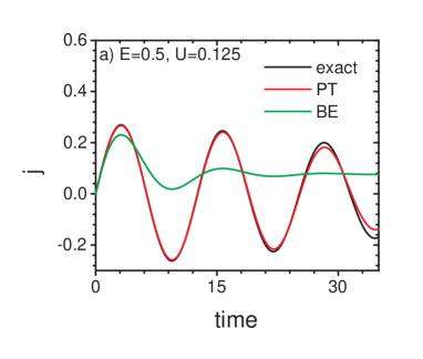
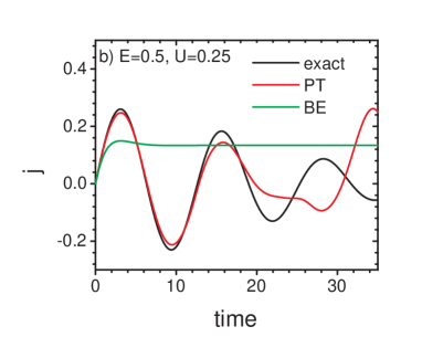
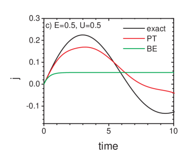
Figure 5: The PT electric current as a function of time for $E=0.5,\beta=10$ and different values of $U$ (red lines). The exact DMFT calculation results and the Boltzmann equation solution are presented by black and green lines, respectively.

Equations (77), (79) and (80) determine the time dependence of the current when a constant electric field is turned on at time $t=0$. It is difficult to find an analytic expression for $j(t)$, except for the simplest case of $U=0$. In this case:

$$j(t)=j_{0}\sin\left(eEt\right)$$ (81)

(the so-called Bloch oscillationBloch ), where the amplitude of the oscillations $j_{0}$ is given by Eq. (70) and the Bloch frequency isTurkowski $\omega_{B}=eE$. In the limit of infinite dimensions, the current amplitude $j_{0}$ can also be written as:

$$j_{0}=\frac{1}{2}\frac{e}{\sqrt{d}}\int d\epsilon\rho(\epsilon)\frac{df(\epsilon)}{d\varepsilon},$$ (82)

after integrating by parts.

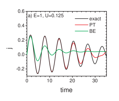
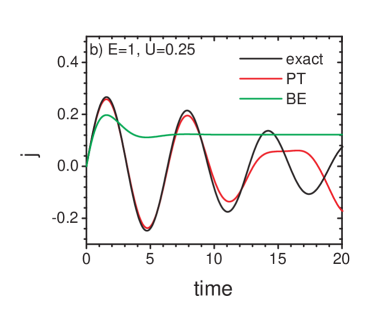
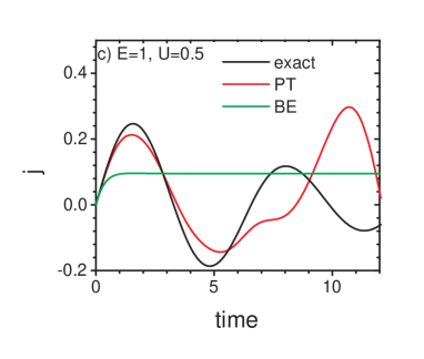
Figure 6: The PT electric current as a function of time for $E=1.0,\beta=10$ and different values of $U$ (red lines). The exact DMFT results and the Boltzmann equation solution are presented by black and green lines, respectively.

Comparison of this result with the general expression for the current given in Eq. (77) yields the following formal expression for the current in a strictly truncated perturbation theory expansion:

$$j(t)=j_{0}\sin\left(eEt\right)+U^{2}j_{2}(t).$$ (83)

Thus, the electric current is a superposition of an oscillating part and some other part, whose time-dependence will be determined below.

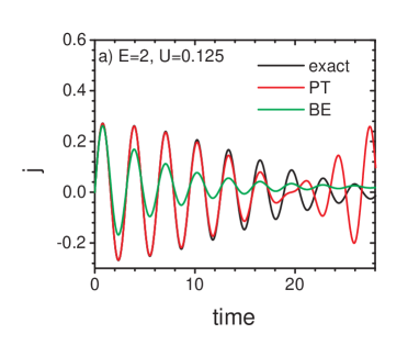
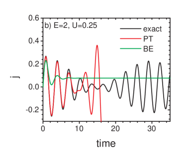
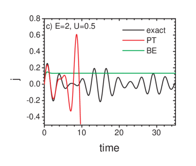
Figure 7: The PT electric current as a function of time for $E=2.0,\beta=10$ and different values of $U$ (red lines). The exact DMFT calculation results and the Boltzmann equation solution are presented by black and green lines, respectively. Note that the perturbative values for the current become so large that they are not shown for larger times.

Numerical results for the time-dependence of the electric current calculated from Eq. (77) are presented in Figs. 4–7. As follows from these figures, the current oscillates for all time. This is the main difference from the Boltzmann equation result (Fig. 3), where the current rapidly reaches a constant steady-state value. As it will be shown below, the second order perturbation theory cannot describe the steady-state regime correctly. However, the perturbation theory should give reasonable results for times smaller than $\sim 2/U$, which we consider below. As depicted in Figure 4, the current depends only weakly on $U$, except for the case $U\sim 0.5$. This is because the current is dominated by the Bloch term $j_{0}$ [see Eq. (83)]. As time increases, the amplitude of the oscillations decrease. This decrease is proportional to $U^{2}$, in agreement with Eq. (77). As $t$ increases further, the current amplitude goes through zero (at a time we call $t_{\rm pert}$), and then starts to increase dramatically. This is an unphysical result, so we assume that the perturbation theory is not valid for times larger than $t_{\rm pert}$, i.e. the time when the perturbation theory breaks down. This time is always smaller than the time needed to see the steady state develop, so this perturbation theory is not capable of producing the steady-state response. The period of the oscillations remains essentially equal to the Bloch oscillation period, but it is not well defined for damped oscillations.

The validity of the second-order nonequilibrium perturbation theory can also be checked by comparing the results for the current with exact numerical results calculated by the nonequilibrium DMFT method Nashville ; Turkowski1 ; dmft_fk . We present the corresponding results for cases of different values of $U$ and $E$ in Figs. 5–7. As shown in these Figures, the perturbation theory results are close to the exact results only for times smaller than $\sim 2/U$. Note that although the perturbation theory does show an increase in the current for intermediate times, it does not properly show the quantum beats in the current, which occur, with a beat period on the order of $1/U$, even though the shape of the curve is qualitatively similar. These beats occur only for large fields ($E\geq 2$ here).

In Figures 5–7, we also present the results for the current in the case of the Boltzmann equation solution Eq. (68), where the scattering time is fixed at the quantum Boltzmann equation value $\tau=\rho(\mu)/(4\pi|{\rm Im}\Sigma(\omega=0)|)$ (see, for example Ref. Kiel, ; this result is the transport relaxation time). Substitution of Eq. (63) into this expression yields:

$$\tau=1/(\pi^{2}U^{2}).$$ (84)

The Boltzmann equation approach shows a rapid approach to the steady state, much faster than what is seen in the exact numerical results or in the perturbation theory. Although the Boltzmann equation is accurate at small times, it is clear that the quantum system has much richer behavior than what is predicted by the semiclassical approach, at least in cases where the electric field is large. Note that the functional form of the semiclassical Boltzmann equation can fit the exact results for the current much better if we adjust the relaxation time $\tau$ to yield the best fit of the data rather than use Eq. (84), but the relaxation time then becomes just a fitting parameter and is not derived from a microscopic model.

To complete the analysis of the time-dependence of the electric current, we present an analytical expression for the electric current in the limit of strong electric fields $E\rightarrow\infty$. Substitution of Eqs. (79) and (80) into Eq. (77) gives the following result for the electric current in the limit of large electric fields:

$$j(t)\simeq - \frac{e}{\sqrt{d}}\int d\varepsilon\rho(\varepsilon)\varepsilon f(\varepsilon)$$

$$\times \left[1-U^{2}B(\beta)-\frac{U^{2}}{4}t^{2}\right]\sin(eEt),$$

where

$$B(\beta)=\left[\int d\varepsilon\rho(\varepsilon)\varepsilon f(\varepsilon)\right]^{-1}\int_{0}^{\infty}dx\int_{x}^{\infty}dyye^{-y^{2}}$$

$$\times\int d\varepsilon\rho(\varepsilon)f(\varepsilon)\sin(2\varepsilon y).$$ (86)

Numerical calculations show that this is a positive decreasing function of temperature: $0.25<B(\beta)<0.5$. As follows from Eq. (LABEL:jstrongfields), the electron-electron correlations lead to a decrease of the current amplitude at short times, since the terms proportional to $U^{2}$ in the square brackets in Eq. (LABEL:jstrongfields) have a minus sign in front of it. This correction is not large at short times, since we consider the case $U\ll 1$. However, from the numerical calculations, we find that the term in Eq. (LABEL:jstrongfields) which is proportional to $U^{2}t^{2}/4$, is dominant in the case of longer times. In fact, the current is an oscillating function of time. The oscillation amplitude, decreases with time as $1-U^{2}B(\beta)-U^{2}t^{2}/4$. At the time $t_{\rm pert}=(2/U)\sqrt{1-U^{2}B(\beta)}\simeq 2/U$ the sign in front of the amplitude changes, and the current oscillates out of phase with the $U=0$ case. It is important that the period of the oscillations is equal to the period of the Bloch oscillations in the noninteracting case. At longer times, the term proportional to $t^{2}$ is the most important and the time dependence is $j(t)\sim t^{2}\sin(eEt)$ at times longer than $\sim 2/U$. These results are in a qualitative agreement with the numerical results for the perturbation theory presented in Figs. 4–7. However, it is plain to see that the a growing amplitude for the current as time increases for $t>2/U$ is an unphysical result.

Unfortunately, it is impossible to find an analytical expression for the current in the limits of intermediate and small fields. However, our numerical analysis shows that the current qualitatively has the dependence given in Eq. (LABEL:jstrongfields). In particular, the steady state is never reached before the perturbation theory develops pathological behavior.

VI Local density of states

The time-dependent density of states can be calculated from the local retarded Green function in the following way:

$$A(\omega,T)=-\frac{1}{\pi}{\rm Im}G^{R}(\omega,T),$$ (87)

where $G^{R}(\omega,T)$ is the Fourier transform of the retarded Green function $G^{R}(t_{1},t_{2})$ with respect to the relative time coordinate $\tau=t_{1}-t_{2}$, and $T$ is the average time coordinate $T=(t_{1}+t_{2})/2$. The perturbation theory retarded Green function is determined in Eq. (55). Integration over the Brillouin zone and substitution into Eq. (87) yields:

$$A(\omega,T) = \frac{1}{\pi}\int_{0}^{\infty}d\tau\cos(\omega\tau)$$ (88)

$$\times \exp\left[-\frac{1}{4}\left(C^{2}(T+\tau/2,T-\tau/2)\right.\right.$$

$$+ \left.S^{2}(T+\tau/,T-\tau/2)\right)\Bigr{]}$$

$$\times \Bigr{\{}1-\frac{U^{2}}{4}\int_{T-\tau/2}^{T+\tau/2}dt_{3}\int_{T-\tau/2}^{t_{3}}dt_{4}$$

$$\times \exp\left[-\frac{1}{2}\left(C^{2}(t_{3},t_{4})+S^{2}(t_{3},t_{4})\right)\right]$$

$$\times \exp\left[\frac{1}{2}\left(C(T+\tau/2,T-\tau/2)C(t_{3},t_{4})\right.\right.$$

$$+ \left.S(T+\tau/2,T-\tau/2)S(t_{3},t_{4})\right)\Bigr{]}\Bigr{\}},$$

where $C(t_{3},t_{4})$ and $S(t_{3},t_{4})$ are defined in Eqs. (79) and (80).

Numerical calculations of the time dependence of the density of states show that the PT correction is small for times less than $t_{\rm pert}$ $\sim 2/U$. Similar to the caseTurkowski $U=0$, the density of states develops peaks at the Bloch frequencies. These peaks grow as time increases, essentially due to the zeroth-order DOS. However, these peaks do not split into two peaks as time increases for times less than $\sim 2/U$, except for the zero frequency peak. This result is different from the exact DMFT calculationsTurkowski1 at $U=0.5$. Generically, one expects the DOS to broaden as scattering is added, and to split, by an energy of the order of $U$ in the steady state due to the interactions; the numerical calculations indicate that this is indeed what actually happens even though the truncated perturbation theory does not explicitly show it.

It is interesting that one can also find analytical expressions for the zeroth and the first two spectral moments, which are time independent (the first and second-order moments are written for the half-filling case):

$$\int d\omega A(\omega,t)=1,$$

$$\int d\omega\omega A(\omega,t)=0,$$

$$\int d\omega\omega^{2}A(\omega,t)=\frac{1}{2}+\frac{U^{2}}{4}.$$ (89)

These results coincide with the exact results obtained in Ref. Turkowski1, at half-filling.

VII Conclusions

We have studied the response of the conduction electrons in the spinless Falicov-Kimball model to an external electric field by using a strictly truncated perturbative expansion to second order in $U$. We derived explicit expressions for the retarded, advanced and Keldysh Green functions and used them to calculate the time-dependence of the electric current and the density of states. We examined the case when a constant electric field is turned on at a particular moment of time. We found that Bloch oscillations of the current are present up to times at least as long as $t\sim 2/U$, but with a decreasing amplitude. In the perturbative approach, the oscillations are around a zero average current and the PT breaks down for longer times, so we cannot reach the steady state. This result is different from that of the semiclassical Boltzmann equation approach. There, the Bloch oscillations rapidly decay with time and the system approaches the steady state with $j={\rm const.}$ as time goes to infinity. Increasing the Coulomb repulsion reduces the amplitude of the oscillations more rapidly. The perturbation theory and the Boltzmann equation results for the electric current are close for short times.

The perturbation theory results for the Green functions can be used to test the accuracy of the numerical nonequilibrium DMFT calculations Nashville ; Turkowski1 ; dmft_fk in the case of weak correlations, when the system is not in the insulating regime. We also found excellent agreement for short times, but the PT becomes ill behaved at long times.

Our results can be generalized to more complicated cases. In particular, cases with different time-dependence for the field (pulses, periodic fields etc.) can be considered. Also higher order terms can be taken into account in the PT, or one can make the PT self-consistent. Finally, we can examine other strongly correlated models as well, where we expect similar behavior.

The most important result of this work is that it shows how difficult it is to accurately determine the steady-state response in a perturbative approach. At the very least, one needs to perform a self-consistent perturbation theory to be able to properly determine the long-time behavior, but, since we know that equilibrium PT is most inaccurate at low frequencies, it is natural to conclude that nonequilibrium PT is most inaccurate at long times. Hence, our work shows explicitly how challenging it is to try to determine the steady states of quantum systems unless one can formulate a steady-state theory from the start. Work along those lines is in progress for the exact solution via DMFT.

Appendix A Expansion for the time-ordered equilibrium self-energy to second order in U

The time-ordered self-energy $\Sigma_{lm}(t_{1},t_{2})$ can be expanded by examining an order-by-order solution of the Dyson equation (we suppress the $T$ superscript in these formulas)

$$G_{ij}(t,t^{\prime})=G_{ij}^{0}(t,t^{\prime})$$

$$+ \sum_{lm}\int dt_{1}\int dt_{2}G_{il}^{0}(t,t_{1})\Sigma_{lm}(t_{1},t_{2})G_{mj}(t_{2},t^{\prime}),$$

$$= G_{ij}^{0}(t,t^{\prime})$$

$$+ \sum_{lm}\int dt_{1}\int dt_{2}G_{il}^{0}(t,t_{1})\Sigma_{lm}^{(1)}(t_{1},t_{2})G^{0}_{mj}(t_{2},t^{\prime})$$

$$+ \sum_{lm}\int dt_{1}\int dt_{2}G_{il}^{0}(t,t_{1})\Sigma_{lm}^{(2)}(t_{1},t_{2})G_{mj}^{0}(t_{2},t^{\prime})$$

$$+ \sum_{lmnr}\int dt_{1}\int dt_{2}\int dt_{3}\int dt_{4}G_{il}^{0}(t,t_{1})$$

$$\times \Sigma_{lm}^{(1)}(t_{1},t_{2})G_{mn}^{0}(t_{2},t_{3})\Sigma^{(1)}_{nr}(t_{3},t_{4})G_{rj}^{0}(t_{4},t^{\prime}),$$ (91)

where the second equation explicitly shows the systematic expansion to order $U^{2}$ in terms of the first-order $\Sigma^{(1)}$ and second-order $\Sigma^{(2)}$ perturbative self-energies. The self-energies are found by a straightforward perturbative expansion of the evolution operator, when expressed in the interaction picture:

$$iG_{ij}(t,t^{\prime}) = \sum_{\nu=0}^{\infty}\frac{(-i)^{\nu}}{\nu!}\int dt_{1}...\int dt_{\nu}$$ (92)

$$\times \langle{\hat{T}}[{\hat{H}}_{U}(t_{1})...{\hat{H}}_{U}(t_{\nu})c_{i}(t)c_{j}^{\dagger}(t^{\prime})]\rangle_{\rm con},$$

where the interacting part of the Hamiltonian is

$${\hat{H}}_{U}(t_{1}) = -[\mu-\mu^{(0)}]\sum_{i}c_{i}^{\dagger}c_{i}-[\mu_{f}-\mu_{f}^{(0)}]\sum_{i}f_{i}^{\dagger}f_{i}$$ (93)

$$+ U\sum_{i}f_{i}^{\dagger}f_{i}c_{i}^{\dagger}c_{i}$$

and the statistical average is taken with respect to the free Hamiltonian ${\hat{H}}_{0}=-\sum_{\langle ij\rangle}t_{ij}c_{i}^{\dagger}c_{j}-\mu^{(0)}\sum_{i}c_{i}^{\dagger}c_{i}-\mu_{f}^{(0)}\sum_{i}f_{i}^{\dagger}f_{i}$. The subscript “con” indicates that we take only the connected contractions generated by Wick’s theorem, which must connect the conduction electron operators for all time values in the matrix elements; the connected diagrams are included because the disconnected diagrams cancel from a similar expansion of the partition function, which appears in the denominator of the matrix-element average. We have included the terms with the shift of the chemical potentials into Eq. (93), since $(\mu-\mu^{(0)})\sim(\mu_{f}-\mu_{f}^{(0)})\sim U$. Expanding the electron Green function in Eq. (92) up to second order in the interaction and using the definition of the self-energy in Eq. (91), one finds

$$\Sigma^{(1)}_{lm}(t_{1},t_{2})=(Un_{f}-\mu+\mu^{(0)})\delta_{lm}\delta(t_{1}-t_{2}),$$ (94)

and

$$\Sigma^{(2)}_{lm}(t_{1},t_{2})=U^{2}G^{0}_{lm}(t_{1}-t_{2})F^{0}_{lm}(t_{1}-t_{2})F^{0}_{ml}(t_{2}-t_{1}),$$ (95)

which depends on the difference of the times because we are in equilibrium. Since the $f$-electron Green function is local, the second-order self-energy must have $l=m$. Furthermore, since all of the Green functions are time-ordered Green functions, the product of the two $f$-electron Green functions is equal to $n_{f}(1-n_{f})$.

References

- (1) C. H. Ahn, J.-M. Triscone and J. Mannhart, Nature 424, 1015 (2003).
- (2) B. Doyon and N. Andrei, cond-mat/0506235.
- (3) P. Mehta and N. Andrei, Phys. Rev. Lett. 96, 216802 (2006).
- (4) T. Ogasawara, M. Ashida, N. Motoyama, H. Eisaki, S. Uchida, Y. Tokura, H. Ghosh, A. Shukla, S. Mazumdar, and M. Kuwata-Gonokami, Phys. Rev. Lett. 85, 2204 (2000).
- (5) Y. Taguchi, T. Matsumoto, and Y. Tokura, Phys. Rev. B 62, 7015 (2000).
- (6) P. Nordlander, M. Pustilnik, Y. Meir, N. S. Wingreen and D. C. Langreth Phys. Rev. Lett. 83, 808 (1999).
- (7) P. Nordlander, N. S. Wingreen, Y. Meir, and D. C. Langreth, Phys. Rev. B 61, 2146 (2000).
- (8) P. Coleman, C. Hooley, and O. Parcollet Phys. Rev. Lett. 86, 4088 (2001).
- (9) P. Schmidt and H. Monien, preprint cond-mat/0202046.
- (10) T. Oka and H. Aoki, Phys. Rev. Lett. 95, 137601 (2005).
- (11) J. K. Freericks, V. M. Turkowski, and V. Zlatić, in Proceedings of the HPCMP Users Group Conference 2005, Nashville, TN, June 28–30, 2005, edited by D. E. Post (IEEE Computer Society, Los Alamitos, CA, 2005), pp. 25–34.
- (12) V. M. Turkowski and J. K. Freericks, Phys. Rev. B 73, 075108 (2006); Erratum Phys. Rev. B 73, 209902(E) (2006).
- (13) J. K. Freericks, V. M. Turkowski, V. Zlatić, preprint cond-mat/0607053.
- (14) L. M. Falicov and J. C. Kimball, Phys. Rev. Lett. 22, 997 (1969).
- (15) T. Kennedy and E. H. Lieb, Physica A 138, 320 (1986).
- (16) J. K. Freericks and V. Zlatić, Rev. Mod. Phys. 75, 1333 (2003).
- (17) L. P. Kadanoff and G. Baym, Quantum Statistical Mechanics (Benjamin, New York, 1962).
- (18) L. V. Keldysh, Zh. Eksp. Teor. Fiz. 47, 1515 (1964) [Sov. Phys.-JETP 20, 1018 (1965)].
- (19) W. Metzner and D. Vollhardt, Phys. Rev. Lett. 62, 324 (1989).
- (20) A. P. Jauho and J. W. Wilkins, Phys. Rev. B 29, 1919 (1984).
- (21) V. Turkowski and J. K. Freericks, Phys. Rev. B 71, 085104 (2005).
- (22) P. Schmidt, Diplome thesis, University of Bonn, 1999.
- (23) J. Rammer and H. Smith, Rev. Mod. Phys. 58, 323 (1986).
- (24) D. C. Langreth, in Linear and Nonlinear Electron Transport in Solids, NATO Advanced Study Institute Series B, Vol. 17, edited by J. T. Devreese and E. van Doren (Plenum, New York/London, 1976), p. 3.
- (25) A. I. Larkin, and Yu. N. Ovchinnikov, Sov. Phys.-JETP 41, 960 (1975).
- (26) A. Georges, G. Kotliar, W. Krauth, and M. J. Rozenberg, Rev. Mod. Phys. 68, 13 (1996).
- (27) F. Bloch, Z. Phys. 52, 555 (1928); C. Zener, Proc. R. Soc. (London) Ser. A 145, 523 (1934).
- (28) J. K. Freericks and V. M. Turkowski, J. Phys.: Confer. Ser. 35, 39 (2006).