Dropping cold quantum gases on Earth over long times and large distances

Abstract

We describe the non-relativistic time evolution of an ultra-cold degenerate quantum gas (bosons/fermions) falling in Earth’s gravity during long times (10 sec) and over large distances (100 m). This models a drop tower experiment that is currently performed by the QUANTUS collaboration at ZARM (Bremen, Germany). Starting from the classical mechanics of the drop capsule and a single particle trapped within, we develop the quantum field theoretical description for this experimental situation in an inertial frame, the corotating frame of the Earth, as well as the comoving frame of the drop capsule. Suitable transformations eliminate non-inertial forces, provided all external potentials (trap, gravity) can be approximated with a second order Taylor expansion around the instantaneous trap center. This is an excellent assumption and the harmonic potential theorem applies. As an application, we study the quantum dynamics of a cigar-shaped Bose-Einstein condensate in the Gross-Pitaevskii mean-field approximation. Due to the instantaneous transformation to the rest-frame of the superfluid wave packet, the long-distance drop (100m) can be studied easily on a numerical grid.

I Introduction

Dropping toys on the floor is one of the earliest childhood experiences and remains a source of endless joy. Modern physics, as we know it today, is also based on the consequent pursuit of this naive amazement about the gravitational attraction between material bodies. The contributions of Galilei, Newton and Einstein to the understanding of the free fall have fundamentally changed the way we understand modern physics.

Nowadays, the gravitational field of the Earth is under more intense scrutiny than ever before. One research branch focuses on the complex geodynamics of the classical gravitational field of the Earth. From tide movements of the oceans and the atmospheric mass flows to minute wobbling of the instantaneous Earth rotation axes due to liquid core motion, all such effects become measurable. This is either done with ground based gravitometers that measure the time-dependent local acceleration $g$ Peters et al. (1999), Earth’s rotation Werner et al. (1979); Schwab et al. (1997); Chow et al. (1985); Schleich and Scully (1984); wet ; Durfee et al. (2005), or in space where satellite-based geodesic measurements CHA ; GOC ; GRA put tighter limits on the higher multipole moments of the gravitational potential mul . Another research direction focuses more on the fundamental aspects of gravity which follows from general relativity, for example the current measurement of the gravito-magnetic field with orbiting gyroscopes by the ”Gravity probe B” experiment gra . This gravitational science on Earth and in space connects different branches of physics –  on the atomic, macroscopic and cosmological level. It is vigorously pursued by American, Russian, European, as well as Chinese space agencies.

The discovery of Bose-Einstein condensation Pethick and Smith (2002); Pitaevskii and Stringari (2003) and fermionic superfluidity Regal et al. (2004); Jochim et al. (2003); Zwierlein et al. (2004) in dilute atomic vapors has introduced new members to the family of superfluid condensed matter systems. Outstanding features of atomic vapors are that they exists at the lowest possible temperatures, i. e., on the nano- and pico-Kelvin scale, and their dynamic properties can be engineered externally.

These unique features are now combined in an experiment to study Bose-Einstein condensates in $\mu$-gravity. At the drop tower facility of ZARM (Center of Applied Space Technology and Microgravity, University of Bremen, Germany), the QUANTUS collaboration qua focuses currently on the implementation of a fully selfcontained ⁸⁷Rb-BEC experiment that fits into a small drop capsule and falls repeatedly over a distance of 100 m. This is performed inside an evacuated drop tower tube and results in a residual gravitational acceleration of $\Delta g/g=10^{-6}$. A status report of the experiment is given in Ref. Vogel et al. (2006).

The physics that can be explored with the falling BEC naturally splits into two topics. First, one can consider the extension of atom interferometry Berman (1997); Arlt et al. (2005); Canuel et al. (2006); Dubetsky and Kasevich (2006) for high-precision inertial and rotation sensing. Due to the long unperturbed free-fall times of up to 10 seconds, it can be expected that precision of measurements can be improved accordingly. Second, fundamental questions regarding the quantum nature of degenerate gases can be studied. Due to the possibility of decreasing the trapping potential significantly in a micro-gravity environment without the need of external levitation fields to compensate for gravity, lower ground state energies than ever should be accessible and the pico-Kelvin physics could be entered Leanhardt et al. (2003). In the resulting ultra-large condensates (10mm), it is possible to gain absolute control of the macroscopic matter-wave as optical readout and manipulation can be performed with very high relative spatial resolution. Furthermore, a long-time unconstraint expansion of a BEC allows for a measurement of the macroscopic wave function, its higher correlations Fölling et al. (2005); Westbrook et al. (2006) and probes the very concept of long-range order. Exact symmetries of the system such as the Kohn mode Kohn (1961); Dobson (1994); Bialynicki-Birula and Z.Bialynicka-Birula (2002) or the breathing mode L.Pitaevskii and Rosch (1997) can be studied in unprecedented detail.

The theoretical description of any of the previously mentioned topics requires a detailed modeling of the launch procedure, the subsequent motion of the drop capsule, the dynamics of the comoving condensate and its time-dependent trapping geometry. This requires the numerical solution of the Gross-Pitaevskii equation for the semi-classical field amplitude. If we describe it on a numerical grid, which rests in the comoving frame of the BEC wave packet, then this task becomes most simple. Obviously, there is the need to describe the mapping between this particular non-inertial frame and the other possible reference frames used for observation. These considerations can be extended to the quantum depletion and the pair correlation function Walser et al. (1999); Kramer and Rodriguez (2006).

This article is organized as follows: In Section II we shortly review the classical physics of a single harmonically trapped particle falling within the drop capsule. Section III is dedicated to the quantum mechanical description of a many-particle system, whether bosons or fermions, trapped in a harmonic potential and falling within a capsule in the gravitational field. We consider the unitary representations of the coordinate transformations on many-particle Fock space. We derive a harmonic potential theorem Dobson (1994) and obtain the many-particle quantum evolution in the reference frame of the capsule, which decouples from the free-fall motion according to the equivalence principle. As an application, we study the quantum dynamics of a Bose-Einstein condensate (BEC) in the Gross-Pitaevskii (GP) mean-field approximation. Due to the instantaneous transformation to the rest-frame of the capsule, the long-distance drop (100m) can be studied easily on a numerical grid. In the previous sections, we have deliberately disregarded the rotation of the Earth. This is rectified in Section IV. In there, we obtain the main result of the article, i.e. the complete quantum mechanical description of the drop tower experiment, as well as the transformation rules for observables between the tower- and the drop capsule frame. In Section V, we extend the theory for structureless particles to two-level atoms, which can be coupled via an external, off-resonant laser. In the special case of equal scattering lengths (e.g. ⁸⁷Rb), we show that the internal dynamics decouples from the external motion.

II Classical physics of a particle falling within the drop capsule

In this section, we review the classical physics of a single harmonically trapped particle in a free-fall experiment. Therefore, we need to understand the classical motion of the drop capsule first.

II.1 The drop capsule

II.1.1 Experimental configuration

The drop capsule is a cylindrical container that houses the complete setup studied in the release experiment zar . It is shaped like a projectile, with a diameter of $80$ cm, a height of $2.4$ m and a gross mass $\mathcal{M}$ of up to $500$ kg. Either, it is lifted $110$ m to the top of the depressurized tower tube ($<10$ Pa) and released to fall freely ($4.74$ s), or it can be shot up from the ground with a powerful air-gun driven catapult, thus doubling the time available for ballistic motion. On impact, it is decelerated smoothly with a container full of polystyrene pellets. The same experiment can be repeated up to three times per day.

Irrespective of which specific launch procedure is chosen, it is clearly necessary to briefly review the basic Newtonian physics of the drop capsule. In the simplest scenario, we may safely disregard any tumbling micro-motion of the capsule along its flight path, causing gyro-mechanical effects. Thus, we will model the capsule solely by its center-of-mass coordinate $\bm{\rho}=\sum_{i=1}^{3}\rho^{i}\,\mathbf{e}_{i}.$ We assume that a Cartesian coordinate system, fixed to the center of the Earth, is a good inertial reference frame with basis vectors denoted by $\{\mathbf{e}_{1},\mathbf{e}_{2},\mathbf{e}_{3}\}$. This configuration is shown in Fig. 1. For the moment, we will also “freeze” the rotation of the Earth and consider those effects explicitly in Sec. IV.

In general, the gravitational potential of the Earth $V_{g}$ is not circular-symmetric, nor stationary. From a geophysical viewpoint, Earth resembles a drop of a viscous fluid. During the past eons, it evolved into an oblate ellipsoid due to its rotation. Consequently, the local gravitational acceleration $\bm{g}$ is orthogonal to the surface of the Earth, but does not point towards the center, except for the equator and the poles Greiner (1989). Even today, the geodynamic activity has not subsided but remains noticeable in the form of tidal oscillations and liquid core wobble. Thus, for the purpose of modeling high-precision drop experiments, one needs to consider the general expression for the gravitational potential

$$V_{g}(\bm{\rho},t)=-G\int_{E}\text{d}^{3}x\frac{m_{{\small\earth}}(\mathbf{x},t)}{|\bm{\rho}-\mathbf{x}|},$$ (1)

where $G=6.6742\times 10^{-11}\ \mbox{m}^{3}\,\mbox{s}^{-2}\,\mbox{kg}^{-1}$ represents the gravitational constant Mohr and Taylor (2005) and $m_{{\small\earth}}$ denotes the mass density of the Earth. Currently, experimental data in the form of a multipole expansion to the 360^th degree is available mul and more satellite based geodetic measurements are on the way GOC ; GRA ; CHA . Despite this remarkable precision in the gravitometric data, it remains nevertheless true that the monopole is the dominant contribution to the gravitational potential. It is proportional to the standard gravitational constant, i. e. the product of the gravitational constant and the total mass of the Earth $G\,\int_{E}\text{d}^{3}x\,m_{{\small\earth}}(\mathbf{x},t)=3.986\times 10^{5}\ \mbox{km}^{3}\,\mbox{s}^{-2}$.

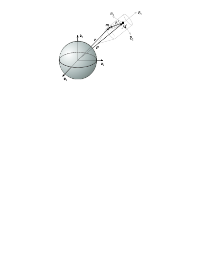
Figure 1: A harmonically trapped particle with position $\mathbf{r}$ and mass $m$ falls towards the Earth in a drop capsule with position $\bm{\rho}$ and mass $\mathcal{M}$. The center-of-mass of the drop capsule $\bm{\rho}$ and its major axes coincide also with the origin of the harmonic trap and its principal axes $\mathbf{\widetilde{e}}_{i}$.

II.1.2 Hamiltonian dynamics

In considering the mass $\mathcal{M}$ of the drop capsule, it is clear that classical mechanics rules its dynamics. The succinct formulation of analytical mechanics follows from Hamilton’s principle, which demands that the trajectory defined by position $\bm{\rho}$ and orientation of the capsule $\mathbf{n}$, extremizes the classical action

$$S_{c}[\bm{\rho},\mathbf{n}]=\int_{t_{0}}^{t}\text{d}t^{\prime}\,L_{c}[\bm{\rho}(t^{\prime}),\dot{\bm{\rho}}(t^{\prime}),\dot{\mathbf{n}}(t^{\prime}),t^{\prime}],$$ (2)

subject to appropriate boundary conditions Goldstein (1981). The Lagrangian for the drop capsule $L_{c}$ with respect to an inertial frame is given by

$$L_{c}[\bm{\rho},\dot{\bm{\rho}},\dot{\mathbf{{n}}},t]=\mathcal{M}\left(\frac{\dot{\bm{\rho}}^{2}}{2}-V_{g}(\bm{\rho},t)\right)+\frac{1}{2}\dot{\mathbf{n}}\,\mathcal{I}\,\dot{\mathbf{n}}.$$ (3)

In there, we introduced the tensor of inertia $\mathcal{I}$. The rate of change of $\mathbf{n}$ corresponds to the angular velocity or spinning of the capsule. As mentioned in the introduction, we will disregard possible torques, which arise due to weak gravity inhomogeneities. Thus, the internal angular momentum of the drop capsule is conserved $\mathcal{I}\dot{\mathbf{n}}=\text{const.}$, in other words $\mathbf{n}$ is a cyclic variable in the Lagrangian Eq. (3). To simplify the following discussion, we will also drop the energy offset $\dot{\mathbf{n}}\,\mathcal{I}\,\dot{\mathbf{n}}/2$, which has no dynamical consequences.

The global extremum of the action $S_{c}$ is attained when the trajectory satisfies locally the Euler-Lagrange equations

$$\frac{d}{dt}\frac{\partial L_{c}}{\partial\dot{\bm{\rho}}}=\frac{\partial L_{c}}{\partial\bm{\rho}}.$$ (4)

The transition from the Lagrangian to the Hamiltonian formulation is based on the introduction of the canonical momenta

$$\bm{\pi}(\dot{\bm{\rho}}) =\frac{\partial L_{c}}{\partial\dot{\bm{\rho}}}=\mathcal{M}\dot{\bm{\rho}}.$$ (5)

Provided the canonical momenta can be expressed uniquely via velocities, then the Legendre transformation of the Lagrangian is invertible, $\text{Det}(\partial^{2}L_{c}/\partial\dot{\rho}_{i}\partial\dot{\rho}_{j})\neq 0$. It defines a Hamiltonian function in phase space

$$H_{c}(\bm{\rho},\bm{\pi},t) =\bm{\pi}\dot{\bm{\rho}}(\bm{\pi})-L_{c},$$ (6)

and the Hamiltonian equations of motion represent the dynamics

$$\dot{\bm{\rho}} =\frac{\partial H_{c}}{\partial\bm{\pi}}, \qquad\dot{\bm{\pi}} =-\frac{\partial H_{c}}{\partial\bm{\rho}}.$$ (7)

In particular, applying analytical mechanics to the drop capsule in vacuum, falling in gravity, we find

$$\dot{\bm{\rho}} =\frac{\bm{\pi}}{\mathcal{M}}, \qquad\dot{\bm{\pi}} =-\mathcal{M}\frac{\partial}{\partial\bm{\rho}}V_{g}(\bm{\rho},t),$$ (8)

or simply Newton’s equation

$$\ddot{\bm{\rho}}=-\frac{\partial}{\partial\bm{\rho}}V_{g}(\bm{\rho},t).$$ (9)

II.2 A single classical particle trapped in the drop capsule

For our considerations the inertial frame of reference as well as the comoving frame of the drop capsule are of significance. Therefore, we will briefly discuss them in the following sections.

II.2.1 Inertial frame

The situation considered in Fig. 1 is almost analogous to Newton’s proverbial apple dropping in the falling elevator. However, in addition to the gravitational acceleration, our particle with coordinate $\mathbf{r}$ experiences a linear trapping force, possibly time-dependent. This force is derived from a harmonic oscillator potential

$$V_{t}({\bm{\xi}},t)= \frac{1}{2}\,({\bm{\xi}}\otimes{\bm{\xi}})\cdot v_{t}^{(2)}(t),$$ (10)

$$v_{t}^{(2)}(t)= \sum_{i=1}^{3}\omega_{i}^{2}(t)\ \mathbf{\widetilde{e}}_{i}\otimes\mathbf{\widetilde{e}}_{i},$$ (11)

which is tied to the center-of-mass of the drop capsule $\bm{\rho}$ and is rigidly aligned along the symmetry axes of the capsule $\{\mathbf{\widetilde{e}}_{1},\mathbf{\widetilde{e}}_{2},\mathbf{\widetilde{e}}_{3}\}$. In general, the potential can be anisotropic with time-dependent trap frequencies $\omega_{i}(t)$. Both information is incorporated in the definition of the symmetric tensor $v_{t}^{(2)}(t)$.

As before, the equation of motion for the falling, trapped particle follows straight from the Lagrangian of the drop capsule, Eq. (3), by adding the corresponding Lagrangian of the trapped particle

$$L[\bm{\rho},\dot{\bm{\rho}},\mathbf{r},\dot{\mathbf{r}},t]=L_{c}[\bm{\rho},\dot{\bm{\rho}},t]+L_{sp}[\mathbf{r},\dot{\mathbf{r}},t],$$ (12)

$$L_{sp}[\mathbf{r},\dot{\mathbf{r}},t]=m\left(\frac{\dot{\mathbf{r}}^{2}}{2}-V_{t}(\mathbf{r}-\bm{\rho}(t),t)-V_{g}(\mathbf{r},t)\right).$$ (13)

It almost goes without saying that the back-action of the particle on the drop capsule is negligible, since the mass of the drop capsule $\mathcal{M}\gg m$ is much larger than the mass $m$ of the atomic particle.

In the inertial frame, the atomic canonical momentum ${\mathbf{p}}$ is identical with the kinetic momentum

$${\mathbf{p}}=\frac{\partial L_{sp}}{\partial\dot{\mathbf{r}}}=m\dot{\mathbf{r}}.$$ (14)

Thus, the Hamiltonian function for the single trapped particle is obtained immediately as

$$H {}_{sp}(\mathbf{r},{\mathbf{p}},t)={\mathbf{p}}\dot{\mathbf{r}}-L_{sp}$$ (15)

$$=\frac{{\mathbf{p}}^{2}}{2m}+m[V_{{t}}\left(\mathbf{r}-\bm{\rho}(t),t\right)+V_{g}(\mathbf{r},t)]$$

and the equations of motion read as

$$\dot{\mathbf{r}}=\frac{{\mathbf{p}}}{m},$$ (16)

$$\dot{{\mathbf{p}}}=-m\frac{\partial}{\partial\mathbf{r}}[V_{{t}}\left(\mathbf{r}-\bm{\rho}(t),t\right)+V_{g}(\mathbf{r},t)].$$ (17)

This yields Newton’s equation for the particle coordinates $\mathbf{r}$

$$\ddot{\mathbf{r}}=-\frac{\partial}{\partial\mathbf{r}}\left[V_{t}\left(\mathbf{r}-\bm{\rho}(t),t\right)+V_{g}(\mathbf{r},t)\right].$$ (18)

II.2.2 Comoving frame

The particle can deviate only a tiny distance from the center of the drop capsule. It is of the order of $1$ cm, hence much less than the radius of the Earth. Consequently, it is prudent to make a coordinate transformation to the comoving, accelerated frame and also to introduce relative velocities

$$\mathbf{r}^{\prime} =\mathbf{r}-\bm{\rho}(t),\qquad\dot{\mathbf{r}}^{\prime}=\dot{\mathbf{r}}-\dot{\bm{\rho}}.$$ (19)

The Lagrangian of the particle now reads

$$L_{sp}^{\prime}[\mathbf{r}^{\prime},\dot{\mathbf{r}}^{\prime},t]=m\left(\frac{(\dot{\mathbf{r}}^{\prime}+\dot{\bm{\rho}})^{2}}{2}-V_{t}(\mathbf{r}^{\prime},t)-V_{g}(\mathbf{r}^{\prime}+\bm{\rho},t)\right)$$ (20)

and induces a canonical momentum as

$${\mathbf{p}}^{\prime}=\frac{\partial L_{sp}^{\prime}}{\partial\dot{\mathbf{r}}^{\prime}}=m(\dot{\mathbf{r}}^{\prime}+\dot{\bm{\rho}}).$$ (21)

Now, the Hamiltonian in the accelerated frame is given by

$$H_{sp}^{\prime}( \mathbf{r}^{\prime},{\mathbf{p}}^{\prime},t)={\mathbf{p}}^{\prime}\dot{\mathbf{r}}^{\prime}-L_{sp}^{\prime}$$ (22)

$$=\frac{{\mathbf{p}}^{\prime 2}}{2m}+m[V_{{t}}\left(\mathbf{r}^{\prime},t\right)+V_{g}(\mathbf{r}^{\prime}+\bm{\rho},t)]-{\mathbf{p}}^{\prime}\dot{\bm{\rho}}.$$

and leads to the following equations of motion

$$\dot{\mathbf{r}}^{\prime} =\frac{\partial H_{sp}^{\prime}}{\partial{\mathbf{p}}^{\prime}}=\frac{{\mathbf{p}}^{\prime}}{m}-\dot{\bm{\rho}},$$ (23)

$$\dot{{\mathbf{p}}}^{\prime} =-\frac{\partial H_{sp}^{\prime}}{\partial\mathbf{r}^{\prime}}=-m\frac{\partial}{\partial\mathbf{r}^{\prime}}[V_{{t}}\left(\mathbf{r}^{\prime},t\right)+V_{g}(\mathbf{r}^{\prime}+\bm{\rho},t)],$$ (24)

or Newton’s equation

$$\ddot{\mathbf{r}}^{\prime} =-\frac{\partial}{\partial\mathbf{r}^{\prime}}\left[V_{{t}}\left(\mathbf{r}^{\prime},t\right)+V_{g}(\mathbf{r}^{\prime}+\bm{\rho},t)\right]-\ddot{\bm{\rho}}.$$ (25)

Due to the smallness of the possible deviation of the trapped particle from the trap center, we can safely expand the gravitational potential at each instant in a Taylor series along the trajectory of the drop capsule $\bm{\rho}(t)$,

$$\begin{gathered}V_{g}(\mathbf{r^{\prime}}+\bm{\rho},t)=[1+\mathbf{r^{\prime}}\,\frac{\partial}{\partial\bm{\rho}}+\frac{1}{2!}(\mathbf{r^{\prime}}\,\frac{\partial}{\partial\bm{\rho}})^{2}+\ldots]\,V_{g}(\bm{\rho},t)\\ =V_{g}(\bm{\rho},t)+V_{g}^{(1)}(\mathbf{r}^{\prime},\bm{\rho},t)+V_{g}^{(2)}(\mathbf{r}^{\prime},\bm{\rho},t)\\ +\delta V_{g}^{(3)}(\mathbf{r}^{\prime},\bm{\rho},t).\end{gathered}$$ (26)

This expansion defines the gradient field and a linear potential contribution,

$$\begin{aligned} \mathbf{v}_{g}^{(1)}(\bm{\rho},t)&=\frac{\partial}{\partial\bm{\rho}}\,V_{g}(\bm{\rho},t),\\ V_{g}^{(1)}(\mathbf{r}^{\prime},\bm{\rho},t)&=\mathbf{r}^{\prime}\ \mathbf{v}_{g}^{(1)}(\bm{\rho},t),\end{aligned}$$ (27)

the symmetric Hessian tensor and its complete contraction into a quadratic potential energy

$$\begin{aligned} v_{g}^{(2)}(\bm{\rho},t)&=(\frac{\partial}{\partial\bm{\rho}}\otimes\frac{\partial}{\partial\bm{\rho}})\ V_{g}(\bm{\rho},t),\\ V_{g}^{(2)}(\mathbf{r}^{\prime},\bm{\rho},t)&=\frac{1}{2}\,(\mathbf{r}^{\prime}\otimes\mathbf{r}^{\prime})\cdot v_{g}^{(2)}(\bm{\rho},t),\end{aligned}$$ (28)

as well as a residual correction $\delta V_{g}^{(3)},$ given in Appendix A. Due to its smallness, we will tacitly disregard corrections of this order in all of the following considerations.

II.2.3 Pre-release dynamics

Prior to the release at $t_{0}$, the capsule is statically attached to the top of the tower, i.e. $\dot{\bm{\rho}}(t<t_{0})=0$, at some hight $\bm{\rho}_{0}$. Please note that the vanishing velocity implies that we have deliberately “frozen” the rotation of the Earth. This is rectified in Sec. IV. Then, we can approximate Newton’s equation Eq. (25) as

$$\ddot{\mathbf{r}}^{\prime} =-\frac{\partial}{\partial\mathbf{r}^{\prime}}\tilde{V}_{t}(\mathbf{r}^{\prime},\bm{\rho}_{0},t)-\mathbf{v}^{(1)}_{g}(\bm{\rho}_{0},t),$$

$$=-\,\tilde{v}^{(2)}_{t}(\bm{\rho}_{0},t)\,(\mathbf{r}^{\prime}-\mathbf{r}^{\prime}_{eq}(t)).$$ (29)

The equilibrium position $\mathbf{r}^{\prime}_{eq}$ reflects the gravitational sag of the particle with respect to the trap center $\bm{\rho}_{0}$ at some instant and is given by

$$\tilde{v}^{(2)}_{t}(\bm{\rho}_{0},t)\,\mathbf{r}^{\prime}_{eq}(t)=-\mathbf{v}^{(1)}_{g}(\bm{\rho}_{0},t).$$ (30)

Presumably, its time dependence is very slow. Furthermore, we have gathered all quadratic potential energy contributions into a renormalized harmonic trapping potential as

$$\begin{gathered}\tilde{v}^{(2)}_{t}(\bm{\rho},t)=v_{t}^{(2)}(t)+v_{g}^{(2)}(\bm{\rho},t),\\ \tilde{V}_{t}({\bm{\xi}},\bm{\rho},t)=\frac{1}{2}\,({\bm{\xi}}\otimes{\bm{\xi}})\cdot\tilde{v}^{(2)}_{t}(\bm{\rho},t).\end{gathered}$$ (31)

It is interesting to note that the trapping force is weakened in the direction of gravity as the curvature coefficients $v_{g}^{(2)}$ are negative.

II.2.4 Post-release dynamics

After the capsule is released, i. e., for times $t>t_{0}$, it falls essentially according to Eq. (9). Due to the previously mentioned sag in the direction of gravity, the equilibrated atomic particle will be in a position $\mathbf{r}^{\prime}(t_{0})=\mathbf{r}^{\prime}_{eq}(t_{0})$ and initiate harmonic oscillations about the instantaneous trap center $\bm{\rho}(t)$

$$\ddot{\mathbf{r}}^{\prime} =-\frac{\partial}{\partial\mathbf{r}^{\prime}}\ \tilde{V}_{t}(\mathbf{r}^{\prime},\bm{\rho}(t),t)=-\tilde{v}^{(2)}_{t}(\bm{\rho}(t),t)\,\mathbf{r}^{\prime}.$$ (32)

II.2.5 Hamiltonian formulation and canonical transformations

In order to obtain the transformed single-particle Hamilton function $H^{\prime}_{sp}(\mathbf{r}^{\prime},{\mathbf{p}}^{\prime},t)$ in terms of the old Hamilton function $H_{sp}(\mathbf{r},{\mathbf{p}},t)$ of Eq. (15), we used the coordinate transformation of Eq. (19) and stepped through the Lagrangian procedure. More elegantly, one can also employ the general approach of canonical transformations Goldstein (1981). In particular, we will choose a time-dependent generating function

$$G(\mathbf{r},{\mathbf{p}}^{\prime\prime},t)=[\mathbf{r}-\bm{\rho}(t)]{\mathbf{p}}^{\prime\prime}+\frac{m}{\mathcal{M}}[s(t)+\mathbf{r}\bm{\pi}(t)]$$ (33)

that depends explicitly on the old particle coordinate and the new momentum variable $\{\mathbf{r},{\mathbf{p}}^{\prime\prime}\}$. It also depends parametrically on the coordinate and momentum of the drop capsule $\{\bm{\rho}(t),\bm{\pi}(t)\}$. For convenience, another, yet undetermined variable $s(t)$ was introduced. This does not affect the dynamics at all, but can be used to match the energy-zero level at some instant. The new coordinate $\mathbf{r}^{\prime\prime}$ and the old momentum ${\mathbf{p}}$ are obtained from the generating function as

$$\mathbf{r}^{\prime\prime} =\frac{\partial G}{\partial{\mathbf{p}}^{\prime\prime}}=\mathbf{r}-\bm{\rho}(t), \quad{\mathbf{p}} =\frac{\partial G}{\partial\mathbf{r}}={\mathbf{p}}^{\prime\prime}+\frac{m}{\mathcal{M}}\bm{\pi}(t).$$ (34)

Note that besides the displacement of the coordinate $\mathbf{r}$, we also introduced a boost in momentum space, which differs from the transformation described by Eq. (19). With respect to the transformed frame, the new Hamiltonian reads formally as

$$H^{\prime\prime}_{sp}( \mathbf{r}^{\prime\prime},{\mathbf{p}}^{\prime\prime},t)=H_{sp}(\mathbf{r},{\mathbf{p}},t)+\frac{\partial}{\partial t}G(\mathbf{r},{\mathbf{p}}^{\prime\prime},t).$$ (35)

By inserting the coordinate transformation as well as employing the Taylor expansion of the gravitational potential, we find the residual harmonic Hamiltonian

$$H^{\prime\prime}_{sp}(\mathbf{r}^{\prime\prime},{\mathbf{p}}^{\prime\prime},t)=\frac{{{\mathbf{p}}^{\prime\prime}}^{2}}{2m}+m\tilde{V}_{t}(\mathbf{r}^{\prime\prime},\bm{\rho}(t),t),$$ (36)

provided the motion of the capsule is externally determined by the solution of Eq. (8) and $s(t,t_{0})$ is an action

$$s(t,t_{0})=\int_{t_{0}}^{t}\text{d}t^{\prime}L_{c}[\bm{\rho}(t^{\prime}),\dot{\bm{\rho}}(t^{\prime}),t^{\prime}]-\bm{\rho}\pi|^{t}_{t_{0}}.$$ (37)

By construction it is clear that we must recover the identical Eq. (32) from Hamilton’s equations in the new coordinates

$$\dot{\mathbf{r}}^{\prime\prime} =\frac{\partial H^{\prime\prime}_{sp}}{\partial{\mathbf{p}}^{\prime\prime}}, \qquad\dot{{\mathbf{p}}}^{\prime\prime} =-\frac{\partial H^{\prime\prime}_{sp}}{\partial\mathbf{r}^{\prime\prime}}.$$ (38)

We would like to point out that these considerations are not purely academic but will enlighten the analogy between the classical treatment and the quantum mechanical description of the falling, trapped ultra-cold quantum gas.

II.2.6 Order of magnitude estimates

In order to estimate the magnitude of the Taylor coefficients of the gravitational potential, one can evaluate them at the surface of the Earth $\rho=R_{\small\earth}=6372$ km and obtains $v_{g}^{(1)}=9.81\ \mbox{m}\,\mbox{s}^{-2}$, $v_{g}^{(2)}=-1.54\times 10^{-6}\ \mbox{s}^{-2}$ and $v_{g}^{(3)}=2.42\times 10^{-13}\ \mbox{m}^{-1}\,\mbox{s}^{-2}$. In there, we made the approximation of an isotropic gravitational potential. It is worthwhile pointing out that $v_{g}^{(1)}$ is not yet identical to the gravitational acceleration $g$, which also includes centrifugal corrections (see Sec. IV).

The important consequence of Eq. (32) is that in first order $V_{g}^{(1)}$, the internal harmonic oscillator motion is decoupled from the center-of-mass motion of the drop capsule. Only when considering the weak quadratic correction $V_{g}^{(2)}$, one can observe a coupling of these motions as a result of the decrease of the harmonic oscillator frequency along the gradient of the gravitation. The following quantum mechanical calculations will obviously lead to the same conclusions due to Ehrenfest’s theorem, where in case of quadratic Hamiltonians expectation values coincide with the classical trajectories. Only by considering the third order correction $\delta V_{g}^{(3)}$, we will find an additional dynamical mixing between the classical trajectory and the quantum mechanical expectation value.

III Quantum physics of identical atoms falling within the drop capsule

So far, we have considered a single classical particle that is harmonically trapped and falling in the gravitational field. Actually, we are interested in the behavior of a freely falling, trapped atomic Bose-Einstein condensate (BEC), which requires a quantum field theoretical description. However, we do not want to constrain our discussion solely to condensed bosonic gases, but would rather like to treat the general situation of an ultra-cold degenerate quantum gas, whether bosonic or fermionic.

III.1 Quantized atomic fields

Before we proceed to the quantum field theoretical description, which is intrinsically tied to the picture of second quantization, we briefly revisit the most prominent relations of first quantization. In general, the commutator of position and momentum operator $\hat{\mathbf{r}}$ and $\hat{\mathbf{p}}$ is

$$[\hat{\mathbf{r}},\hat{\mathbf{p}}]=i\hbar\,\mathds{1}.$$ (39)

In the remainder of this article, we will omit the hats for operators in first quantization, e.g. write $\mathbf{r}$ and ${\mathbf{p}}$. The derived commutation relation for the components of the angular momentum $\mathbf{l}=\mathbf{r}\times{\mathbf{p}}$ satisfies the standard angular momentum algebra

$$[l_{k},l_{l}]=i\hbar\,\epsilon_{klm}\,l_{m},$$ (40)

defined through the completely anti-symmetric Levi-Civita tensor $\epsilon_{klm}$ as structure constants. Most of the time, we will use the position representation in this article, hence will interchangeably refer to $\mathbf{r}$ and ${\mathbf{p}}=-i\hbar\frac{\partial}{\partial\mathbf{r}}$ also as the operators of position and momentum, when acting on Hilbert-space functions.

In order to incorporate the correct quantum statistics according to the Pauli principle, we use the language of second quantization and introduce the basic quantities in the following. The field operator in the position representation will be denoted by ${\hat{a}^{\vphantom{{\dagger}}}(\mathbf{r})}$ and it annihilates a particle at the position $\mathbf{r}$, while its hermitian conjugate ${\hat{a}^{{\dagger}}(\mathbf{r})}$ creates it there. In the present discussion, all operators are given in the Schrödinger picture unless indicated otherwise. Thus, the quantum field satisfies a commutation relation for bosons $(-)$ and an anti-commutation rule for fermions $(+)$

$$\left[\hat{a}(\mathbf{r}),\hat{a}^{\dagger}(\mathbf{r}^{\prime})\right]_{\mp}=\delta\left(\mathbf{r}-\mathbf{r}^{\prime}\right).$$ (41)

For commutators, we will drop the “$-$” in the following.

Now, we can proceed to single-particle operators in Fock space representing the center-of-mass coordinate ${\hat{\mathbf{R}}}$, the linear momentum ${\hat{\mathbf{P}}}$, as well as the angular momentum ${\hat{\mathbf{L}}}$ and the total atom number ${\hat{N}}$ as

$$\begin{gathered}{\hat{\mathbf{R}}}=\int\,\text{d}^{3}r\,{\hat{a}^{{\dagger}}(\mathbf{r})}\,\mathbf{r}\,{\hat{a}^{\vphantom{{\dagger}}}(\mathbf{r})},\ \ {\hat{\mathbf{P}}}=\int\,\text{d}^{3}r\,{\hat{a}^{{\dagger}}(\mathbf{r})}\,{\mathbf{p}}\,{\hat{a}^{\vphantom{{\dagger}}}(\mathbf{r})},\\ {\hat{\mathbf{L}}}=\int\,\text{d}^{3}r\,{\hat{a}^{{\dagger}}(\mathbf{r})}\,\mathbf{l}\,{\hat{a}^{\vphantom{{\dagger}}}(\mathbf{r})},\ \ \hat{N}=\int\,\text{d}^{3}r\,{\hat{a}^{{\dagger}}(\mathbf{r})}\,{\hat{a}^{\vphantom{{\dagger}}}(\mathbf{r})}.\\ \end{gathered}$$ (42)

Using the commutation or anti-commutation relation of Eq. (41), one can easily verify that those operators form a closed algebra

$$\left[{\hat{\mathbf{R}}},{\hat{\mathbf{P}}}\right]=i\hbar\,{\hat{N}},$$ (43)

$$\left[{\hat{\mathbf{R}}},{\hat{N}}\right]=\left[{\hat{\mathbf{P}}},{\hat{N}}\right]=\left[{\hat{\mathbf{L}}},{\hat{N}}\right]=0,$$ (44)

$$\left[{\hat{\mathbf{R}}},\bm{\Omega}{\hat{\mathbf{L}}}\right]=i\hbar\ \bm{\Omega}\times{\hat{\mathbf{R}}},\quad\left[{\hat{\mathbf{P}}},\bm{\Omega}{\hat{\mathbf{L}}}\right]=i\hbar\ \bm{\Omega}\times{\hat{\mathbf{P}}}.$$ (45)

It is indicated by Eq. (44) that this algebra of Euclidean transformations can be represented in the $N$-particle sector and $\bm{\Omega}$ represents an arbitrary rotational axis in three-dimensional Euclidean space.

In typical BEC experiments, as well as in recent experiments involving degenerate fermions, the particle densities are of the order $10^{13}$ cm^-3. Thus, we can express the energy of a dilute atomic gas of $N$ particles in form of a cluster expansion

$$\begin{gathered}H^{(N)}(t)=\sum_{i=1}^{N}H_{{sp}}(\mathbf{r}_{i},{\mathbf{p}}_{i},t)+\sum_{i<j}^{N}V_{p}(\mathbf{r}_{i}-\mathbf{r}_{j})\end{gathered}$$ (46)

in terms of single-particle Hamiltonians $H_{sp}(\mathbf{r},{\mathbf{p}},t)$, pair-wise interactions $V_{p}({\bm{\xi}})$ and, with decreasing relevance, higher order effects, which can be neglected here Pethick and Smith (2002); Pitaevskii and Stringari (2003). The recently discovered Efimov-resonances Kraemer et al. (2006) represent a very unusual exception to this rule, where genuine three-body effects become important. However, the principle of translational invariance can still be assumed for those potentials. For the present discussion, we will disregard such peculiarities, however. Obviously, we want to assume in here that the quantum dynamics of the $N$-particle state follows the $N$-particle Schrödinger equation

$$\begin{gathered}i\hbar\,\frac{d}{dt}|\Psi^{(N)}\rangle=H^{(N)}(t)\,|\Psi^{(N)}\rangle.\end{gathered}$$ (47)

Now, if this is translated to the view point of second quantization, one obtains the standard Hamilton operator

$$\begin{gathered}\hat{H}(t)=\hat{H}_{sp}(t)+\hat{V}_{p},\\ \hat{H}_{sp}(t)=\int\,\text{d}^{3}r\,{\hat{a}^{{\dagger}}(\mathbf{r})}H_{{sp}}(\mathbf{r},{\mathbf{p}},t){\hat{a}^{\vphantom{{\dagger}}}(\mathbf{r})},\\ \hat{V}_{p}=\frac{1}{2}\int\text{d}^{6}r\ {\hat{a}^{{\dagger}}(\mathbf{r}_{1})}{\hat{a}^{{\dagger}}(\mathbf{r}_{2})}V_{p}(\mathbf{r}_{1}-\mathbf{r}_{2}){\hat{a}^{\vphantom{{\dagger}}}(\mathbf{r}_{2})}{\hat{a}^{\vphantom{{\dagger}}}(\mathbf{r}_{1})}.\end{gathered}$$ (48)

In low-energy field theory, the pair potential $V_{p}$ is often modeled not by a finite range potential, but it is assumed to be proportional to a delta function. This is called the contact- or pseudo-potential approximation. It is very useful in certain situations, but needs careful consideration when going to higher order calculations Abrikosov et al. (1965). For the present discussion, we can postpone this question and simply demand translational invariance.

In principle, one can represent any state in Fock space as

$$\begin{gathered}\left|\Psi\right\rangle=\sum_{N=0}^{\infty}\int\text{d}^{3N}r\,\left|\mathbf{r}_{1},\ldots,\mathbf{r}_{N}\right\rangle\langle\mathbf{r}_{1},\ldots,\mathbf{r}_{N}\!\mid\!\Psi^{(N)}\rangle,\\ \left|\mathbf{r}_{1},\ldots,\mathbf{r}_{N}\right\rangle={\hat{a}^{{\dagger}}(\mathbf{r}_{1})}\ldots{\hat{a}^{{\dagger}}(\mathbf{r}_{N})}\left|v\right\rangle,\end{gathered}$$ (49)

as a superposition of different $N$-particle states $\left|\mathbf{r}_{1},\ldots,\mathbf{r}_{N}\right\rangle$ created out of the vacuum $\left|v\right\rangle$ and weighted by the properly symmetrized or anti-symmetrized $N$-particle amplitudes $\Psi^{(N)}(\mathbf{r}_{1},\ldots,\mathbf{r}_{N})=\langle\mathbf{r}_{1},\ldots,\mathbf{r}_{N}\!\mid\!\Psi^{(N)}\rangle$.

Proceeding formally, it is also well-known that the complex-valued Lagrangian for Schrödinger fields Hill (1951); Gitman and Tyutin (1990); Kobe (2006)

$$\mathcal{L}[\Psi(t),\dot{\Psi}(t),t]=\left\langle\Psi(t)\right|i\hbar\frac{\partial}{\partial t}-\hat{H}(t)\left|\Psi(t)\right\rangle$$ (50)

leads via a Euler-Lagrange variational procedure

$$\Pi(t) =\frac{\delta\mathcal{L}}{\delta\dot{\Psi}}=i\hbar\,{\Psi}(t)^{\ast}, \quad\dot{\Pi}(t) =\frac{\delta\mathcal{L}}{\delta\Psi},$$ (51)

also to the Schrödinger equation in Fock space

$$i\hbar\,\frac{d}{dt}\left|\Psi(t)\right\rangle=\hat{H}(t)\,\left|\Psi(t)\right\rangle,$$ (52)

finally. With this fundamental equation of motion, we have now established all the basic concepts and can turn to the transformation of a wave function from an inertial frame of reference to an accelerated, comoving frame of reference.

III.2 Static representation of states in Euclidean frames of reference

In this subsection, we will briefly review basic transformation theory for wave functions under spatial translations and rotations of the coordinate system Gottfried (1966); Schmid (1977a, b); Klink (1997a, b).

III.2.1 Three-dimensional Euclidean space

The basic operation of a translation in space is given by

$$T_{\mathcal{R}}[\mathbf{r}]=\mathbf{r}+{\bm{\mathcal{R}}}.$$ (53)

The whole set of translational operators forms an Abelian group i. e., $T_{\mathcal{R}_{1}}T_{\mathcal{R}_{2}}=T_{\mathcal{R}_{1}+\mathcal{R}_{2}}$. Each element of this continuous Lie group is indexed by a three-dimensional vector ${\bm{\mathcal{R}}}$.

A rotation around an axis $\bm{\Omega}$ for a time $t$ is characterized by a total rotational vector ${\bm{\mathcal{Q}}}=\bm{\Omega}\,t$. This operation will be denoted by $M_{{\mathcal{Q}}}$. The set of all those isometric, linear transformations forms the infinite-dimensional Lie group ${\rm SO}(3)$, which excludes the possibility of reflections. The entirety of operations establishes the Euclidean group and a particular element is denoted by

$$\mathbf{r}^{\prime} = T_{\mathcal{R}}[M_{\mathcal{Q}}\,\mathbf{r}]=M_{\mathcal{Q}}\,\mathbf{r}+{\bm{\mathcal{R}}}.$$ (54)

If we represent the basic position vector in Cartesian coordinates as $\mathbf{r}=\sum_{i=1}^{3}r^{i}\mathbf{e}_{i}$, then one finds a three-dimensional orthogonal rotational matrix

$$M_{\mathcal{Q}}\,\mathbf{r} = e^{-i/\hbar\,{\bm{\mathcal{Q}}}\bm{\ell}}\ \mathbf{r}=\mathbf{r}+{\bm{\mathcal{Q}}}\times\mathbf{r}+\ldots,$$ (55)

in terms of the generators of the rotation $\{\ell_{1},\ell_{2},\ell_{3}\}$. For convenience, we have introduced those $3\times 3$-matrices as complex-valued angular momenta in units of $\hbar$, which satisfy the angular momentum algebra of Eq. (40). No quantum aspects are implied by this choice of notation (see also Appendix B).

III.2.2 Single-particle Hilbert space

The action of the translational operator in single-particle Hilbert space

$$U_{\mathcal{R}}=e^{-i/\hbar\,{\bm{\mathcal{R}}}{\mathbf{p}}},$$ (56)

can be seen most clearly by applying it to position eigenstates

$$\left|\mathbf{r}\right\rangle^{\prime}=U_{\mathcal{R}}\,\left|\mathbf{r}\right\rangle=\left|T_{\mathcal{R}}[\mathbf{r}]\right\rangle=\left|\mathbf{r}+{\bm{\mathcal{R}}}\right\rangle.$$ (57)

Obviously, the operation

$$U_{\mathcal{P}}=e^{i/\hbar\,{\bm{\mathcal{P}}}\mathbf{r}},$$ (58)

is just a boost in momentum space, when acting on momentum eigenstates, i. e.,

$$\left|{\mathbf{p}}\right\rangle^{\prime}=U_{\mathcal{P}}\,\left|{\mathbf{p}}\right\rangle=\left|T_{\mathcal{P}}[{\mathbf{p}}]\right\rangle=\left|{\mathbf{p}}+{\bm{\mathcal{P}}}\right\rangle.$$ (59)

The unitary representation of the rotation

$$U_{\mathcal{Q}}=e^{-i/\hbar\,{\bm{\mathcal{Q}}}\mathbf{l}},$$ (60)

is induced by the angular momentum operator $\mathbf{l}$ of Eq. (40). When acting on position as well as momentum eigenstates, one gets

$$\left|\mathbf{r}\right\rangle^{\prime}=U_{\mathcal{Q}}\,\left|\mathbf{r}\right\rangle=\left|M_{\mathcal{Q}}\,\mathbf{r}\right\rangle,$$ (61)

$$\left|{\mathbf{p}}\right\rangle^{\prime}=U_{\mathcal{Q}}\,\left|{\mathbf{p}}\right\rangle=\left|M_{\mathcal{Q}}\,{\mathbf{p}}\right\rangle.$$ (62)

Thus, a representation of a general element of the Euclidean group in Hilbert space is

$$U=U_{\mathcal{S}}\,U_{\mathcal{P}}\,U_{\mathcal{R}}\,U_{\mathcal{Q}},\quad U_{\mathcal{S}}=e^{i/\hbar\,{\mathcal{S}}}.$$ (63)

This definition of a general group element is not unique, but admits the inclusion of an arbitrary phase factor $U_{\mathcal{S}}$, such that the transformed position state reads

$$\left|\mathbf{r}\right\rangle^{\prime}=U\,\left|\mathbf{r}\right\rangle=e^{i/\hbar\,[{\mathcal{S}}+{\bm{\mathcal{P}}}(M_{\mathcal{Q}}\mathbf{r}+{\bm{\mathcal{R}}})]}\,\left|M_{\mathcal{Q}}\mathbf{r}+{\bm{\mathcal{R}}}\right\rangle.$$ (64)

Such a ray-representation will become physically important when considering the dynamic evolution of a quantum state, and the accumulated phase will reflect the classical action.

III.2.3 Many-particle Fock space

We will now proceed to a wave-function $\left|\Psi\right\rangle$ in many-particle Fock space and transform it to the wave-function $\left|\Psi\right\rangle^{\prime}$ in another Euclidean coordinate system

$$\left|\Psi\right\rangle={\hat{U}^{\vphantom{\dagger}}}\left|\Psi\right\rangle^{\prime}.$$ (65)

A general element of the Euclidean group in Fock space

$${\hat{U}^{\vphantom{\dagger}}}={\hat{U}_{\mathcal{S}}^{\vphantom{\dagger}}}{\hat{U}_{\mathcal{P}}^{\vphantom{\dagger}}}{\hat{U}_{\mathcal{R}}^{\vphantom{\dagger}}}{\hat{U}_{{\mathcal{Q}}}^{\vphantom{\dagger}}},$$ (66)

is now given by the following representation

$$\begin{aligned} {\hat{U}_{\mathcal{R}}^{\vphantom{\dagger}}}&=e^{-i/\hbar\,{\bm{\mathcal{R}}}\,{\hat{\mathbf{P}}}},&\qquad{\hat{U}_{\mathcal{P}}^{\vphantom{\dagger}}}&=e^{i/\hbar\,{\bm{\mathcal{P}}}\,{\hat{\mathbf{R}}}},\\ {\hat{U}_{\mathcal{S}}^{\vphantom{\dagger}}}&=e^{i/\hbar\,{\mathcal{S}}\,{\hat{N}}},&\qquad{\hat{U}_{{\mathcal{Q}}}^{\vphantom{\dagger}}}&=e^{-i/\hbar\,{\bm{\mathcal{Q}}}\,{\hat{\mathbf{L}}}},\end{aligned}$$ (67)

where the single-particle operators ${\hat{\mathbf{R}}},{\hat{\mathbf{P}}},{\hat{\mathbf{L}}}$ and ${\hat{N}}$ have been introduced in Eq. (42).

In the following context, we will not need the action of operators $\hat{U}$ on state vectors $\left|\Psi\right\rangle$ in Fock space, but rather on the scalar amplitudes of the quantum field in the position representation ${\hat{a}^{\vphantom{{\dagger}}}(\mathbf{r})}$. This is straight forward using the commutator relations of Appendix B in case of the phase operator ${\hat{U}_{\mathcal{S}}^{\vphantom{\dagger}}}$ and momentum boost operator ${\hat{U}_{\mathcal{P}}^{\vphantom{\dagger}}}$

$${\hat{U}_{\mathcal{S}}^{\dagger}}\,{\hat{a}^{\vphantom{{\dagger}}}(\mathbf{r})}\,{\hat{U}_{\mathcal{S}}^{\vphantom{\dagger}}}=U_{\mathcal{S}}\,{\hat{a}^{\vphantom{{\dagger}}}(\mathbf{r})},\quad{\hat{U}_{\mathcal{P}}^{\dagger}}\,{\hat{a}^{\vphantom{{\dagger}}}(\mathbf{r})}\,{\hat{U}_{\mathcal{P}}^{\vphantom{\dagger}}}=U_{\mathcal{P}}\,{\hat{a}^{\vphantom{{\dagger}}}(\mathbf{r})}.$$ (68)

For the spatial shift operator ${\hat{U}_{\mathcal{R}}^{\vphantom{\dagger}}}$ as well as the rotational operator ${\hat{U}_{{\mathcal{Q}}}^{\vphantom{\dagger}}}$, we need to recall that we are dealing with a scalar field. Then one finds that the unitary operations in single-particle Hilbert space $U_{\mathcal{R}}$ and $U_{\mathcal{Q}}$ correspond to the inverse operations in Euclidean space $T_{\mathcal{R}}^{-1}$ and $M_{\mathcal{Q}}^{-1}$, i. e.,

$${\hat{U}_{\mathcal{R}}^{\dagger}}\,{\hat{a}^{\vphantom{{\dagger}}}(\mathbf{r})}\,{\hat{U}_{\mathcal{R}}^{\vphantom{\dagger}}}=U_{\mathcal{R}}\,{\hat{a}^{\vphantom{{\dagger}}}(\mathbf{r})}={\hat{a}^{\vphantom{{\dagger}}}(T_{\mathcal{R}}^{-1}\mathbf{r})}={\hat{a}^{\vphantom{{\dagger}}}(\mathbf{r}-{\bm{\mathcal{R}}})},$$ (69)

$${\hat{U}_{\mathcal{Q}}^{\dagger}}\,{\hat{a}^{\vphantom{{\dagger}}}(\mathbf{r})}\,{\hat{U}_{{\mathcal{Q}}}^{\vphantom{\dagger}}}=U_{{\mathcal{Q}}}^{\vphantom{{\dagger}}}\,{\hat{a}^{\vphantom{{\dagger}}}(\mathbf{r})}={\hat{a}^{\vphantom{{\dagger}}}(M_{\mathcal{Q}}^{-1}\,\mathbf{r})}.$$ (70)

III.3 Dynamics in comoving frames of reference

III.3.1 Frame transformation from the inertial to the comoving frame

The Euclidean coordinate transformations of the previous section where determined by ten static parameters, $\{{\mathcal{S}},{\bm{\mathcal{R}}},{\bm{\mathcal{P}}},{\bm{\mathcal{Q}}}\}$. By considering an arbitrary time-dependence of these parameters, we can introduce a canonical frame transformation that includes the Galilean transformation as a special case Gottfried (1966). Currently, we will focus on non-rotating frames (${\bm{\mathcal{Q}}}=0$) for simplicity, i. e.,

$${\hat{U}^{\vphantom{\dagger}}}(t)=\hat{U}_{\mathcal{S}(t)}\,\hat{U}_{\mathcal{P}(t)}\,\hat{U}_{\mathcal{R}(t)}$$ (71)

and lift this restriction in Sec. IV.

Our goal is to determine an equation of motion for this comoving, accelerated frame such that the residual motion of the atomic gas within the frame is free of any non-inertial forces. Given the Schrödinger equation (52) holds in the inertial Earth-centered frame, then we find another realization $\left|\Psi\right\rangle={\hat{U}^{\vphantom{\dagger}}}(t)\left|\Psi(t)\right\rangle^{\prime}$ in an accelerated frame of reference

$$i\hbar\,\frac{d}{dt}\left|\Psi(t)\right\rangle^{\prime}=\hat{H}^{\prime}(t)\left|\Psi(t)\right\rangle^{\prime},$$ (72)

with the transformed Hamiltonian

$$\hat{H}^{\prime}(t)={\hat{U}^{\dagger}}(t)\,(-i\hbar\frac{d}{dt}+\hat{H}_{sp}(t)+\hat{V}_{p})\,{\hat{U}^{\vphantom{\dagger}}}(t).$$ (73)

In here, the first contribution to the Hamiltonian is a gauge potential, in analogy to the fictitious forces that would appear in the classical Hamiltonian function in terms of the time derivative of the generating function, cf. Eq. (35). It can be evaluated using Eqs. (193, 194) and it generates additional gauge forces

$${\hat{U}^{\dagger}}(t)(-i\hbar\frac{d}{dt}){\hat{U}^{\vphantom{\dagger}}}(t)=(\dot{{\mathcal{S}}}+\dot{{\bm{\mathcal{P}}}}{\bm{\mathcal{R}}})\,{\hat{N}}+\dot{{\bm{\mathcal{P}}}}\,{\hat{\mathbf{R}}}-\dot{{\bm{\mathcal{R}}}}\,{\hat{\mathbf{P}}}.$$ (74)

The second contribution to the Hamiltonian implements the spatial translation and momentum boost

$${\hat{U}^{\dagger}}(t)\,\hat{H}_{sp}(t)\,{\hat{U}^{\vphantom{\dagger}}}(t)$$ (75)

$$=\int\,\text{d}^{3}r^{\prime}\,{\hat{a}^{{\dagger}}(\mathbf{r}^{\prime})}\,H_{{sp}}(\mathbf{r}^{\prime}+{\bm{\mathcal{R}}},{\mathbf{p}}^{\prime}+{\bm{\mathcal{P}}},t)\,{\hat{a}^{\vphantom{{\dagger}}}(\mathbf{r}^{\prime})},$$

where it is implicitly assumed that the one-particle Hamiltonian $H_{sp}(\mathbf{r},{\mathbf{p}},t)$ can be expanded into a power series in $\mathbf{r}$ and $\mathbf{p}$, respectively.

The third term of the Hamiltonian Eq. (73) is not affected by the frame transformation,

$${\hat{U}^{\dagger}}\,\hat{V}_{p}\,{\hat{U}^{\vphantom{\dagger}}}=\hat{V}_{p},$$ (76)

as the interaction of Eq. (48) is hermitian (number conserving), a local operator, and translational invariant by construction in Fock-, as well as in two-particle Hilbert space,

$$[{\hat{N}},\hat{V}_{p}]=[{\hat{\mathbf{R}}},\hat{V}_{p}]=[{\hat{\mathbf{P}}},\hat{V}_{p}]=0.$$ (77)

This property is also the basis of Kohn’s theorem Kohn (1961), i. e., the exact decoupling of the center-of-mass motion and the relative excitations in maximally quadratic single-particle Hamiltonians. It is also known as the harmonic potential theorem Dobson (1994) and has been used in the context of cold dilute quantum gases Bialynicki-Birula and Z.Bialynicka-Birula (2002); Song (2005).

Combining these results, we find the transformed Hamiltonian in the accelerated frame

$$\hat{H}^{\prime}(t)=\int\,\text{d}^{3}r^{\prime}\,{\hat{a}^{{\dagger}}(\mathbf{r}^{\prime})}\,H_{sp}^{\prime}(\mathbf{r}^{\prime},{\mathbf{p}}^{\prime},t)\,{\hat{a}^{\vphantom{{\dagger}}}(\mathbf{r}^{\prime})}+\hat{V}_{p}$$ (78)

and all gauge contributions are contained in the single-particle Hamiltonian

$$\begin{split}H_{sp}^{\prime}(\mathbf{r}^{\prime},{\mathbf{p}}^{\prime},t)=&H_{sp}(\mathbf{r}^{\prime}+{\bm{\mathcal{R}}},{\mathbf{p}}^{\prime}+{\bm{\mathcal{P}}},t)\\ &+\dot{{\mathcal{S}}}+\dot{{\bm{\mathcal{P}}}}\,{\bm{\mathcal{R}}}+\dot{{\bm{\mathcal{P}}}}\,\mathbf{r}^{\prime}-\dot{{\bm{\mathcal{R}}}}\,{\mathbf{p}}^{\prime}.\end{split}$$ (79)

III.3.2 Application of the frame transformation in the harmonic approximation

We will now apply the preceeding considerations to the falling trapped interacting many-particle system in the drop tower. The single-particle Hamilton operator follows from the classical considerations of Eq. (15) and is given by

$$H_{sp}(\mathbf{r},{\mathbf{p}},t)=\frac{{\mathbf{p}}^{2}}{2\,m}+m\,[V_{{t}}\left(\mathbf{r}-\bm{\rho}(t),t\right)+V_{g}(\mathbf{r},t)].$$ (80)

By splitting the transformed Hamiltonian Eq. (79) into constant, linear and higher order polynomial contributions in terms of the position $\mathbf{r}^{\prime}$ and the momentum ${\mathbf{p}}^{\prime}$, one finds

$$\begin{gathered}H_{sp}^{\prime}(\mathbf{r}^{\prime},{\mathbf{p}}^{\prime},t)=(\bm{\alpha}{\mathbf{p}}^{\prime}+\bm{\beta}\mathbf{r}^{\prime}+\gamma)+\frac{{\mathbf{p}}^{\prime 2}}{2m}+mV_{{t}}\left(\mathbf{r}^{\prime},t\right)\\ +m\left[V_{g}(\mathbf{r}^{\prime}+{\bm{\mathcal{R}}},t)-V_{g}({\bm{\mathcal{R}}},t)-V_{g}^{(1)}(\mathbf{r}^{\prime},{\bm{\mathcal{R}}},t)\right]\end{gathered}$$ (81)

with coefficients

$$\bm{\alpha}= \frac{{\bm{\mathcal{P}}}}{m}-\dot{{\bm{\mathcal{R}}}},\quad\bm{\beta}=\dot{{\bm{\mathcal{P}}}}+m\,\frac{\partial}{\partial{\bm{\mathcal{R}}}}[V_{t}({\bm{\mathcal{R}}}-\bm{\rho},t)+V_{g}({\bm{\mathcal{R}}},t)],$$ (82)

$$\gamma= \frac{{\bm{\mathcal{P}}}^{2}}{2\,m}+m\,\left[V_{t}({\bm{\mathcal{R}}}-\bm{\rho},t)+V_{g}({\bm{\mathcal{R}}},t)\right]+\dot{{\mathcal{S}}}+\dot{{\bm{\mathcal{P}}}}\,{\bm{\mathcal{R}}}.$$

If the constraints are satisfied identically, i. e., $\{\bm{\alpha},\bm{\beta},\gamma\}\rightarrow 0$, one obtains the single-particle Hamiltonian, if we disregard again terms of third and higher orders $\delta V_{g}^{(3)}$ in the accelerated frame,

$$\begin{aligned} H_{sp}^{\prime}(\mathbf{r}^{\prime},{\mathbf{p}}^{\prime},t)=&\frac{{\mathbf{p}}^{\prime 2}}{2\,m}+m\,\widetilde{V}_{{t}}\left(\mathbf{r}^{\prime},{\bm{\mathcal{R}}}(t),t\right),\end{aligned}$$ (83)

provided the frame parameters as well as the center-of-mass of the drop capsule $\{{\bm{\mathcal{R}}}(t),{\bm{\mathcal{P}}}(t),\bm{\rho}(t)\}$ satisfy the classical equations of motion

$$\pi =\frac{\partial L_{c}}{\partial\dot{\bm{\rho}}}=\mathcal{M}\dot{\bm{\rho}}, \quad\dot{\pi} =\frac{\partial L_{c}}{\partial\bm{\rho}},$$ (84)

$${\bm{\mathcal{P}}} =\frac{\partial L_{sp}}{\partial\dot{{\bm{\mathcal{R}}}}}=m\dot{{\bm{\mathcal{R}}}}, \quad\dot{{\bm{\mathcal{P}}}} =\frac{\partial L_{sp}}{\partial{\bm{\mathcal{R}}}}.$$ (85)

We can express the latter line as Newton’s equation of motion for ${\bm{\mathcal{R}}}$,

$$\ddot{{\bm{\mathcal{R}}}}=-\frac{\partial}{\partial{\bm{\mathcal{R}}}}[V_{t}({\bm{\mathcal{R}}}-\bm{\rho},t)+V_{g}({\bm{\mathcal{R}}},t)].$$ (86)

With Eqs. (84) and (85), we have recovered the Lagrangian $L[\bm{\rho},\dot{\bm{\rho}},{\bm{\mathcal{R}}},\dot{{\bm{\mathcal{R}}}},t]$ of Eq. (12), and one can express the accrued dynamical phase as an action integral

$${\mathcal{S}}(t,t_{0})=\int_{t_{0}}^{t}dt^{\prime}L_{sp}[{\bm{\mathcal{R}}},\dot{{\bm{\mathcal{R}}}},t^{\prime}]-{\bm{\mathcal{P}}}{\bm{\mathcal{R}}}|^{t}_{t_{0}},$$ (87)

like in Eq. (2), where we started from, cf. also Eq. (37).

The harmonic trapping potential $\widetilde{V}_{{t}}$ that appears only in the residual Hamiltonian, Eq. (83), has been modified by quadratic corrections of gravity and was defined in Eq. (31). The third order correction to the gravitational potential $\delta V_{g}^{(3)}$ is minuscule. On the time scale of the free fall experiment, one may safely disregard it. Thus, we are left with a quadratic, time-dependent Hamilton operator and the harmonic potential theorem applies Dobson (1994).

As before, the motion of the center-of-mass coordinate ${\bm{\mathcal{R}}}$, Eq. (86), can be understood much more clearly, if we expand the gravitational potential around the center-of-mass of the drop capsule $\bm{\rho}$. For the deviation $\delta{\bm{\mathcal{R}}}(t)={\bm{\mathcal{R}}}(t)-\bm{\rho}(t)$ after the release of the capsule, one finds a pure harmonic oscillation

$$\delta\ddot{{\bm{\mathcal{R}}}}(t) =-\tilde{v}^{(2)}(\bm{\rho}(t),t)\,\delta{\bm{\mathcal{R}}}(t).$$ (88)

III.4 Ehrenfest’s theorem

At this point, we would like to confirm the physical interpretation of the frame parameters ${\bm{\mathcal{R}}}(t)$ and ${\bm{\mathcal{P}}}(t)$ as center-of-mass and momentum coordinates, respectively. Clearly, they have been introduced as such with dimensions of length and momentum. Using Ehrenfest’s theorem, we are able to verify this.

The temporal evolution of the expectation value of any time-independent operator $\hat{A}$, i. e., $\langle\hat{A}\rangle=\left\langle\Psi(t)\right|\hat{A}\left|\Psi(t)\right\rangle$ follows from the Schrödinger Eq. (52) and gives

$$i\hbar\,\frac{d}{dt}\langle\hat{A}\rangle=\langle[\hat{A},\hat{H}(t)]\rangle.$$ (89)

By using the bosonic or fermionic commutation relation, Eq. (41), we can work out the commutators in the Schrödinger picture

$$\frac{i}{\hbar}[\hat{H}(t),{\hat{\mathbf{R}}}]= \frac{{\hat{\mathbf{P}}}}{m},$$ (90)

$$\frac{i}{\hbar}[\hat{H}(t),{\hat{\mathbf{P}}}]= -v^{(1)}_{g}(\bm{\rho}(t))\,{\hat{N}}$$ (91)

$$-\tilde{v}^{(2)}(\bm{\rho}(t),t)\,({\hat{\mathbf{R}}}-\bm{\rho}(t){\hat{N}}),$$

where we have discarded third order corrections. In analogy to Eq. (88), we can define a deviation from the drop capsule coordinate as $\delta\langle{\hat{\mathbf{R}}}\rangle=\langle{\hat{\mathbf{R}}}\rangle-\bm{\rho}(t)N$ and find that it evolves according to

$$\delta\langle\ddot{\hat{{\bf{R}}}}\rangle=-\tilde{v}^{(2)}(\bm{\rho}(t),t)\,\delta\langle{\hat{\mathbf{R}}}\rangle,\qquad\langle{\hat{\mathbf{P}}}\rangle=m\,\langle\dot{\hat{{\bf{R}}}}\rangle,$$ (92)

where we have introduced the particle number $N=\langle{\hat{N}}\rangle$. Indeed, Eqs. (32), (88) and (92) are identical in form, which is just Ehrenfest’s theorem. Furthermore, if we assign the identical initial conditions to the frame parameters ${\bm{\mathcal{R}}}(t_{0})=\langle{\hat{\mathbf{R}}}(t_{0})\rangle/N$ and ${\bm{\mathcal{P}}}(t_{0})=\langle{\hat{\mathbf{P}}}(t_{0})\rangle/N$, then we can identify them with the center-of-mass coordinate and total momentum of the atomic ensemble.

III.5 Application of the comoving frame transformation to mean-field theory

All the calculations that were presented so far are generally valid on the many-particle level using the language of second quantization. We have seen that the underlying physics of frame transformations in translational invariant systems rests exclusively on the single-particle level. If we furthermore restrict our scope to harmonic potentials, everything can be understood in terms of classical physics, in principle.

III.5.1 From quantum fields to classical fields

For the practical purpose of studying the internal dynamics of Bose-Einstein condensates or superfluid fermionic gases in $\mu$-gravity, it is usually sufficient to restrict oneself to the mean-field picture. However, the application of the presented frame transformations to an extended mean-field approach in the case of bosons Walser et al. (1999) or fermions Kokkelmans et al. (2002) is straight forward.

In the case of a bosonic gas, the Gross-Pitaevskii (GP) equation provides a very successful description of many dynamical and static properties of the BEC Dalfovo et al. (1999). To derive the GP equation in the accelerated frame, we start from Heisenberg’s equation for an operator $\hat{A}$, which is time-independent in the Schrödinger picture

$$i\,\hbar\,\frac{d}{dt}\hat{A}_{H}(\mathbf{r},t)=[\hat{A}_{H}(\mathbf{r},t),\hat{H}^{\prime}_{H}(t)],$$ (93)

which can be obtained from the Schrödinger equation in the accelerated frame Eq. (72) and the Hamilton operator Eq. (78). The representation of operators in Heisenberg picture requires the introduction of the time-ordered ($\mathcal{T}$) evolution operator

$$\hat{A}_{H}(\mathbf{r},t)=\hat{T}^{\dagger}(t,0)\,\hat{A}(\mathbf{r})\,\hat{T}(t,0),$$ (94)

$$\hat{T}(t,0)=\mathcal{T}\exp\left[-i/\hbar\int_{0}^{t}\text{d}\tau\,\hat{H}^{\prime}(\tau)\right].$$ (95)

In particular, one finds for the field operator

$$\begin{gathered}i\hbar\,\frac{d}{dt}\hat{a}_{H}(\mathbf{r}^{\prime},t)=\left[H_{sp}^{\prime}(\mathbf{r}^{\prime},{\mathbf{p}}^{\prime},t)\right.\\ \left.+\int\text{d}^{3}\,\xi\ \hat{a}_{H}^{\dagger}({\bm{\xi}},t)\,V_{p}({\bm{\xi}}-\mathbf{r}^{\prime})\,\hat{a}_{H}({\bm{\xi}},t)\right]\hat{a}_{H}(\mathbf{r}^{\prime},t).\end{gathered}$$ (98)

In the case of a dilute weakly correlated BEC, it is usually sufficient to stay within the mean-field approximation. This is the classical limit and replaces the quantum field $\hat{a}_{H}({\bm{\xi}},t)$ by a complex valued field $\alpha({\bm{\xi}},t)$. This approximation is also consistent with the use of a pseudo potential for the pair interaction i. e.,

$$V_{p}({\bm{\xi}})=\frac{4\pi\hbar^{2}a_{s}}{m}\,\delta({\bm{\xi}})=\kappa\,\delta({\bm{\xi}}).$$ (99)

It uses the s-wave scattering length $a_{s}$ in vacuo and basically summarizes all the binary scattering contributions to the Born series that are still present in the full Heisenberg Eq. (98). With these assumptions, one arrives at the GP equation in the accelerated frame

$$i\hbar\,\partial_{t}\alpha(\mathbf{r}^{\prime},t)=\left[H_{sp}^{\prime}(\mathbf{r}^{\prime},{\mathbf{p}}^{\prime},t)+\kappa\,|\alpha(\mathbf{r}^{\prime},t)|^{2}\right]\,\alpha(\mathbf{r}^{\prime},t),$$ (100)

with the Hamiltonian of Eq. (83) and the classical frame equations Eq. (85).

III.5.2 Numerical study of the long time evolution of a freely falling condensate

In order to illustrate the benefit of the transformation to a comoving frame, we present a simple numerical calculation of a BEC in a time-dependent trap after this transformation. Within the GP mean-field picture, we calculated the corresponding time-evolution for two time-dependent trap configurations. For simplicity, we considered a quasi one-dimensional BEC of ⁸⁷Rb atoms and solved the corresponding GP equation. This is possible for a very prolate trap configuration, $\gamma(t)=\omega_{r}/\omega_{z}(t)\gg 1$, with the radial and longitudinal oscillator angular frequency $\omega_{r}$ and $\omega_{z}(t)$, respectively. The radial motion is effectively frozen out. Then, we can separate the ground state of the harmonic oscillator in radial direction and integrate out this degree of freedom. This yields

$$i\hbar\,\partial_{t}\alpha=\left(-\frac{\hbar^{2}}{2m}\partial_{z}^{2}+\frac{m\omega_{z}(t)^{2}}{2}z^{2}+\kappa^{\prime}|\alpha|^{2}\right)\alpha.$$ (101)

In there, $\alpha=\alpha(z,t)$ is the order parameter within the one-dimensional GP equation in the comoving frame of reference. A constant energy-offset arising from the integration over the radial part has been removed by switching to an interaction picture. $\kappa^{\prime}$ is the coupling constant modified due to the radial integration. In Figs. 2 and 3, we show the time evolution of a ⁸⁷Rb condensate consisting of $N=10000$ atoms for two situations: In the first case, the free time evolution is studied, i.e. the trap is switched off instantaneously at $t=0$, when starting the drop experiment, which corresponds to $\omega_{z}(t)=\omega_{z}\,\Theta(-t)$ with the well-known Heaviside function. Due to the duration of about 5 seconds, the BEC can expand largely. Our chosen set of parameters is the atomic mass of ⁸⁷Rb $m=86.9$ amu (unified atomic mass units), $\omega_{z}=1$/s, and $\omega_{r}=2\pi\,100$/s. In the figures, we used scaled quantities, i.e. time is normalized to the longitudinal oscillator frequency, $\bar{t}=t\,\omega_{z}/2\pi$, lengths are measured in harmonic oscillator units $a_{ho}=\sqrt{\hbar/m\,\omega_{z}}=27\mu\text{m}$. The scaled coupling constant is given by $\bar{\kappa}^{\prime}=2\gamma(0)\,a_{s}/a_{ho}$, where the s-wave scattering length $a_{s}=5.8$ nm. For the ⁸⁷Rb parameters see for example Hall et al. (1998). In the second case, we simulated the time evolution of a condensate, which is displaced from its equilibrium in the trap by one scaled length unit at the instant of release. The oscillator motion decouples from the free fall trajectory. In here, we assumed a constant trap angular frequency $\omega_{z}=1$/s.

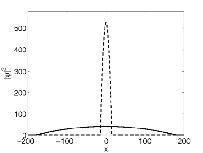
Figure 2: Free expansion of an initially trapped BEC over 5 seconds. Length is measured in harmonic oscillator units. The dashed line shows the density of the BEC at the instant of release, the solid line shows the condensate at the end of the free expansion.

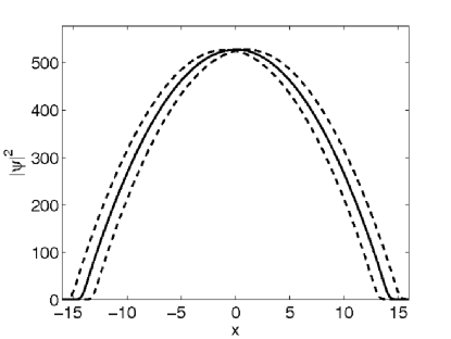
Figure 3: Oscillatory motion of a condensate that is initially displaced by $x_{0}=1\,a_{ho}$ from the equilibrium position. The Kohn mode oscillates with the trap angular frequency $\omega_{z}$ and decouples from the free fall dynamics. The solid line shows the density of the BEC at equilibrium, the dashed lines correspond to the turning points.

IV Many identical atoms within the drop capsule in a rotating frame

In the previous sections, we have deliberately omitted the rotation of the Earth from our discussion in order to simplify the algebra and focus on the essential physics. In particular, we only considered the transformation from the Earth-fixed inertial frame $\{\mathbf{e}_{i}\}$, located at its origin, to the accelerated frame of the freely falling, center-of-mass coordinate ${\bm{\mathcal{R}}}(t)$ of the atomic cloud (see Fig. 1).

IV.1 Classical physics of the drop capsule in a rotating frame of the Earth

IV.1.1 Classification of the three important frames of reference

In fact, in our considerations three different frames of reference are of significant importance. Besides the inertial frame, a real experiment obviously requires a description in a coordinate system that is aligned with the corotating drop tower tube. Moreover, in the frame comoving with the drop capsule, the experiment can be described in a most simple way. In this frame of reference, non-inertial forces can be eliminated. It is of special importance to describe the mapping between the drop tower frame and the capsule frame, since both systems can be used for observation, in principle. In the inertial frame, a point-like particle is characterized by $(\mathbf{r},\mathbf{p})$, and the drop capsule is at position $\bm{\rho}$. In the corotating drop tower frame, with origin at the bottom of the tower, we indicate these quantities with $(\bar{\mathbf{r}}^{\prime},\bar{\mathbf{p}}^{\prime})$ and $\bar{\bm{\rho}}^{\prime}$, while in the drop capsule frame the particle’s coordinate and momentum are $(\mathbf{r}^{\prime\prime},\mathbf{p}^{\prime\prime})$. A schematic sketch of the three systems is depicted in Fig 4.

Figure 4: Schematic view of the three different reference frames as seen from above the North pole. In the inertial frame, located at the center of the Earth, a particle is characterized by $(\mathbf{r},\mathbf{p})$, and the drop capsule is at position $\bm{\rho}$. In the corotating drop tower frame, with the origin at the bottom of the tower, these quantities are denoted by $(\bar{\mathbf{r}}^{\prime},\bar{\mathbf{p}}^{\prime})$ and $\bar{\bm{\rho}}^{\prime}$, while in the drop capsule frame the particle’s coordinate and momentum are $(\mathbf{r}^{\prime\prime},\mathbf{p}^{\prime\prime})$.

IV.1.2 Characterization of the drop tower frame

In the rest frame of the drop tower, the coordinate system is aligned with the rotating tower principal axes denoted by $\{\mathbf{\bar{e}}_{j}(t)\}$. This is depicted in Fig. 5. $\theta$ denotes the angle between the rotational axis of the Earth and the plummet at the geographic location $(\phi,\Theta)$ of the drop tower $\bm{\Re}$. Due to the ellipsoidal shape of the Earth, the plummet does not point to the center of the Earth. The oblateness is modeled by the half axes $a$ and $b$. The instantaneous principal tower axes, as well as the direction towards the base of the tower $\bm{\Re}(t)$

$$\mathbf{\bar{e}}_{i}(t) =M_{\small{\small\earth}}(t)\,M_{\phi\mathbf{e}_{3}}\,M_{\theta\mathbf{e}_{2}}\,\mathbf{e}_{i}, \quad\dot{{\bar{{\bf e}}}}_{i} ={\bm{\Omega}_{{\tiny\earth}}}\times\mathbf{\bar{e}}_{i},$$ (102)

$$\bm{\Re}(t) =M_{\small{\small\earth}}(t)\,M_{\phi\mathbf{e}_{3}}\,M_{\Theta\mathbf{e}_{2}}\,\mathbf{e}_{3}, \quad\dot{\bm{\Re}} ={\bm{\Omega}_{{\tiny\earth}}}\times\bm{\Re},$$ (103)

are obtained from the inertial axes of the Earth $\{\mathbf{e}_{i}\}$ by aligning the $\mathbf{\bar{e}}_{3}$-axis of the tower along the direction of the plummet, followed by a rotation $\phi$ to the longitude of the tower at ZARM/Bremen, as well as the diurnal rotation $M_{\small{\small\earth}}(t)$ around the Earth axis ${\bm{\Omega}_{{\tiny\earth}}}={\Omega_{{\tiny\earth}}}\,\mathbf{e}_{3}$ with an angular frequency ${\Omega_{{\tiny\earth}}}=7.2\times 10^{-5}$ 1/s. No further time-dependence caused by geophysical effects, like tidal forces, precession, or wobbling due to the liquid core motion will be considered.

Now we are in the position to represent all vectors either in the inertial Cartesian basis of the Earth or the corotating frame i. e.,

$$\mathbf{q}(t) =\sum_{i=1}^{3}q^{i}(t)\,\,\mathbf{e}_{i}=\sum_{j=1}^{3}\bar{q}^{j}(t)\,\,\mathbf{\bar{e}}_{j}(t),$$ (104)

$$q_{i} =\sum_{j=1}^{3}\mathbf{e}_{i}\mathbf{\bar{e}}_{j}\,\bar{q}^{j}=\sum_{j=1}^{3}M_{ij}(t)\,\bar{q}^{j},$$ (105)

by introducing the matrix representation of the orthogonal rotation $M(t)^{\top}M(t)=\mathds{1}$ defined by Eq. (102). It is obvious that the components of the Earth rotation as well as the pointer to the base of the tower

$$\bar{\Omega}_{\tiny\earth}^{i} ={\Omega_{{\tiny\earth}}}\,(-\sin\theta,0,\cos\theta),$$ (106)

$$\bar{\Re}^{i} =\Re\,(\sin{(\Theta-\theta)},0,\cos{(\Theta-\theta)}),$$ (107)

must be time independent in this basis.

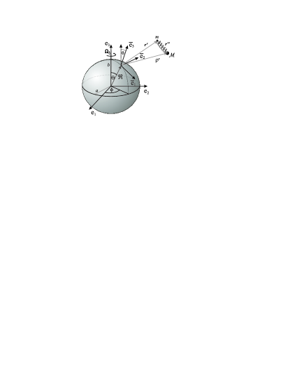
Figure 5: A harmonically trapped particle with position $\mathbf{r}^{\prime}$ and mass $m$ in the drop capsule with position $\bm{\rho}^{\prime}$ and mass $\mathcal{M}$. The position in the capsule frame is denoted by $\mathbf{r}^{\prime\prime}$. The drop tower axes $\{\mathbf{\bar{e}}_{i}\}$ perform a diurnal rotation around the Earth axes ${\bm{\Omega}_{{\tiny\earth}}}$. $\theta$ denotes the angle between the rotational axis of the Earth and the plummet at the geographic location $(\phi,\Theta)$ of the drop tower $\bm{\Re}$. The oblate ellipsoidal shape of the Earth is modeled by the half axes $a$ and $b$.

IV.1.3 Dynamics of the drop capsule

All distances will be measured relative to the base of the drop tower $\bm{\Re}(t)$, i. e.,

$$\bm{\rho}=\bm{\rho}^{\prime}+\bm{\Re}=M(t)\,\bar{\bm{\rho}}=M(t)\,(\bar{\bm{\rho}}^{\prime}+\bar{\bm{\Re}}).$$ (108)

By differentiation, one finds the relation between the velocities with respect to the two frames as

$$\dot{\bm{\rho}} =M(t)\,(\dot{\bar{\bm{\rho}}}^{\prime}+{\bar{\bm{\Omega}}_{{\tiny\earth}}}\times\bar{\bm{\rho}}).$$ (109)

In the rotating frame, the Lagrangian of Eq. (3) for the relative position $\bar{\bm{\rho}}^{\prime}$ as well as the relative velocity $\dot{\bar{\bm{\rho}}}^{\prime}$ reads

$$\begin{gathered}\bar{L}_{c}^{\prime}[\bar{\bm{\rho}}^{\prime},\dot{\bar{\bm{\rho}}}^{\prime},t]=\mathcal{M}\left(\frac{(\dot{\bar{\bm{\rho}}}^{\prime}+{\bar{\bm{\Omega}}_{{\tiny\earth}}}\times\bar{\bm{\rho}})^{2}}{2}-V_{g}(M(t)\bar{\bm{\rho}},t)\right)\\ =\mathcal{M}\left(\frac{\dot{\bar{\bm{\rho}}}^{\prime 2}}{2}-V_{c}(\bar{\bm{\rho}})-V_{g}(M(t)\bar{\bm{\rho}},t)\right)+{\bar{\bm{\Omega}}_{{\tiny\earth}}}(\bar{\bm{\rho}}\times\dot{\bar{\bm{\rho}}}^{\prime}\mathcal{M}).\end{gathered}$$ (110)

Here, we have introduced the centrifugal potential as

$$\bar{v}_{c}^{(2)} ={\bar{\bm{\Omega}}_{{\tiny\earth}}}\otimes{\bar{\bm{\Omega}}_{{\tiny\earth}}}-{{\Omega_{{\tiny\earth}}}^{2}},$$ (111)

$$V_{c}(\bar{\bm{\rho}}) =\frac{1}{2}(\bar{\bm{\rho}}\otimes\bar{\bm{\rho}})\cdot\bar{v}_{c}^{(2)}.$$

The canonical momentum $\bar{\bm{\pi}}^{\prime}$, that is conjugate to the coordinate $\bar{\bm{\rho}}^{\prime}$, is given by

$$\bar{\bm{\pi}}^{\prime}=\frac{\partial\bar{L}_{c}^{\prime}}{\partial\dot{\bar{\bm{\rho}}}^{\prime}}=\mathcal{M}(\dot{\bar{\bm{\rho}}}^{\prime}+{\bar{\bm{\Omega}}_{{\tiny\earth}}}\times\bar{\bm{\rho}})$$ (112)

and implies a Hamiltonian in the new coordinates

$$\begin{split}\bar{H}_{c}^{\prime}(&\bar{\bm{\rho}}^{\prime},\bar{\bm{\pi}}^{\prime})=\bar{\bm{\pi}}^{\prime}\dot{\bar{\bm{\rho}}}^{\prime}-\bar{L}_{c}^{\prime}\\ &=\frac{\bar{\bm{\pi}}^{\prime 2}}{2\mathcal{M}}+\mathcal{M}V_{g}(M(t)\bar{\bm{\rho}},t)-{\bar{\bm{\Omega}}_{{\tiny\earth}}}\bar{\bf{l}}_{c}^{\prime},\end{split}$$ (113)

where the angular momentum $\bar{\bf{l}}_{c}^{\prime}=\bar{\bm{\rho}}\times\bar{\bm{\pi}}^{\prime}$ has been introduced. Via Hamilton’s equations

$$\dot{\bar{\bm{\rho}}}^{\prime} =\frac{\partial\bar{H}_{c}^{\prime}}{\partial\bar{\bm{\pi}}^{\prime}}=\frac{\bar{\bm{\pi}}^{\prime}}{\mathcal{M}}-{\bar{\bm{\Omega}}_{{\tiny\earth}}}\times\bar{\bm{\rho}},$$ (114)

$$\dot{\bar{\bm{\pi}}}^{\prime} =-\frac{\partial\bar{H}_{c}^{\prime}}{\partial\bar{\bm{\rho}}^{\prime}}=-\mathcal{M}\frac{\partial}{\partial\bar{\bm{\rho}}^{\prime}}V_{g}(M(t)\bar{\bm{\rho}},t)-{\bar{\bm{\Omega}}_{{\tiny\earth}}}\times\bar{\bm{\pi}}^{\prime},$$ (115)

we are lead directly to the well-known Newton equations in the rotating frame Greiner (1989)

$$\ddot{\bar{\bm{\rho}}}^{\prime}=-2\,{\bar{\bm{\Omega}}_{{\tiny\earth}}}\times\dot{\bar{\bm{\rho}}}^{\prime}-\frac{\partial}{\partial\bar{\bm{\rho}}^{\prime}}[V_{c}(\bar{\bm{\rho}})+V_{g}(M(t)\bar{\bm{\rho}},t)],$$ (116)

where the first term is the Coriolis force, followed by the centrifugal force of Eq. (111) and the gravitational force as defined before in Eq. (9). By expanding the gravitational potential to second order around the base of the drop tower $\bm{\Re}$ (see Fig. 5), we obtain

$$\ddot{\bar{\bm{\rho}}}^{\prime}=-2\, {\bar{\bm{\Omega}}_{{\tiny\earth}}}\times\dot{\bar{\bm{\rho}}}^{\prime}-\bar{\mathbf{g}}(\bm{\Re})-\left(\bar{v}^{(2)}_{g}(\bm{\Re})+\bar{v}_{c}^{(2)}\right)\,\bar{\bm{\rho}}^{\prime}.$$ (117)

Here, we have introduced the effective gravitational acceleration and rotated Taylor coefficients

$$\bar{\mathbf{g}}(\bm{\Re}) =\bar{\mathbf{v}}^{(1)}_{g}(\bm{\Re})+{\bar{\bm{\Omega}}_{{\tiny\earth}}}\times\left({\bar{\bm{\Omega}}_{{\tiny\earth}}}\times\bar{\bm{\Re}}\right),$$ (118)

$$\bar{\mathbf{v}}^{(1)}_{g}(\bm{\Re}) =M(t)^{\top}\mathbf{v}^{(1)}_{g}(\bm{\Re}),$$ (119)

$$\bar{v}^{(2)}_{g}(\bm{\Re}) =M(t)^{\top}v^{(2)}_{g}(\bm{\Re})M(t),$$ (120)

at the surface of the Earth. $\bar{\mathbf{g}}$ is normal to the surface and takes into account the ellipsoidal shape of the Earth. In order to obtain a simple solution of Eq. (117), one can neglect the centrifugal term, since it is of the order ${\Omega_{{\tiny\earth}}}^{2}\approx 10^{-9}\text{m}/s^{2}$, see Appendix C. An estimate of the Coriolis deviation in $\bar{\mathbf{e}}_{2}$-direction after a drop distance of 100 m yields approximately 2 cm, which is not negligible.

IV.2 A single classical particle in the drop capsule

IV.2.1 Transformation from inertial- to tower coordinates

Now, let us get back to the harmonically trapped particle at $\mathbf{r}$ inside the drop capsule $\bm{\rho}$ and consider its motion with respect to the rotating base of the tower at $\bm{\Re}$ analogous to Eq. (19). In this case, coordinates and velocities are given by

$$\mathbf{r} =M(t)\bar{\mathbf{r}}=M(t)(\bar{\mathbf{r}}^{\prime}+\bar{\bm{\Re}}),$$ (121)

$$\dot{\mathbf{r}} =M(t)\,(\dot{\bar{\mathbf{r}}}^{\prime}+{\bar{\bm{\Omega}}_{{\tiny\earth}}}\times\bar{\mathbf{r}}).$$ (122)

Note, that this description refers to the tower coordinates.

The trap rests in the drop capsule, which is moving on the classical trajectory given by Eq. (116). From the Lagrangian in the inertial frame, Eq. (13), we obtain the Lagrangian for the particle coordinates relative to the base of the drop tower

$$\bar{L}^{\prime}_{sp}[ \bar{\mathbf{r}}^{\prime},\dot{\bar{\mathbf{r}}}^{\prime},t]=m\Big{[}\frac{1}{2}(\dot{\bar{\mathbf{r}}}^{\prime}+{\bar{\bm{\Omega}}_{{\tiny\earth}}}\times\bar{\mathbf{r}})^{2}$$ (123)

$$-V_{t}(M(t)(\bar{\mathbf{r}}^{\prime}-\bar{\bm{\rho}}^{\prime}),t)-V_{g}(M(t)(\bar{\mathbf{r}}^{\prime}+\bar{\bm{\Re}}),t)\Big{]}.$$

The total Lagrangian, which includes the Lagrangians both of the drop capsule as well as the single trapped particle, reads

$$\bar{L}^{\prime}=\bar{L}_{c}^{\prime}+\bar{L}_{sp}^{\prime}$$ (124)

with $\bar{L}_{c}^{\prime}$ as defined in Eq. (110). The linear canonical momentum is

$$\bar{\mathbf{p}}^{\prime} =\frac{\partial\bar{L}_{sp}}{\partial\dot{\bar{\mathbf{r}}}^{\prime}}=m\,(\dot{\bar{\mathbf{r}}}^{\prime}+{\bar{\bm{\Omega}}_{{\tiny\earth}}}\times\bar{\mathbf{r}}),$$ (125)

and thus one finds for the Hamiltonian

$$\bar{H}_{sp}^{\prime}( \bar{\mathbf{r}}^{\prime},\bar{\mathbf{p}}^{\prime},t)=\frac{\bar{\mathbf{p}}^{\prime 2}}{2m}+V_{t}(M(t)(\bar{\mathbf{r}}^{\prime}-\bar{\bm{\rho}}^{\prime}),t)$$

$$+V_{g}(M(t)(\bar{\mathbf{r}}^{\prime}+\bar{\bm{\Re}}),t)-\bar{\mathbf{p}}^{\prime}\left({\bar{\bm{\Omega}}_{{\tiny\earth}}}\times\bar{\mathbf{r}}\right).$$ (126)

Then Hamilton’s equations of motion read

$$\dot{\bar{\mathbf{r}}}^{\prime}=\frac{\partial\bar{H}_{sp}^{\prime}}{\partial\bar{\mathbf{p}}^{\prime}}=\frac{\bar{\mathbf{p}}^{\prime}}{m}-{\bar{\bm{\Omega}}_{{\tiny\earth}}}\times\bar{\mathbf{r}},$$ (127)

$$\dot{\bar{\mathbf{p}}}^{\prime}=-\frac{\partial\bar{H}_{sp}^{\prime}}{\partial\bar{\mathbf{r}}^{\prime}}=-\frac{\partial}{\partial\bar{\mathbf{r}}^{\prime}}\left(V_{t}+V_{g}\right)+\bar{\mathbf{p}}^{\prime}\times{\bar{\bm{\Omega}}_{{\tiny\earth}}},$$ (128)

correspondingly. Finally, Newton’s equation is given by

$$\begin{split}\ddot{\bar{\mathbf{r}}}^{\prime}=&-\frac{\partial}{\partial\bar{\mathbf{r}}^{\prime}}\left(V_{t}(M(t)(\bar{\mathbf{r}}^{\prime}-\bar{\bm{\rho}}^{\prime}),t)+V_{g}(M(t)(\bar{\mathbf{r}}^{\prime}+\bar{\bm{\Re}}),t)\right)\\ &-{\bar{\bm{\Omega}}_{{\tiny\earth}}}\times({\bar{\bm{\Omega}}_{{\tiny\earth}}}\times\bar{\mathbf{r}})-2{\bar{\bm{\Omega}}_{{\tiny\earth}}}\times\dot{\bar{\mathbf{r}}}^{\prime}.\end{split}$$ (129)

If we expand the gravitational potential up to second order, we obtain

$$\ddot{\bar{\mathbf{r}}}^{\prime}= -2\,{\bar{\bm{\Omega}}_{{\tiny\earth}}}\times\dot{\bar{\mathbf{r}}}^{\prime}-\bar{\mathbf{g}}(\bar{\bm{\rho}})-\frac{\partial}{\partial\bar{\mathbf{r}}^{\prime}}\check{\bar{V}}_{t}(\bar{\mathbf{r}}^{\prime}-\bar{\bm{\rho}}^{\prime},\bar{\bm{\rho}},t)$$

$$= -2\,{\bar{\bm{\Omega}}_{{\tiny\earth}}}\times\dot{\bar{\mathbf{r}}}^{\prime}-\check{\bar{v}}^{(2)}(\bar{\bm{\rho}},t)\,(\bar{\mathbf{r}}^{\prime}-\bar{\mathbf{r}}^{\prime}_{eq}(t)).$$ (130)

As in the non-rotating situation of Sec. II.2.3, we get an equilibrium position $\bar{\mathbf{r}}^{\prime}_{eq}(t)$, which is defined by

$$\check{\bar{v}}^{(2)}(\bar{\bm{\rho}},t)\,\bar{\mathbf{r}}^{\prime}_{eq}(t)=-\bar{\mathbf{g}}(\bar{\bm{\rho}})+\check{\bar{v}}^{(2)}(\bar{\bm{\rho}},t)\bar{\bm{\rho}}^{\prime}$$ (131)

and a modified, appropriately rotated harmonic trapping potential

$$\check{\bar{v}}^{(2)}(\bar{\bm{\rho}},t)=\bar{v}_{t}^{(2)}(t)+\bar{v}^{(2)}_{g}(\bar{\bm{\rho}},t)+\bar{v}_{c}^{(2)},$$ (132)

$$\bar{v}^{(2)}_{t}(t)=M(t)^{\top}\,v^{(2)}_{t}(t)\,M(t),$$ (133)

$$\check{\bar{V}}_{t}({\bm{\xi}},\bar{\bm{\rho}},t)=\frac{1}{2}\,({\bm{\xi}}\otimes{\bm{\xi}})\cdot\check{\bar{v}}^{(2)}(\bar{\bm{\rho}},t).$$ (134)

The equilibrium position $\bar{\mathbf{r}}^{\prime}_{eq}(t)$ is governed by the trajectory of the drop capsule $\bar{\bm{\rho}}^{\prime}$, however there is a gravitational sag.

IV.2.2 Hamiltonian formulation of the canonical transformation from tower- to capsule coordinates

In order to obtain the classical Hamiltonian of a single trapped particle in capsule coordinates, we introduce the canonical transformation

$$G(\bar{\mathbf{r}}^{\prime},{\mathbf{p}}^{\prime\prime},t)=\left[M\left(\bar{\mathbf{r}}^{\prime}-\bar{\bm{\rho}}^{\prime}(t)\right)\right]{\mathbf{p}}^{\prime\prime}+\frac{m}{\mathcal{M}}\left[\bar{s}^{\prime}(t)+\bar{\mathbf{r}}^{\prime}\bm{\bar{\pi}}^{\prime}(t)\right],$$ (135)

which yields

$$\mathbf{r}^{\prime\prime}=\frac{\partial G}{\partial{\mathbf{p}}^{\prime\prime}}=M\left(\bar{\mathbf{r}}^{\prime}-\bar{\bm{\rho}}^{\prime}(t)\right),$$ (136)

$$\bar{\mathbf{p}}^{\prime}=\frac{\partial G}{\partial\bar{\mathbf{r}}^{\prime}}=M^{\top}(t){\mathbf{p}}^{\prime\prime}+\frac{m}{\mathcal{M}}\bm{\bar{\pi}}^{\prime}(t).$$ (137)

In this particular gauge, the one-particle Hamiltonian is given by

$$H_{sp}^{\prime\prime} (\mathbf{r}^{\prime\prime},{\mathbf{p}}^{\prime\prime},t)=\bar{H}_{sp}^{\prime}(\bar{\mathbf{r}}^{\prime},\bar{\mathbf{p}}^{\prime},t)+\frac{\partial}{\partial t}G(\bar{\mathbf{r}}^{\prime},{\mathbf{p}}^{\prime\prime},t)$$ (138)

$$= \frac{{\mathbf{p}}^{\prime\prime 2}}{2\,m}+m\widetilde{V}_{t}(\mathbf{r}^{\prime\prime},\bm{\rho},t).$$

provided the equations for the capsule, Eqs. (114) and (115), are satisfied and $\bar{s}^{\prime}(t,t_{0})$ is an action,

$$\bar{s}^{\prime}(t,t_{0})=\int_{t_{0}}^{t}dt^{\prime}\bar{L}_{c}^{\prime}[\bar{\bm{\rho}}^{\prime},\dot{\bar{\bm{\rho}}}^{\prime},t^{\prime}]-\bar{\bm{\rho}}^{\prime}\,\bm{\bar{\pi}}^{\prime}|^{t}_{t_{0}}.$$ (139)

Obviously, this Hamiltonian is identical to Eq. (36).

IV.3 Many identical atoms in the drop-capsule

IV.3.1 Frame transformations between tower- and capsule coordinates

The calculations of Sec. III excluded the effects of rotation. In here, we will rectify this and obtain a general frame transformation that eliminates external forces and torques from Schrödinger’s equation. In particular, this is applied to the problem of gravitational acceleration and Earth’s rotation.

We have already introduced the generic many-particle Hamiltonian with translationally invariant, binary interactions in Eq. (48). However, we have not exploited the fact that only the s-partial wave contributes to the two-particle scattering at low energies. Thus, we want to assume that the relative angular momentum is a good quantum number. This can be modeled by an interatomic potential that is only a function of the relative distance, $V_{p}(|{\bm{\xi}}|)$. In the case of fermionic particles, this means there is no s-wave interaction due to the Pauli exclusion principle and the gas becomes ideal at low energies.

Let us start with the full many-particle Hamiltonian

$$\hat{\bar{H}}^{\prime}=\hat{\bar{H}}^{\prime}_{sp}(t)+\hat{\bar{V}}^{\prime}_{p},$$ (140)

$$\hat{\bar{V}}^{\prime}_{p}=\frac{1}{2}\int\,\text{d}^{6}\bar{r}^{\prime}{\hat{a}^{{\dagger}}(\bar{\mathbf{r}}^{\prime}_{1})}{\hat{a}^{{\dagger}}(\bar{\mathbf{r}}^{\prime}_{2})}\bar{V}^{\prime}_{p}(|\bar{\mathbf{r}}^{\prime}_{1}-\bar{\mathbf{r}}^{\prime}_{2}|){\hat{a}^{\vphantom{{\dagger}}}(\bar{\mathbf{r}}^{\prime}_{2})}{\hat{a}^{\vphantom{{\dagger}}}(\bar{\mathbf{r}}^{\prime}_{1})}$$

in the drop tower frame.

Now, we have to transform the Schrödinger state from the drop tower frame, $\left|\Psi(t)\right\rangle$, to the rest frame of the drop capsule, $\left|\Psi(t)\right\rangle={\hat{U}^{\vphantom{\dagger}}}(t)\left|\Psi(t)\right\rangle^{\prime}$. This requires to augment the unitary frame transformation from Eq. (71) of Sec. III.3,

$${\hat{U}^{\vphantom{\dagger}}}(t)=\hat{U}_{\bar{\mathcal{S}^{\prime}}(t)}\,\hat{U}_{\bar{\mathcal{P}^{\prime}}(t)}\,\hat{U}_{\bar{\mathcal{R}^{\prime}}(t)}\,\hat{U}^{\dagger}_{M(t)},$$ (141)

with

$$\hat{U}_{M(t)}=e^{-i/\hbar\,{\bm{\mathcal{Q}}}(t){\hat{\mathbf{L}}}}\,e^{-i/\hbar\,\phi\,\mathbf{e}_{3}{\hat{\mathbf{L}}}}\,e^{-i/\hbar\,\theta\mathbf{e}_{2}{\hat{\mathbf{L}}}}.$$ (142)

In there, we performed the same rotations as in Eq. (102), and in particular, the diurnal rotation around the Earth axis, ${\bm{\mathcal{Q}}}(t)={\bm{\Omega}_{{\tiny\earth}}}\,t$, is accounted for. Moreover, we would like to point out again that we transform from the drop tower frame, which is corotating with the Earth, to the instantaneous rest frame of the drop capsule, which is not rotating. Therefore we need to apply $\hat{U}^{\dagger}_{M(t)}$ rather than $\hat{U}_{M(t)}$.

The transformation rule for the Hamilton operator was given in Eq. (73) and consists of three contributions. The first one contains merely the gauge contributions that arise from the time-dependent frame parameters

$${\hat{U}^{\dagger}}(t)(-i\hbar\frac{d}{dt}){\hat{U}^{\vphantom{\dagger}}}(t)= (\dot{\bar{{\mathcal{S}}}}^{\prime}+\dot{\bar{{\bm{\mathcal{P}}}}}^{\prime}\,\bar{{\bm{\mathcal{R}}}}^{\prime})\,{\hat{N}}+\dot{\bar{{\bm{\mathcal{P}}}}}^{\prime}(M^{\top}{\hat{\mathbf{R}}})$$ (143)

$$-\dot{\bar{{\bm{\mathcal{R}}}}}^{\prime}(M^{\top}{\hat{\mathbf{P}}})+{\bm{\Omega}_{{\tiny\earth}}}\,{\hat{\mathbf{L}}}.$$

For obtaining this result, we have used the basic Eqs. (44), (193) and (194). The second contribution is the transformed single-particle Hamiltonian

$$\begin{gathered}{\hat{U}^{\dagger}}(t)\,\hat{\bar{H}}^{\prime}_{sp}(t)\,{\hat{U}^{\vphantom{\dagger}}}(t)=\\ \int\text{d}^{3}r^{\prime\prime}\,{\hat{a}^{{\dagger}}(\mathbf{r}^{\prime\prime})}\bar{H}^{\prime}_{sp}(M^{\top}\mathbf{r}^{\prime\prime}+\bar{{\bm{\mathcal{R}}}}^{\prime},M^{\top}{\mathbf{p}}^{\prime\prime}+\bar{{\bm{\mathcal{P}}}}^{\prime},t){\hat{a}^{\vphantom{{\dagger}}}(\mathbf{r}^{\prime\prime})}.\end{gathered}$$ (144)

Finally, the third contribution is simply the transformed binary interaction potential.

$${\hat{U}^{\dagger}}(t)\,\hat{\bar{V}}^{\prime}_{p}\,{\hat{U}^{\vphantom{\dagger}}}(t)=\hat{\bar{V}}^{\prime}_{p}\equiv\hat{V}_{p}.$$ (145)

It is left unchanged due to particle conservation, the local character of the potential, as well as the translational and rotational invariance, i. e.,

$$[{\hat{N}},\hat{V}_{p}]=[{\hat{\mathbf{R}}},\hat{V}_{p}]=[{\hat{\mathbf{P}}},\hat{V}_{p}]=[{\hat{\mathbf{L}}},\hat{V}_{p}]=0.$$ (146)

Combining these results, we find the transformed Hamiltonian in the accelerated and non-rotating frame as

$$\hat{H}^{\prime\prime}(t)=\int\,\text{d}^{3}r^{\prime\prime}\,{\hat{a}^{{\dagger}}(\mathbf{r}^{\prime\prime})}\,H^{\prime\prime}_{sp}(\mathbf{r}^{\prime\prime},{\mathbf{p}}^{\prime\prime},t)\,{\hat{a}^{\vphantom{{\dagger}}}(\mathbf{r}^{\prime\prime})}+\hat{V}_{p}.$$ (147)

All gauge contributions are contained in the definition of the modified single-particle Hamiltonian

$$\begin{split}H^{\prime\prime}_{sp}(&\mathbf{r}^{\prime\prime},{\mathbf{p}}^{\prime\prime},t)=\bar{H}_{sp}^{\prime}(M^{\top}\mathbf{r}^{\prime\prime}+\bar{{\bm{\mathcal{R}}}}^{\prime},M^{\top}{\mathbf{p}}^{\prime\prime}+\bar{{\bm{\mathcal{P}}}}^{\prime},t)\\ &+\dot{\bar{{\mathcal{S}}}}^{\prime}+\dot{\bar{{\bm{\mathcal{P}}}}}^{\prime}\,\bar{{\bm{\mathcal{R}}}}^{\prime}+\dot{\bar{{\bm{\mathcal{P}}}}}^{\prime}\,(M^{\top}\mathbf{r}^{\prime\prime})-\dot{\bar{{\bm{\mathcal{R}}}}}^{\prime}\,(M^{\top}{\mathbf{p}}^{\prime\prime})\\ &+{\mathbf{p}}^{\prime\prime}\left({\bm{\Omega}_{{\tiny\earth}}}\times\mathbf{r}^{\prime\prime}\right).\end{split}$$ (148)

IV.3.2 Application of the frame transformation to the many-particle Hamiltonian in harmonic approximation

We will now apply the considerations of the previous subsection to the falling trapped interacting many-particle system in the rotating frame. The single-particle Hamilton operator follows from the classical considerations of Eq. (IV.2.1) and is given by

$$\bar{H}_{sp}^{\prime}( \bar{\mathbf{r}}^{\prime},\bar{\mathbf{p}}^{\prime},t)=\frac{\bar{\mathbf{p}}^{\prime 2}}{2m}+V_{t}(M(t)(\bar{\mathbf{r}}^{\prime}-\bar{\bm{\rho}}^{\prime}),t)$$

$$+V_{g}(M(t)(\bar{\mathbf{r}}^{\prime}+\bar{\bm{\Re}}),t)-\bar{\mathbf{p}}^{\prime}\left({\bar{\bm{\Omega}}_{{\tiny\earth}}}\times\bar{\mathbf{r}}\right).$$ (149)

By splitting the transformed Hamiltonian from Eq. (148) into constant, linear and higher order polynomial contributions in terms of the position $\bar{\mathbf{r}}^{\prime}$ and the momentum $\bar{\mathbf{p}}^{\prime}$, one finds

$$\begin{split}H^{\prime\prime}_{sp}(\mathbf{r}^{\prime\prime},{\mathbf{p}}^{\prime\prime},t)=&\left[\bm{\alpha}\left(M^{\top}{\mathbf{p}}^{\prime\prime}\right)+\bm{\beta}\left(M^{\top}\mathbf{r}^{\prime\prime}\right)+\gamma\right]\\ &+\frac{{\mathbf{p}}^{\prime\prime 2}}{2m}+m\widetilde{V}_{{t}}\left(\mathbf{r}^{\prime\prime},M\bar{{\bm{\mathcal{R}}}}^{\prime}+\bm{\Re},t\right).\end{split}$$ (150)

In there, we neglected terms of third and higher order in the gravitational potential. The coefficients read

$$\bm{\alpha}= \frac{\bar{{\bm{\mathcal{P}}}}^{\prime}}{m}-\dot{\bar{{\bm{\mathcal{R}}}}}^{\prime}-{\bar{\bm{\Omega}}_{{\tiny\earth}}}\times\left(\bar{{\bm{\mathcal{R}}}}^{\prime}+\bar{\bm{\Re}}\right),$$ (151)

$$\begin{split}\bm{\beta}=&\dot{\bar{{\bm{\mathcal{P}}}}}^{\prime}-\bar{{\bm{\mathcal{P}}}}^{\prime}\times{\bar{\bm{\Omega}}_{{\tiny\earth}}}\\ &+m\,\frac{\partial}{\partial\bar{{\bm{\mathcal{R}}}}^{\prime}}[V_{t}(M(\bar{{\bm{\mathcal{R}}}}^{\prime}-\bar{\bm{\rho}}^{\prime}),t)+V_{g}(M(\bar{{\bm{\mathcal{R}}}}^{\prime}+\bar{\bm{\Re}}),t)].\end{split}$$ (152)

and

$$\gamma=\dot{\bar{{\mathcal{S}}}}^{\prime}-\left[\bar{L}^{\prime}_{sp}(\bar{{\bm{\mathcal{R}}}}^{\prime},\dot{\bar{{\bm{\mathcal{R}}}}}^{\prime},t)-\frac{d}{dt}\left(\bar{{\bm{\mathcal{P}}}}^{\prime}\bar{{\bm{\mathcal{R}}}}^{\prime}\right)\right].$$ (153)

If the constraints are satisfied identically, i. e., $\{\bm{\alpha},\bm{\beta},\gamma\}\rightarrow 0$, one obtains the single-particle Hamiltonian in the accelerated frame,

$$\begin{aligned} H_{sp}^{\prime\prime}(\mathbf{r}^{\prime\prime},{\mathbf{p}}^{\prime\prime},t)=&\frac{{\mathbf{p}}^{\prime\prime 2}}{2\,m}+m\,\widetilde{V}_{{t}}\left(\mathbf{r}^{\prime\prime},M\bar{{\bm{\mathcal{R}}}}^{\prime}+\bm{\Re},t\right),\end{aligned}$$ (154)

provided the frame parameters as well as the center-of-mass of the drop capsule $\{\bar{{\bm{\mathcal{R}}}}^{\prime}(t),\bar{{\bm{\mathcal{P}}}}^{\prime}(t),\bar{\bm{\rho}}^{\prime}(t)\}$ satisfy the classical equations of motion

$$\bar{\bm{\pi}}^{\prime}=\frac{\partial\bar{L}_{c}^{\prime}}{\partial\dot{\bar{\bm{\rho}}}^{\prime}}=\mathcal{M}\left(\dot{\bar{\bm{\rho}}}^{\prime}+{\bar{\bm{\Omega}}_{{\tiny\earth}}}\times\bar{\bm{\rho}}\right),\quad\dot{\bar{\bm{\pi}}}^{\prime}=\frac{\partial\bar{L}_{c}^{\prime}}{\partial\bar{\bm{\rho}}^{\prime}},$$ (155)

$$\bar{{\bm{\mathcal{P}}}}^{\prime}=\frac{\partial\bar{L}_{sp}^{\prime}}{\partial\dot{\bar{{\bm{\mathcal{R}}}}}^{\prime}}=m\left(\dot{\bar{{\bm{\mathcal{R}}}}}^{\prime}+{\bar{\bm{\Omega}}_{{\tiny\earth}}}\times(\bar{{\bm{\mathcal{R}}}}^{\prime}+\bar{\bm{\Re}})\right),\quad\dot{\bar{{\bm{\mathcal{P}}}}}^{\prime}=\frac{\partial\bar{L}_{sp}^{\prime}}{\partial\bar{{\bm{\mathcal{R}}}}^{\prime}}.$$ (156)

With Eqs. (155) and (156), we have recovered the Lagrangian $L^{\prime}[\bar{\bm{\rho}}^{\prime},\dot{\bar{\bm{\rho}}}^{\prime},\bar{{\bm{\mathcal{R}}}}^{\prime},\dot{\bar{{\bm{\mathcal{R}}}}}^{\prime},t]$ of Eq. (124), and one can express the accrued dynamical phase as an action integral

$$\bar{{\mathcal{S}}}^{\prime}(t,t_{0})=\int_{t_{0}}^{t}dt^{\prime}\bar{L}_{sp}^{\prime}[\bar{{\bm{\mathcal{R}}}}^{\prime},\dot{\bar{{\bm{\mathcal{R}}}}}^{\prime},t^{\prime}]-\bar{{\bm{\mathcal{P}}}}^{\prime}\bar{{\bm{\mathcal{R}}}}^{\prime}|^{t}_{t_{0}}.$$ (157)

V Two-component atomic gas

Let us now consider identical atoms with two internal electronic degrees of freedom. In this section, we would like to demonstrate that the dynamics of these internal states decouples from the external motion of the trapped falling ultra-cold quantum gas, even in case of binary collisions, if the self-scattering and the cross-component scattering properties are identical.

V.1 Description in second quantization

Henceforth, the inclusion of two degrees of freedom for the inner states in the definition of the field operators is required. These operators are denoted by $\hat{a}_{\mu}(\mathbf{r})$, $\mu\in\{1,2\}$, and satisfy the commutation relation

$$[\hat{a}_{\mu}(\mathbf{r}_{1}),\hat{a}^{\dagger}_{\nu}(\mathbf{\mathbf{r}}_{2})]_{\mp}=\delta_{\mu\nu}\,\delta(\mathbf{r}_{1}-\mathbf{r}_{2}).$$ (158)

The pair potential $\hat{V}_{p}$, which is assumed to be local and exhibits translational and rotational invariance, can be written as Merzbacher (1970)

$$\begin{split}\hat{V}_{p}=&\frac{1}{2}\int\text{d}^{6}r\sum_{\mu_{1}..\mu_{4}=1}^{2}\,V_{p}^{\mu_{1}\mu_{2}\mu_{3}\mu_{4}}(|\mathbf{r}_{1}-\mathbf{r}_{2}|)\\ &\phantom{\frac{1}{2}\int}\hat{a}_{\mu_{1}}^{\dagger}(\mathbf{r}_{1})\,\hat{a}_{\mu_{2}}^{\dagger}(\mathbf{r}_{2})\,\hat{a}_{\mu_{3}}(\mathbf{r}_{2})\,\hat{a}_{\mu_{4}}(\mathbf{r}_{1}).\end{split}$$ (159)

The elements of $V_{p}^{\mu_{1}\mu_{2}\mu_{3}\mu_{4}}$ are linked to the self-species and cross-component scattering lengths of the atom in the different states. In ⁸⁷Rb these quantities are – to a good approximation – all equal, with a deviation of 3-4$\%$ Matthews et al. (1999), so we can neglect the higher multipole contributions beyond the monopole (J=0) term $V_{p}^{\mu_{1}\mu_{2}\mu_{3}\mu_{4}}\approx\delta_{\mu_{1}\mu_{3}}\delta_{\mu_{2}\mu_{4}}\delta_{\mu_{1}\mu_{2}}V_{p}^{(J=0)}$. This leaves us with writing $\hat{V}_{p}$ approximately as

$$\begin{split}\hat{V}_{p}&=\frac{1}{2}\int\text{d}^{6}r\sum_{\mu,\nu}\hat{a}_{\mu}^{\dagger}(\mathbf{r}_{1})\,\hat{a}_{\nu}^{\dagger}(\mathbf{r}_{2})\,V_{p}^{(0)}(|\mathbf{r}_{1}-\mathbf{r}_{2}|)\,\hat{a}_{\nu}(\mathbf{r}_{2})\,\hat{a}_{\mu}(\mathbf{r}_{1})\\ &=\frac{1}{2}\int\text{d}^{6}r\,\hat{n}(\mathbf{r}_{1})(\hat{n}(\mathbf{r}_{2})-\delta(\mathbf{r}_{1}-\mathbf{r}_{2}))\,V_{p}^{(0)}(|\mathbf{r}_{1}-\mathbf{r}_{2}|).\end{split}$$ (160)

We made use of Eq. (158), and introduced the total particle density

$$\hat{n}(\mathbf{r})\equiv\sum_{\mu=1}^{2}\hat{a}_{\mu}^{\dagger}(\mathbf{r})\,\hat{a}_{\mu}^{\phantom{\dagger}}(\mathbf{r}).$$ (161)

We would like to point out that due to our assumptions $\hat{V}_{p}$ is now SU(2) invariant Kuklov and Birman (2000).

The two internal states can be coupled by a classical, traveling-wave laser field via electric dipole interaction Schleich (2001). The strength of the coupling is determined by the Rabi frequency $\Omega(t)$, which may be time-dependent if the laser is pulsed. $\Delta(t)$ denotes the, possibly time-dependent, detuning of the laser with respect to the resonant transition between the two levels. We want to consider large detunings in order to neglect any mechanical recoil effects of the laser on the atoms and, as usual, we have switched to an interaction picture oscillating with the laser frequency Schleich (2001).

In order to describe the dipole interaction of identical particles in the language of second quantization, we introduce the operators

$$\hat{S}_{i}=\sum_{\mu,\nu=1}^{2}\,\int\text{d}^{3}r\,\hat{a}_{\mu}^{\dagger}(\mathbf{r})\,s^{(i)}_{\mu\nu}\,\hat{a}_{\nu}(\mathbf{r})$$ (162)

with the well-known spin-1/2-matrices $s^{(i)}$, $i\in\{1,2,3\}$, Appendix B. Explicitly, the operators read

$$\hat{S}_{1} =\frac{\hbar}{2}\int\text{d}^{3}r\left[\hat{a}_{2}^{\dagger}(\mathbf{r})\hat{a}_{1}^{\phantom{\dagger}}(\mathbf{r})+\hat{a}_{1}^{\dagger}(\mathbf{r})\hat{a}_{2}^{\phantom{\dagger}}(\mathbf{r})\right],$$ (163)

$$\hat{S}_{2} =i\frac{\hbar}{2}\int\text{d}^{3}r\left[\hat{a}_{2}^{\dagger}(\mathbf{r})\hat{a}_{1}^{\phantom{\dagger}}(\mathbf{r})-\hat{a}_{1}^{\dagger}(\mathbf{r})\hat{a}_{2}^{\phantom{\dagger}}(\mathbf{r})\right],$$ (164)

$$\hat{S}_{3} =\frac{\hbar}{2}\int\text{d}^{3}r\left[\hat{a}_{1}^{\dagger}(\mathbf{r})\hat{a}_{1}^{\phantom{\dagger}}(\mathbf{r})-\hat{a}_{2}^{\dagger}(\mathbf{r})\hat{a}_{2}^{\phantom{\dagger}}(\mathbf{r})\right].$$ (165)

These operators fulfill the commutation relations of the angular momentum operators for spin-1/2-particles and therefore represent the SU(2) symmetry. In other words, the properties of the Pauli matrices translate to the picture of the second quantization. Clearly, the angular momentum algebra

$$\left[\hat{S}_{i},\hat{S}_{j}\right]=i\varepsilon_{ijk}\hat{S}_{k}$$ (166)

holds. All the operators $\mathbf{\hat{R}}$, $\mathbf{\hat{P}}$ and $\mathbf{\hat{L}}$ commute with $\hat{S_{i}}$, i.e.

$$\left[\hat{S}_{i},\hat{N}\right]=\left[\hat{S}_{i},\mathbf{\hat{R}}\right]=\left[\hat{S}_{i},\mathbf{\hat{P}}\right]=\left[\hat{S}_{i},\mathbf{\hat{L}}\right]=0.$$ (167)

Please note, that the definition of operators $\mathbf{\hat{N}}$, $\mathbf{\hat{R}}$, $\mathbf{\hat{P}}$, and $\mathbf{\hat{L}}$ has to be modified, taking into account the two different internal states, i.e.

$$\hat{A}=\sum_{\mu=1,2}\int\text{d}^{3}r\,\hat{a}_{\mu}^{\dagger}(\mathbf{r})\,A\,\hat{a}_{\mu}(\mathbf{r}),$$ (168)

where $\hat{A}\in\{\hat{N},\hat{\mathbf{R}},\hat{\mathbf{P}},\hat{\mathbf{L}}\}$, and $A\in\{1,\mathbf{r},\mathbf{p},\mathbf{r}\times\mathbf{p}\}$.

We are now able to write down the full many-body Hamiltonian, containing the one-particle, external dynamics ($\hat{H}_{sp}$), the one-particle internal two-level dynamics ($\hat{V}_{d}$), describing the interaction between matter and light, and the two-particle collisions ($\hat{V}_{p}$),

$$\hat{H}=(\hat{H}_{sp}+\hat{V}_{d})+\hat{V}_{p}.$$ (169)

In there,

$$\hat{H}_{sp}=\sum_{\mu=1,2}\,\int\text{d}^{3}r\,\hat{a}^{\dagger}_{\mu}(\mathbf{r})\,H_{sp}\,\hat{a}_{\mu}(\mathbf{r}).$$ (170)

$H_{sp}$ can be chosen as in Eq. (IV.2.1). $\hat{V}_{d}$ is given by

$$\hat{V}_{d}=\hat{V}_{d}(t)=\Omega(t)\hat{S}_{1}+\Delta(t)\hat{S}_{3}.$$ (171)

V.2 Separation of two-level dynamics and center-of-mass motion

The dynamics of the many-particle system is determined by the Schrödinger equation

$$i\hbar\partial_{t}\left|\Psi(t)\right\rangle=\hat{H}\,\left|\Psi(t)\right\rangle$$ (172)

with $\hat{H}$ from Eq. (169). As we have seen in the preceeding sections, a more efficient description of the dynamics can be obtained by performing a frame transformation. In the present case, we have to account for both external and internal dynamics. Therefore, it would be favorable to separate both types of motion from each other. We choose

$$\left|\Psi(t)\right\rangle=\hat{U}_{d}\,\hat{U}_{\bar{\mathcal{S}}^{\prime}(t)}\,\hat{U}_{\bar{\mathcal{P}}^{\prime}(t)}\,\hat{U}_{\bar{\mathcal{R}}^{\prime}(t)}\,\hat{U}_{M(t)}^{\dagger}\left|\Psi(t)\right\rangle^{\prime},$$ (173)

cf. Eq. (141), and

$$\hat{U}_{d}=\mathcal{T}\,\left\{\,\exp\left[-\frac{i}{\hbar}\,\int_{t_{0}}^{t}\,dt^{\prime}\,\hat{V}_{d}(t^{\prime})\right]\right\},$$ (174)

where $\mathcal{T}$ guarantees time ordering. The latter transformation formally eliminates the two-level dynamics, since it cancels the contribution $\hat{V}_{d}$. The decoupling of the transformation $\hat{U}_{d}$ from the remaining frame transformation results from the fact that

$$\left[\hat{V}_{d},\hat{H}_{sp}+\hat{V}_{p}\right]=0$$ (175)

due to Eq. (167) as well as the SU(2)-invariance of $\hat{V_{p}}$, cf. preceeding subsection. In principle, the propagator $\hat{U}_{d}$ can be determined from the two linearly independent solutions of the time-dependent Rabi problem Allen and Eberly (1987); Barata and Wreszinski (2000); Bagrov et al. (2001).

VI Conclusions

We have described the dynamics of an ultra-cold quantum gas in a long distance free-fall experiment. Starting from the classical mechanics of the drop capsule and a single trapped particle, we developed the quantum-field theoretical description of a trapped, interacting degenerate quantum gas in a drop experiment in an inertial frame, the corotating frame of the Earth and the comoving frame of the drop capsule. By introducing suitable coordinate transformations, it was possible to eliminate non-inertial forces and to focus on effects that take place on the mesoscopic length scale of the Bose or Fermi gas. The exact cancellation of non-inertial forces requires translational invariance, the isotropy of the binary collisional potential and the presence of a quadratic single-particle Hamiltonian. This is well satisfied for ⁸⁷Rb, and the harmonic approximation of the gravitational potential around the center-of mass of the BEC wave-packet is an excellent assumption. Corrections to it could be easily calculated perturbatively.

If the atoms are two-level systems and coupled by an off-resonant traveling-wave laser field, this internal dynamics can be separated from the external motion, provided all scattering lengths are identical (SU(2)-invariance).

This formalism provides us with an efficient way to describe free-fall experiments, especially for numerical studies. It almost goes without saying that it is in particular valid and useful on the mean-field level.

While we have discussed the Euclidean transformations corresponding to translation and rotation, we have omitted the scaling transformations L.Pitaevskii and Rosch (1997), which are obviously very useful to model the adiabatic expansion of a BEC from a trap Castin and Dum (1996). The consideration of the complete set of generalized canonical transformations in a time-dependent way will ultimately separate all ”trivial” dynamics, including wave-packet spreading, from the essential many-particle physics. This is work in progress. We have also not touched questions of relativity. This was done by intention in order to clarify all non-relativistic effects first, which by themselves are highly nontrivial and presumably dominant.

Appendix A Taylor expansion of the gravitational potential

The Taylor expansion of the gravitational potential

$$\begin{gathered}V_{g}(\mathbf{r^{\prime}}+\bm{\rho},t)=[1+\mathbf{r^{\prime}}\,\frac{\partial}{\partial\bm{\rho}}+\frac{1}{2!}(\mathbf{r^{\prime}}\,\frac{\partial}{\partial\bm{\rho}})^{2}+\ldots]\,V_{g}(\bm{\rho},t)\\ =V_{g}(\bm{\rho},t)+V_{g}^{(1)}(\mathbf{r}^{\prime},\bm{\rho},t)+V_{g}^{(2)}(\mathbf{r}^{\prime},\bm{\rho},t)\\ +\delta V_{g}^{(3)}(\mathbf{r}^{\prime},\bm{\rho},t).\end{gathered}$$ (176)

around the center-of-mass of the wavepacket defines a gradient field, Eq. (27), a symmetric Hessian tensor, Eq. (28) and the remainder forms a residual potential

$$\delta V_{g}^{(3)}(\mathbf{r}^{\prime},\bm{\rho})=\sum_{i=3}^{\infty}V_{g}^{(i)}(\mathbf{r}^{\prime},\bm{\rho}),$$ (177)

which starts off with a leading third-order correction as

$$\begin{aligned} &V_{g}^{(3)}(\mathbf{r}^{\prime},\bm{\rho})=\frac{1}{3!}\,(\mathbf{r}^{\prime}\otimes\mathbf{r}^{\prime}\otimes\mathbf{r}^{\prime})\cdot v_{g}^{(3)}(\bm{\rho}),\\ &v_{g}^{(3)}(\bm{\rho})=\frac{\partial}{\partial\bm{\rho}}\otimes\frac{\partial}{\partial\bm{\rho}}\otimes\frac{\partial}{\partial\bm{\rho}}\ V_{g}(\bm{\rho}).\end{aligned}$$ (178)

In order to obtain estimates for the Taylor coefficients at the surface of the Earth, we use the isotropic gravitational potential and its derivatives

$$V_{g}(\mathbf{r})=-\frac{GM_{\small\earth}}{r},\quad\frac{d^{n}}{dr^{n}}V_{g}=(-1)^{n+1}n!\,\frac{GM_{\small\earth}}{r^{n+1}}.$$ (179)

Now, if this potential is expanded around a point $\bm{\rho}$, we obtain the well-known multipole expansion in terms of scalar, dipolar and quadrupolar components

$$\begin{gathered}V_{g}(r)=V_{g}\left(|\mathbf{r}^{\prime}+\bm{\rho}|\right)=V_{g}(\rho)+\mathbf{r}^{\prime}\frac{\bm{\rho}}{\rho}\frac{dV_{g}}{d\rho}\\ +\frac{1}{2}(\mathbf{r}^{\prime}\otimes\mathbf{r}^{\prime})\left[\mathds{1}\frac{1}{\rho}\frac{dV_{g}}{d\rho}+\frac{\bm{\rho}\otimes\bm{\rho}}{\rho^{2}}(\frac{d^{2}V_{g}}{d\rho^{2}}-\frac{1}{\rho}\frac{dV_{g}}{d\rho})\right]\\ =V_{g}(\rho)\left(1-\frac{\mathbf{r}^{\prime}\bm{\rho}}{\rho^{2}}+\frac{1}{2}(\mathbf{r}^{\prime}\otimes\mathbf{r}^{\prime})\left[3\frac{\bm{\rho}\otimes\bm{\rho}}{\rho^{4}}-\frac{\mathds{1}}{\rho^{2}}\right]\right).\end{gathered}$$ (180)

Appendix B Useful relations for the construction of the Lie groups elements

B.1 Euclidean space

The angular momentum matrices ($L=1$) $\ell_{i=1,2,3}$ satisfy the angular momentum algebra of Eq. (40). In a Cartesian basis, the matrix representation is $[\ell_{l}]_{jk}=-i\hbar\,\epsilon_{ljk}$ or explicitly

$$\ell_{1}=\hbar\begin{pmatrix}0&0&0\\ 0&0&-i\\ 0&i&0\end{pmatrix},\quad\ell_{2}=\hbar\begin{pmatrix}0&0&i\\ 0&0&0\\ -i&0&0\end{pmatrix},$$ (181)

$$\ell_{3}=\hbar\begin{pmatrix}0&-i&0\\ i&0&0\\ 0&0&0\end{pmatrix}.$$ (182)

A finite orthogonal rotation is formed from these generators by

$$M_{\mathcal{Q}}\,\mathbf{r} = e^{-i/\hbar\,{\mathcal{Q}}\,\bm{\ell}}\ \mathbf{r}=\mathbf{r}+{\mathcal{Q}}\times\mathbf{r}+\ldots.$$ (183)

For $L=1/2$, the spin matrices $s^{(i)}$ satisfy the angular momentum algebra of Eq. (40) as well. They are given by

$$s^{(1)}=\frac{\hbar}{2}\sigma^{(1)}=\frac{\hbar}{2}\begin{pmatrix}0&1\\ 1&0\end{pmatrix},$$ (184)

$$s^{(2)}=\frac{\hbar}{2}\sigma^{(2)}=\frac{\hbar}{2}\begin{pmatrix}0&-i\\ i&0\end{pmatrix},$$ (185)

$$s^{(3)}=\frac{\hbar}{2}\sigma^{(3)}=\frac{\hbar}{2}\begin{pmatrix}1&0\\ 0&-1\end{pmatrix}.$$ (186)

In there, $\sigma^{(i)}$ are the Pauli spin matrices Schleich (2001).

B.2 Single-particle Hilbert space

If the unitary operators act on the Heisenberg position and momentum operator, we find

$$U_{\mathcal{R}}^{\dagger}\,\mathbf{r}\,U_{\mathcal{R}}^{\vphantom{{\dagger}}} =\mathbf{r}+{\bm{\mathcal{R}}}, \quad U_{\mathcal{P}}^{\dagger}\,{\mathbf{p}}\,U_{\mathcal{P}}^{\vphantom{{\dagger}}} ={\mathbf{p}}+{\bm{\mathcal{P}}},$$ (187)

$$U_{\mathcal{Q}}^{\dagger}\,\mathbf{r}\,U_{\mathcal{Q}}^{\vphantom{{\dagger}}} =M_{\mathcal{Q}}\,\mathbf{r}, \quad U_{\mathcal{Q}}^{\dagger}\,{\mathbf{p}}\,U_{\mathcal{Q}}^{\vphantom{{\dagger}}} =M_{\mathcal{Q}}\,{\mathbf{p}}.$$ (188)

Please note that we have suppressed here extraneous hats to distinguish them from ordinary vectors in Euclidean space.

B.3 Many-particle Fock space

In the course of our calculations, we make use of some more basic commutator relations

$$\left[{\hat{a}^{\vphantom{{\dagger}}}(\mathbf{r})},{\hat{N}}\right] ={\hat{a}^{\vphantom{{\dagger}}}(\mathbf{r})}, \quad\left[{\hat{a}^{\vphantom{{\dagger}}}(\mathbf{r})},{\hat{\mathbf{R}}}\right] =\mathbf{r}\,{\hat{a}^{\vphantom{{\dagger}}}(\mathbf{r})},$$ (189)

$$\left[{\hat{a}^{\vphantom{{\dagger}}}(\mathbf{r})},{\hat{\mathbf{P}}}\right] ={\mathbf{p}}\,{\hat{a}^{\vphantom{{\dagger}}}(\mathbf{r})}, \quad\left[{\hat{a}^{\vphantom{{\dagger}}}(\mathbf{r})},{\hat{\mathbf{L}}}\right] =\mathbf{l}\,{\hat{a}^{\vphantom{{\dagger}}}(\mathbf{r})}.$$ (190)

They induce the unitary representations of the translational and rotational group

$${\hat{U}_{\mathcal{S}}^{\vphantom{\dagger}}} =e^{i/\hbar\,{\mathcal{S}}\,{\hat{N}}}, \quad{\hat{U}_{\mathcal{P}}^{\vphantom{\dagger}}} =e^{i/\hbar\,{\bm{\mathcal{P}}}\,{\hat{\mathbf{R}}}},$$ (191)

$${\hat{U}_{\mathcal{R}}^{\vphantom{\dagger}}} =e^{-i/\hbar\,{\bm{\mathcal{R}}}\,{\hat{\mathbf{P}}}}, \quad{\hat{U}_{{\mathcal{Q}}}^{\vphantom{\dagger}}} =e^{-i/\hbar\,{\bm{\mathcal{Q}}}\,{\hat{\mathbf{L}}}},$$ (192)

and we obtain again a representation of the group operations

$${\hat{U}_{\mathcal{R}}^{\dagger}}\,{\hat{\mathbf{R}}}\,{\hat{U}_{\mathcal{R}}^{\vphantom{\dagger}}} ={\hat{\mathbf{R}}}+{\bm{\mathcal{R}}}\,\hat{N}, \quad{\hat{U}_{\mathcal{P}}^{\dagger}}\,{\hat{\mathbf{P}}}\,{\hat{U}_{\mathcal{P}}^{\vphantom{\dagger}}} ={\hat{\mathbf{P}}}+{\bm{\mathcal{P}}}\,\hat{N},$$ (193)

$${\hat{U}_{\mathcal{Q}}^{\dagger}}\,{\hat{\mathbf{R}}}\,{\hat{U}_{{\mathcal{Q}}}^{\vphantom{\dagger}}} =M_{\mathcal{Q}}\,{\hat{\mathbf{R}}}, \quad{\hat{U}_{\mathcal{Q}}^{\dagger}}\,{\hat{\mathbf{P}}}\,{\hat{U}_{{\mathcal{Q}}}^{\vphantom{\dagger}}} =M_{\mathcal{Q}}\,{\hat{\mathbf{P}}}.$$ (194)

Appendix C Classical trajectory of the drop capsule in a rotating frame

In Section IV, the free-fall experiment in a rotating frame is discussed. A sketch of the physical situation is given in Fig. 5. $\theta$ and $\Theta$ are linked via

$$\tan\theta=\frac{b}{a}\tan\Theta.$$ (195)

The classical trajectory of the drop capsule in the rotating frame of the Earth is given by

$$\bar{\rho}_{x}^{\prime}(t)=\bar{g}\sin\theta\cos\theta\left(\frac{t^{2}}{2}-\frac{1-\cos(2{\Omega_{{\tiny\earth}}t})}{4{\Omega_{{\tiny\earth}}}^{2}}\right)$$ (196)

$$\bar{\rho}_{y}^{\prime}(t)=\bar{g}\frac{\sin\theta}{2{\Omega_{{\tiny\earth}}}}(t-\frac{\sin(2{\Omega_{{\tiny\earth}}t})}{2{\Omega_{{\tiny\earth}}}})$$ (197)

$$\bar{\rho}_{z}^{\prime}(t)=h-\frac{\bar{g}}{2}t^{2}+\bar{g}\sin^{2}\theta\left(\frac{t^{2}}{2}-\frac{1-\cos(2{\Omega_{{\tiny\earth}}t})}{4{\Omega_{{\tiny\earth}}}^{2}}\right),$$ (198)

where ${\Omega_{{\tiny\earth}}}=|{\bar{\bm{\Omega}}_{{\tiny\earth}}}|$ and $\bar{g}=|\mathbf{\bar{g}}|$. $\bar{\bm{\rho}}^{\prime}(t)$ solves Eq. (117), if the capsule is released with the initial conditions $\bar{\bm{\rho}}^{\prime}(t=0)=(0,0,h)^{\top}$, $\dot{\bar{\bm{\rho}}}^{\prime}(t=0)=\mathbf{0}$, and if the centrifugal term is neglected.

The rotation matrix $M_{\mathcal{Q}}$ evolves around the axis ${\bm{\Omega}_{{\tiny\earth}}}$ with an angle $\mathcal{Q}={\Omega_{{\tiny\earth}}t}$ (see Fig. 5). Explicitly, it is given by

$$M_{\mathcal{Q}}=\begin{pmatrix}\cos\mathcal{Q}\cos\theta&-\sin\mathcal{Q}&\cos\mathcal{Q}\sin\theta\\ \sin\mathcal{Q}\cos\theta&\cos\mathcal{Q}&\sin\mathcal{Q}\sin\theta\\ -\sin\theta&0&\cos\theta\end{pmatrix}.$$ (199)

References

- Peters et al. (1999) A. Peters, K. Chung, and S. Chu, Nature 400, 849 (1999).
- Werner et al. (1979) S. Werner, J.Staudenmann, and R. Colella, Phys. Rev. Lett. (1979).
- Schwab et al. (1997) K. Schwab, N. Bruckner, and R. Packard, Nature (1997).
- Chow et al. (1985) W. W. Chow, J. Gea-Banacloche, L. M. Pedrotti, V. E. Sanders, W. Schleich, and M. O. Scully, Rev. Mod. Phys. 57, 61 (1985).
- Schleich and Scully (1984) W. Schleich and M. O. Scully, in Le Houches Lecture Notes, Session XXXVIII, edited by G. Grynberg and R. Stora (North-Holland Physics Publishing, 1984).
- (6) http://www.wettzell.ifag.de/, information on ring laser gyroscope in Wettzell (Germany) for high-precision measurements of the rotation of the Earth.
- Durfee et al. (2005) D. Durfee, Y. Shaham, and M. Kasevich, quant-ph/0510215 (2005).
- (8) CHAMP - Exploration of the Earth’s magnetic and gravitational field, http://www.dlr.de/rd/fachprog/eo/champ, satellite launch: July, 2000.
- (9) GOCE - ESA’s Gravity Field and Steady-State Ocean Circulation Explorer, http://www.esa.int/esaLP/LPgoce.html, scheduled launch: 2007.
- (10) GRACE - Gravity Recovery and Climate Experiment, http://www.dlr.de/grace, satellite launch: March, 2002.
- (11) EGM96 - The NASA GSFC and NIMA Joint Geopotential Model, http://cddisa.gsfc.nasa.gov/926/egm96/egm96.html, a spherical harmonic model of the Earth’s gravitational potential to degree 360.
- (12) http://einstein.stanford.edu, for information on current status of Gravity Probe B project.
- Pethick and Smith (2002) C. Pethick and H. Smith, Bose-Einstein Condenstion in Dilute Gases (Cambridge University Press, 2002).
- Pitaevskii and Stringari (2003) L. Pitaevskii and S. Stringari, Bose-Einstein Condensation (Claredon Press, Oxford, 2003).
- Regal et al. (2004) C. Regal, M. Greiner, and D. Jin, Phys. Rev. Lett. 92, 040403 (2004).
- Jochim et al. (2003) S. Jochim, M. Bartenstein, A. Altmeyer, G. Hendl, S. Riedl, C. Chin, J. Denschlag, and R. Grimm, Science 302, 2101 (2003).
- Zwierlein et al. (2004) M. Zwierlein, C. Stan, C. Schunck, S. Raupach, A. Kerman, and W. Ketterle, Phys. Rev. Lett. 92, 120403 (2004).
- (18) http://www.zarm.uni-bremen.de/2forschung/gravi/research/BEC.
- Vogel et al. (2006) A. Vogel, M. Schmidt, K. Sengstock, K. Bongs, W. Lewoczko, T. Schuldt, A. Peters, T. van Zoest, W. Ertmer, E. Rasel, et al., Appl. Phys B 84, 663 (2006).
- Berman (1997) P. Berman, Atom interferometry (Academic Press, 1997).
- Dubetsky and Kasevich (2006) B. Dubetsky and M. A. Kasevich, Phys. Rev. A 74, 23615 (2006).
- Canuel et al. (2006) B. Canuel, F. Leduc, D. Holleville, A. Gauguet, J. Fils, A. Virdis, A. Clairon, N. Dimarcq, C. J. Bordé, A. Landragin, et al., Phys. Rev. Lett. 97, 010402 (2006).
- Arlt et al. (2005) J. Arlt, G. Birkl, E. Rasel, and W. Ertmer, Advances in Atomic, Molecular and Optical Physics 50, 55 (2005).
- Leanhardt et al. (2003) A. E. Leanhardt, T. A. Pasquini, M. Saba, A. Schirotzek, Y. Shin, D. Kielpinski, D. E. Pritchard, and W. Ketterle, Science 301, 1513 (2003).
- Fölling et al. (2005) S. Fölling, F. Gerbier, A. Widera, O. Mandel, T. Gericke, and I. Bloch, Nature 434, 481 (2005).
- Westbrook et al. (2006) C. I. Westbrook, M. Schellekens, A. Perrin, V. Krachmalnicoff, J. Viana Gomes, J.-B. Trebbia, J. Estéve, H. Chang, I. Bouchoule, D. Boiron, et al., quant-ph/0609019 (2006), to appear in conference proceedings ”Atomic Physics 20”.
- Kohn (1961) W. Kohn, Phys. Rev. 123, 1242 (1961).
- Dobson (1994) J. F. Dobson, Phys. Rev. Lett. 73, 2244 (1994).
- Bialynicki-Birula and Z.Bialynicka-Birula (2002) I. Bialynicki-Birula and Z.Bialynicka-Birula, Phys. Rev. A 65, 063606 (2002).
- L.Pitaevskii and Rosch (1997) L.Pitaevskii and A. Rosch, Phys. Rev. A 55, R853 (1997).
- Walser et al. (1999) R. Walser, J. Williams, J. Cooper, and M. Holland, Phys. Rev. A 59, 3878 (1999).
- Kramer and Rodriguez (2006) T. Kramer and M. Rodriguez, Phys. Rev. A 74, 013611 (2006).
- (33) http://www.zarm.uni-bremen.de/.
- Greiner (1989) W. Greiner, Mechanik Teil 2 (Verlag Harri Deutsch, 1989).
- Mohr and Taylor (2005) P. Mohr and B. Taylor, Rev. Mod. Phys. 77, 1 (2005).
- Goldstein (1981) H. Goldstein, Classical Mechanics (Addison Wesley, 1981).
- Kraemer et al. (2006) T. Kraemer, M. Mark, P. Waldburger, J. G. Danzl, C. Chin, B. Engeser, A. D. Lange, K. Pilch, A. Jaakkola, H.-C. Nägerl, et al., Nature 440, 315 (2006).
- Abrikosov et al. (1965) A. Abrikosov, L. Gor’kov, and I. Dzyaloshinskii, Quantum field theoretical methods in statistical physics (Pergamon Press, Oxford, England, 1965).
- Hill (1951) E. L. Hill, Rev. Mod. Phys. 23, 253 (1951).
- Gitman and Tyutin (1990) D. M. Gitman and I. V. Tyutin, Quantization of fields with constraints (Springer-Verlag, 1990).
- Kobe (2006) D. H. Kobe, unpublished manuscript (2006).
- Gottfried (1966) K. Gottfried, Quantum Mechanics Volume I: Fundamentals (W. A. Benjamin, Inc., 1966).
- Schmid (1977a) G. Schmid, Am. J. Phys. 45, 652 (1977a).
- Schmid (1977b) G. Schmid, Phys. Rev. A 15, 1459 (1977b).
- Klink (1997a) W. H. Klink, Symmetry in Nonlinear Mathematical Physics V.2, 254 (1997a).
- Klink (1997b) W. H. Klink, Annals of Physics 260, 27 (1997b).
- Song (2005) D. Song, Phys. Rev. A 72, 23614 (2005).
- Kokkelmans et al. (2002) S. Kokkelmans, J. Milstein, M. Chiofalo, R. Walser, and M. Holland, Phys. Rev. A 65, 053617 (2002).
- Dalfovo et al. (1999) F. Dalfovo, S. Giorgini, L. P. Pitaevskii, and S. Stringari, Rev. Mod. Phys. 71, 463 (1999).
- Hall et al. (1998) D. S. Hall, M. R. Matthews, J. R. Ensher, C. E. Wieman, and E. A. Cornell, Phys Rev. Lett. 81, 1539 (1998).
- Merzbacher (1970) E. Merzbacher, Quantum Mechanics (John Wiley & Sons, Inc., 1970).
- Matthews et al. (1999) M. R. Matthews, B. P. Anderson, P. C. Haljan, D. S. Hall, M. J. Holland, J. E. Williams, C. E. Wieman, and E. A. Cornell, Phys. Rev. Lett. 83, 3358 (1999).
- Kuklov and Birman (2000) A. B. Kuklov and J. L. Birman, Phys. Rev. Lett. 85, 5488 (2000).
- Schleich (2001) W. P. Schleich, Quantum Optics in Phase Space (Wiley-VCH, Berlin, Germany, 2001).
- Allen and Eberly (1987) L. Allen and J. H. Eberly, Optical Resonance and Two-Level Atoms (Dover publications, Inc., 1987).
- Barata and Wreszinski (2000) J. C. A. Barata and W. F. Wreszinski, Phys. Rev. Lett. 84, 2112 (2000).
- Bagrov et al. (2001) V. G. Bagrov, J. C. A. Barata, D. M. Gitman, and W. F. Wrezinski, J. Phys. A 34, 10869 (2001).
- Castin and Dum (1996) Y. Castin and R. Dum, Phys. Rev. Lett. 77, 5315 (1996).