Strong vs. Weak Coupling Duality and Coupling Dependence of the Kondo Temperature in the Two-Channel Kondo Model

Abstract

We perform numerical renormalization group (NRG) as well as analytical calculations for the two-channel Kondo model to obtain the dependence of the Kondo temperature $T_{K}$ on the dimensionless (bare) spin exchange coupling $g$ over the complete parameter range from $g\ll 1$ to $g\gg 1$. We show that there exists a duality between the regimes of small and large coupling. It is unique for the two-channel model and enables a mapping between the strong and the weak coupling cases via the identification $g\leftrightarrow 3/(2g)$, implying an exponential dependence of $T_{K}$ on $1/g$ and $g$, respectively, in the two regimes. This agrees quantitatively with our NRG calculations where we extract $T_{K}(g)$ over the complete parameter range and obtain a nonmonotonic $T_{K}(g)$ dependence, strongly peaked at the 2CK fixed point coupling $g^{*}$. These results may be relevant for resolving the long-standing puzzle within the 2CK interpretation of certain random defect systems, why no broad distribution of $T_{K}$ is observed in those systems.

I Introduction

The Kondo effectKondo (1964) is a paradigm for strong electronic correlations in metals, induced by resonant quantum spin scattering of electrons at the Fermi energy from local defects with spin $S$. The generalization of the problem to the case of $M$ equivalent conduction electron channels, the multi-channel Kondo problem, has attracted much attention ever since it has been introduced by Nozières and Blandin Nozières and Blandin (1980) in 1980. While for a channel number $M=2S$ the impurity spin is exactly compensated by the conduction electron spins below the Kondo temperature $T_{K}$, corresponding to a spin singlet strong coupling fixed point with Fermi liquid behavior Hewson (1993), they showed that for $M>2S$ both the weak and the strong coupling fixed points are unstable, and hence a stable intermediate coupling fixed point was conjectured. It corresponds to an overcompensation of the impurity spin at low temperatures due to the simultaneous screening by each channel, implying a nonvanishing zero-point entropy and non-Fermi liquid behavior. In the following we will focus our discussion on the spin $S=1/2$ two-channel Kondo (2CK) effect. The anomalous behavior of various thermodynamic quantities near the 2CK fixed point has been worked out theoretically using the Bethe ansatz Andrei and Destri (1984); Tsvelick and Wiegmann (1984), a Majorana fermion representation of the problem, Coleman et al. (1995) and conformal field theory. Affleck and Ludwig (1991); Ludwig and Affleck (1991); Affleck and Ludwig (1993) Early on, the two-level-system (TLS) model of atomic defects embedded in a metallic host was put forward by Zawadowski and Vladar Black et al. (1982); Cox and Zawadowski (1998) as a physical realization of 2CK defects, where the internal TLS degree of freedom takes the role of the Kondo spin (pseudospin) and the magnetic conduction electron spin serves as the conserved channel degree of freedom. However, it was shown thereafter that, unfortunately, within this model the 2CK fixed point cannot be reached because of the instability of the 2CK fixed point with respect to external perturbations: Within this model the TLS tunneling attempt frequency sets the band cutoff for the 2CK effect, since band electrons at higher energies instantaneously screen the tunneling defect without pseudospin flip. This turns out to prevent $T_{K}$ to be greater than the tunneling-induced level splitting of the TLS. Aleiner et al. (2001) It remains to be seen if this problem can be overcome by a recently proposed modified TLS model, Zaránd (2005) where the 2CK fixed point may be stabilized by an additional resonance enhancement of the conduction electron density of states (DOS).

On the experimental side, signatures consistent with the 2CK effect have been observed in both, certain bulk heavy fermion compounds Seaman et al. (1991); Cox (1987); Cichorek2CK (2005) and in mesoscopic defect structures.Ralph and Buhrman (1992, 1995) The existence of TLS fluctuators in nanoconstrictions has been established by various experiments. Keijsers et al. (1996); Gupta et al. (2005) One of the best-studied case of 2CK signatures is perhaps the zero-bias conductance anomaly observed by Ralph et al. in nanoscopic point contacts of simple metals. Ralph and Buhrman (1992, 1995); v. Delft et al. (1998) A scaling analysis of the differential conductance of these contacts Ralph et al. (1994); Hettler et al. (1994) and systematic parameter variations lend strong support to the 2CK hypothesis. However, the 2CK interpretation of these data has remained controversial Wingreen et al. (1995); Ralph et al. (1995) due to the lack of an established microscopic model for the physical realization of the 2CK defects. See Ref. Kozub and Rudin, 1997 for an alternative, statistical explanation of the zero bias anomaly. Most recently, 2CK behavior seems to have been realized by systematically tuning a semiconductor quantum dot system into the 2CK regime, Goldhaber-Gordon et al. (1006) as proposed theoretically in Ref. Oreg and Goldhaber-Gordon, 2003.

One of the problems with the 2CK interpretation of the anomalies in disordered, mesoscopic nanoconstrictions is the fact that within this interpretation these systems exhibit a sharp value of the Kondo temperature $T_{K}$, while one expects a broad distribution of the pseudospin flip coupling $J$ due to the random nature of the 2CK defects. In fact, for single-channel Kondo impurities in nanoconstrictions the observed behavior Yanson et al. (1995) has consistently been explained Zaránd and Udvardi (1996) in terms of a broad $T_{K}$ distribution, induced by mesoscopic fluctuations of the local DOS.

In the present paper we make a contribution to the resolution of this puzzle. We compute the dependence of $T_{K}(J)$ on $J$ within the generic, symmetric 2CK model, covering the complete range from small to large $J$. Since the 2CK fixed point is at an intermediate coupling $J^{*}$, one expects that for $J=J^{*}$ the 2CK regime extends in energy up to the band cutoff $D$, Cox and Zawadowski (1998); Florens (2004) i.e. for the 2CK case $T_{K}(J)$ should have a maximum at $J=J^{*}$ with $T_{K}(J^{*})\simeq D$. In Section II we define the model and, following the ideas of Nozières and Blandin, Nozières and Blandin (1980) establish a duality between the large $J$ and the small $J$ region which makes it possible to give analytical expressions for $T_{K}(J)$ in both regimes. Details of this calculation can be seen in the Appendix. In addition, we compute the complete dependence $T_{K}(J)$ using the NRG, as explained in Section III. The results are presented in Section IV, which are in quantitative agreement with the analytic expressions of section II and indicate a strongly peaked dependence of $T_{K}$ on $J$. The conclusions and possible consequences for the 2CK interpretation of anomalies in nanoconstrictions are drawn in Section V.

II Duality of the 2CK weak and strong coupling regimes

We consider the isotropic 2CK Hamiltonian,

$$H_{2CK}=\sum_{k\alpha\sigma}\varepsilon_{k}c_{k\alpha\sigma}^{\dagger}c_{k\alpha\sigma}^{\phantom{\dagger}}+\frac{J}{2}\sum_{\alpha\sigma\sigma^{\prime}}c_{0\alpha\sigma}^{\dagger}\vec{\sigma}_{\sigma\sigma^{\prime}}c_{0\alpha\sigma}^{\phantom{\dagger}}\cdot\vec{S}$$ (1)

where $c_{k\alpha\sigma}^{\dagger}$ are the usual creation operators for electrons in channel number $\alpha=\pm 1$ with momentum $k$ and spin $\sigma=\uparrow,\downarrow$. $c_{0\alpha\sigma}^{\dagger}=\sum_{k}c_{k\alpha\sigma}^{\dagger}$ is the creation operator for an electron at the impurity site, $\vec{\sigma}_{\sigma\sigma^{\prime}}$ the vector of Pauli matrices and $\vec{S}$ the impurity spin operator of size $1/2$. The exchange coupling $J>0$ is taken to be antiferromagnetic. We define the dimensionless coupling $g=\rho_{0}J$, where $\rho_{0}=1/2D$ is the DOS at the Fermi level. Throughout this paper, all energy scales and coupling constants are given in units of the band cutoff $D$.

In the weak coupling regime, $g\ll 1$, the crossover scale to the 2CK non-Fermi liquid behavior can be obtained by perturbative analysis in $g$. It is well known as the weak coupling Kondo temperature and reads, including subleading logarithmic corrections, Hewson (1993)

$$T_{K}^{(wc)}\simeq D{\rm e}^{-\frac{1}{2g}+\ln{(2g)}+\mathcal{O}(g)},\qquad g\ll 1$$ (2)

Turning now to the strong coupling regime, $g\gg 1$, it is convenient to consider the Hamiltonian in site representation,

$$\sum_{k\alpha\sigma}\varepsilon_{k}c_{k\alpha\sigma}^{\dagger}c_{k\alpha\sigma}^{\phantom{\dagger}}=t\sum_{\langle i,j\rangle\alpha\sigma}c_{i\alpha\sigma}^{\dagger}c_{j\alpha\sigma}^{\phantom{\dagger}}\ ,$$

where $i$ is the site index and an infinite, one-dimensional lattice with a nearest neighbor hopping amplitude $t$ is assumed without loss of generality. In the limit $g\to\infty$ the kinetic energy in the Hamiltonian Eq. (1) is negligible, and we have,

$$H^{(sc)}=\frac{J}{2}\sum_{\alpha\sigma\sigma^{\prime}}c_{0\alpha\sigma}^{\dagger}\vec{\sigma}_{\sigma\sigma^{\prime}}c_{0\alpha\sigma^{\prime}}^{\phantom{\dagger}}\cdot\vec{S}.$$ (3)

The mapping of the strong coupling regime of the 2CK model (1) onto a weak coupling problem proceedes in two steps. We first represent the Hamiltonian (1) in the basis of low-lying eigenstates of the strong coupling Hamiltonian (3), which will be of the type of a generalized Anderson impurity model. Then we project this model in the low-energy regime onto an effective weak coupling 2CK model.

The ground states of this strong coupling Hamiltonian (3) are 3-body states comprised of one electron in each of the two channels, located at the impurity site and antiferromagnetically coupled to the impurity spin. These states are easily calculated as

$$|\Psi_{\uparrow}^{0}\rangle=\frac{1}{\sqrt{6}}\left(2\,|\uparrow\Downarrow\uparrow\rangle-|\downarrow\Uparrow\uparrow\rangle-|\uparrow\Uparrow\downarrow\rangle\right) = F_{\uparrow}^{\dagger}|vac\rangle$$ (4)

$$|\Psi_{\downarrow}^{0}\rangle=\frac{1}{\sqrt{6}}\left(2\,|\downarrow\Uparrow\downarrow\rangle-|\uparrow\Downarrow\downarrow\rangle-|\downarrow\Downarrow\uparrow\rangle\right) = F_{\downarrow}^{\dagger}|vac\rangle$$ (5)

and have the energy $E_{0}=-J$, $H^{(sc)}|\Psi_{\uparrow(\downarrow)}^{0}\rangle=-J|\Psi_{\uparrow(\downarrow)}^{0}\rangle$. In the Dirac ket notation above the thick arrow represents the impurity spin, while the first and the third (thin) arrow describes the conduction electron spin in the $\alpha=+1$ and $\alpha=-1$ channel, respectively. For later use we have also defined fermionic operators $F_{\sigma}^{\dagger}$ which create these states out of the vacuum $|vac\rangle$ (i.e. the free Fermi sea without impurity). Note that the ground states cannot simply be product states of 2-particle singlets, but necessarily contain triplet admixtures, a frustration effect implied by the quantum nature of the Hamiltoniam (3). The degeneracy of the $|\Psi_{\uparrow(\downarrow)}^{0}\rangle$ is the reason why the 2CK model remains nontrivial even in the strong coupling limit, in contrast to the single-channel Kondo model. The next excited eigenstates of Eq. (3) are the 2-body singlet and triplet states $|\Psi_{sm\alpha}\rangle$,

$$|\Psi_{001}\rangle = \frac{1}{\sqrt{2}}\left(|\uparrow\Downarrow 0\rangle-|\downarrow\Uparrow 0\rangle\right)$$ (6)

$$|\Psi_{101}\rangle = \frac{1}{\sqrt{2}}\left(|\uparrow\Downarrow 0\rangle+|\downarrow\Uparrow 0\rangle\right)$$ (7)

$$|\Psi_{111}\rangle = |\uparrow\Uparrow 0\rangle$$ (8)

$$|\Psi_{1-11}\rangle = |\downarrow\Downarrow 0\rangle,$$ (9)

and analogous definitions for the $\alpha=-1$ channel. In the above notation, $s=0,1$ denotes the total spin, $m=0,\pm 1$ its $z$-component and $\alpha=\pm 1$ the occupied conduction channel of the 2-body state. The energies of these states with respect to Eq. (3) are $E_{00\alpha}=-\frac{3}{4}J$ and $E_{1m\alpha}=+\frac{1}{4}J$, respectively. Switching on the hopping $t$ removes an electron from the 3-body states Eqs. (4) and puts it onto a site $i\neq 0$ in the conduction band. In this way, 8 states are generated which can be expressed in terms of the strong coupling eigenstates Eqs. (6)-(9), see Appendix. It follows that in the strong coupling eigenbasis Eqs. (4)-(9) the 2CK Hamiltonian (1) takes the form of a generalized 2-channel Anderson impurity model, Eq. (24), where the $|\Psi_{\sigma}^{0}\rangle$ play the role of the occupied and the $|\Psi_{sm\alpha}\rangle$ the role of the unoccupied impurity. By a straight-forward Schrieffer-Wolff transormation Schrieffer and Wolff (1966) for low energies, $\omega\ll J$, this Hamiltonian is projected onto the 2CK model

$$H^{(sc)}_{2CK}=t\sum_{<ij>,i,j\neq 0\ \alpha\sigma}c_{i\alpha\sigma}^{\dagger}c_{j\alpha\sigma}^{\phantom{\dagger}}+\frac{\tilde{J}}{2}\sum_{\alpha\sigma\sigma^{\prime}}c_{0\alpha\sigma}^{\dagger}\vec{\sigma}_{\sigma\sigma^{\prime}}c_{0\alpha\sigma^{\prime}}^{\phantom{\dagger}}\cdot\vec{\tilde{S}},$$ (10)

where $\vec{\tilde{S}}=\sum_{\tau\tau^{\prime}}F_{\tau}^{\dagger}\vec{\sigma}_{\tau\tau^{\prime}}F_{\tau^{\prime}}^{\phantom{\dagger}}$ is the spin operator of the strong coupling compound, and $\tilde{J}=(1/\gamma)(4t)^{2}/J$, with $\gamma=30/46\approx 2/3$, is the effective spin flip coupling in the strong coupling regime (see the Appendix for a detailed derivation). Using, like in our NRG calculation of the following section, a flat DOS of $\rho_{0}=1/4t$, the dimensionless coupling reads, $\tilde{g}=\rho_{0}\tilde{J}$. Following Eq. (2), the Kondo temperature is consequently given in the strong coupling regime by,

$$T_{K}^{(sc)}\simeq D{\rm e}^{-\frac{1}{2}\gamma g-\ln{\left(\frac{\gamma}{2}g\right)}+\mathcal{O}(1/g)},\qquad g\gg 1$$ (11)

Comparison of Eq. (11) with Eq. (2) exhibits the duality of the 2CK model in the weak and strong coupling limits via the identification

$$\frac{1}{\rho_{0}J}\leftrightarrow\gamma\rho_{0}J\ .$$ (12)

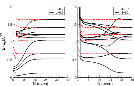
Figure 1: (Color online) Lowest energy levels of the isotropic 2CK model as a function of the number of NRG iterations $N$ ($N$ even) for different initial couplings $J$ and $\Lambda=4$ with 900 states kept at each iteration. As a guide to the eye, the levels obtained in the different NRG iterations $N$ are connected by straight lines. Independently of initial weak-coupling ($J=0.2$), intermediate coupling ($J=0.7$) or strong-coupling ($J=20$) strengths, the same fixed point spectrum is reached. For odd numer of iterations $N$ a non-equidistant fixed point spectrum is obtained as well (not shown).

III NRG treatment and results

For the numerical solution of the 2CK problem we developed an efficient NRG code, following Wilsons’s original algorithm. Wilson (1975) Since for the two-channel model the Hilbert space dimension grows particularly fast with the number $N$ of NRG iterations, i.e. as $16^{N}$, the use of conservation laws is essentual to reduce the Hamiltonian to block structure. The $M$-channel spin-$\frac{1}{2}$ Kondo model has a full symmetry group of $SU(2)_{spin}\times Sp(M)$, where $Sp(M)$ is the symplectic group. Affleck et al. (1992) In the two-channel case ($M=2$), the only decompositions into invariant subgroups of $Sp(2)$ are (i) $SU(2)\times U(1)$, corresponding to channel and charge conservation, and (ii) $SU(2)\times SU(2)$, corresponding to a separate axial charge conservation, used in the work of Pang and Cox. Pang and Cox (1991) In our implementation of the NRG for the 2CK model, we have chosen to use the decomposition (i), where we use the charge $Q$, $z$-component of the total (Kondo) spin $S_{tot}^{z}$ and the $z$-component of the channel spin as labels for the many particle states only, corresponding to the following conserved operators,

$$\hat{Q} = \sum_{n=0,\alpha,\sigma}^{\infty}\left[f_{n\alpha\sigma}^{{\dagger}}f_{n\alpha\sigma}^{\phantom{\dagger}}-\frac{1}{2}\right]$$

$$\hat{S}_{tot}^{z} = \sum_{n=0,\alpha,\sigma}^{\infty}\sigma f_{n\alpha\sigma}^{{\dagger}}f_{n\alpha\sigma}^{\phantom{\dagger}}+S^{z}$$

$$\hat{S}_{ch}^{z} = \frac{1}{2}\sum_{n=0,\alpha,\sigma}^{\infty}\alpha f_{n\alpha\sigma}^{\dagger}f_{n\alpha\sigma}\ .$$

Thus we exploit only the $U(1)$ subgroups of the full $SU(2)$ spin and channel symmetries, respectively. Accordingly, our code effectively uses a $U(1)\times U(1)\times U(1)$ symmetry. This turned out to be an optimal compromize between computatinal efficiency and programming clarity. The Hamiltonians are diagonalized in each irreducible subspace $|Q,S_{tot}^{z},S_{ch}^{z}\rangle$ and about 900 states were sufficient to be retained at each NRG iteration.

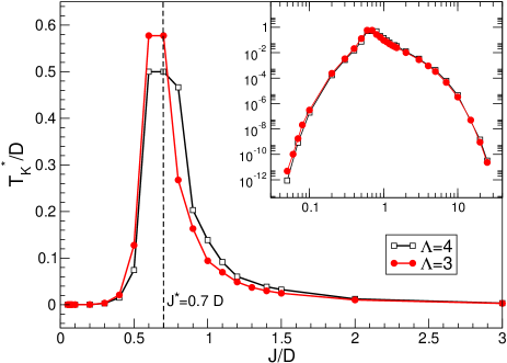
Figure 2: (Color online) Dependence of the Kondo temperature $T_{K}$ on the bare coupling strength $J$ (both in units of $D$), as determined by NRG for $\Lambda=3$ and $\Lambda=4$. The inset shows $T_{K}$ on a logarithmic scale.

After each NRG iteration the Hamiltonian is rescaled by the parameter $\sqrt{\Lambda}$, $\Lambda>1$. Wilson (1975) The correct convergence of the NRG procedure was checked by comparing the results obtained with two different $\Lambda$-values, $\Lambda=3$ and $\Lambda=4$. It yielded excellent quantitative agreement, as seen below in Fig. 3.

We have solved the isotropic 2CK model for a wide range of bare spin couplings $J$ in order to determine the $J$-dependence of $T_{K}$. Typical flow diagrams of the energy eigenvalues are shown in Fig. 1, exhibiting non-equidistant level spacings characteristic for the non-Fermi liquid fixed point. Cox and Zawadowski (1998) The fixed point coupling $J^{*}$ is characterized by the fact that, when the inital coupling is $J=J^{*}$, the energy eigenvalues settle immediately (after 1 or 2 iterations) to their fixed point values (red dashed curves in Fig. 1). It is thus identified as $J^{*}\approx 0.7D$ in agreement with Ref. Pang and Cox, 1991. Following standard procedures, the Kondo temperature $T_{K}$ can be determined as the energy scale either where the energy flow diagrams have an inflection point or where the first excited energy level has reached its fixed point value within, e.g., 10 percent. Both definitions of this crossover scale are equivalent up to a constant prefactor, as seen for the weak coupling region in Fig. 3. Since, however, in the strong coupling region, $J>J^{*}$, the complexity of the level flow makes it difficult to identify a single inflection point (see Fig.1), we adopt the second definition.

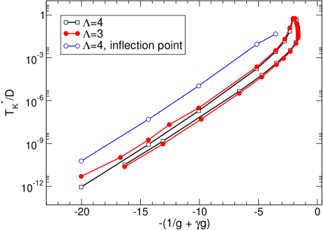
Figure 3: (Color online) The Kondo temperature $T_{K}$ is shown on a logarithmic scale versus the parameter $-(\frac{1}{\rho_{0}J}+\gamma\rho_{0}J)$, $\gamma=30/46\approx 2/3$. The upper branch of the curves corresponds to the weak coupling, the lower branch to the strong coupling regime. The results for $T_{K}$ obtained from the “inflection point method” (see text) in the weak coupling regime ($J<J^{*}$) are shown for comparison and differ only by a constant prefactor.

Our results for the dependence of $T_{K}$ on the bare Kondo coupling $J$ are shown in Fig. 2. It shows a strong peak at around $J=0.7D$, as expected. The results for the two discretizations considered, $\Lambda=3$, $\Lambda=4$, show no significant differences. The deviations in the intermediate coupling regime around the peak maximum in Fig. 2 arise from the difficulty to determine the exact $T_{K}^{*}$ when the crossover happens at the very beginning of the NRG iterations where the energy resolution is low. The behavior of $T_{K}^{*}$ is examined over nearly three decades of $J$ and extends over more than 10 decades in $T_{K}^{*}$, as illustrated in the inset of Fig. 2.

The $J$-dependence of $T_{K}$ can be further analysed by plotting it in Fig. 3 versus the parameter $-(1/g+\gamma g)$. It shows the exponential behavior of $T_{K}$ as a function of $1/J$ in the weak coupling limit $1/J\rightarrow\infty$ and as a function of $J$ in the strong coupling limit $1/J\rightarrow\infty$, with logarithmic corrections towards the intermediate coupling regime, in agreement with Eqs. 2 and 11. Note that the strong coupling and the weak coupling branches in Fig. 3 are parallel to each other, i.e. the NRG quantitaively confirms the analytical value of the parameter $\gamma=30/46$. The shift of the two branches can be traced back to the fact the strong coupling Anderson impurity model, Eq. (24), produces higher-order logarithmic corrections which are different from those of the weak coupling model, Eq. (1) and which are, thus, not included in the effective low-energy 2CK model, Eq. (10).

IV Conclusion

The two-channel Kondo model exhibits for low energies a duality between the regions of weak and strong bare Kondo coupling $J$. This results from the fact that in both limits, $J\to 0$ and $J\to\infty$ the ground state is doubly degenerate. While for $J\to 0$ it is the decoupled impurity spin doublet, for $J\to\infty$ it is a doubly degenerate quantum frustrated 3-body state, comprised of the impurity spin and the conduction electron spins located at the impurity site in each of the two channels. We have shown that, hence, the complete strong coupling behavior can be obtained from the solution in the weak coupling regime via the identification of the dimensionless coupling, $\gamma g\to 1/g$, where $\gamma=30/46\approx 2/3$. These results have been confirmed quantitatively by the exact numerical renormalization group solution of the problem.

As a result, the dependence of the Kondo temperature $T_{K}$ on the $J$ is strongly peaked at the two-channel Kondo fixed point coupling, $J=J^{*}\approx 0.7$, and decays exponentially both for small and for large couplings. The maximum is of the order of the band cutoff, $T_{K}(J^{*})\approx D$, with non-Fermi liquid behavior for all energies below $T_{K}$.

We conjecture that this could be the reason why in experimental conductance anomalies of nanoconstrictions with two-channel Kondo signatures Ralph and Buhrman (1992, 1995); v. Delft et al. (1998) no broad distribution of $T_{K}$ is observed: The band cutoff and hence $T_{K}(J^{*})$ in two-channel Kondo systems can be provided by a decoherence scale of the order of a few Kelvin. Aleiner et al. (2001) This would mean that, even if there is a broad distribution of bare couplings, only for those couplings sufficiently close to $J^{*}$ the non-Fermi liquid behavior would extend up to sufficiently high energies to be observable. However, more detailed calculations as well as a detailed microscopic model for the two-channel Kondo defects will be required to substantiate this conjecture.

Appendix A Details on the duality analysis

Destruction of an electron from the 3-particle compound ground states (Eqs. 4), (5) in channel $\alpha=\pm 1$ generates the (unnormalized) states,

$$\begin{array}[]{rclcl}c_{0\uparrow 1}|\Psi_{\uparrow}^{0}\rangle&=&\frac{2}{\sqrt{6}}|0\Downarrow\uparrow\rangle-\frac{1}{\sqrt{6}}|0\Uparrow\downarrow\rangle&=&\frac{\sqrt{3}}{2}|\Psi_{00-1}\rangle+\frac{1}{\sqrt{12}}|\Psi_{10-1}\rangle\\ c_{0\downarrow 1}|\Psi_{\uparrow}^{0}\rangle&=&-\frac{1}{\sqrt{6}}|0\Uparrow\uparrow\rangle&=&-\frac{1}{\sqrt{6}}|\Psi_{11-1}\rangle\\ c_{0\uparrow-1}|\Psi_{\uparrow}^{0}\rangle&=&\frac{2}{\sqrt{6}}|\uparrow\Downarrow 0\rangle-\frac{1}{\sqrt{6}}|\downarrow\Uparrow 0\rangle&=&\frac{\sqrt{3}}{2}|\Psi_{001}\rangle+\frac{1}{\sqrt{12}}|\Psi_{101}\rangle\\ c_{0\downarrow-1}|\Psi_{\uparrow}^{0}\rangle&=&-\frac{1}{\sqrt{6}}|\Uparrow\uparrow 0\rangle&=&-\frac{1}{\sqrt{6}}|\Psi_{111}\rangle\\ c_{0\uparrow 1}|\Psi_{\downarrow}^{0}\rangle&=&-\frac{1}{\sqrt{6}}|0\Downarrow\downarrow\rangle&=&-\frac{1}{\sqrt{6}}|\Psi_{1-1-1}\rangle\\ c_{0\downarrow 1}|\Psi_{\downarrow}^{0}\rangle&=&\frac{2}{\sqrt{6}}|0\Uparrow\downarrow\rangle-\frac{1}{\sqrt{6}}|0\Downarrow\uparrow\rangle&=&-\frac{\sqrt{3}}{2}|\Psi_{00-1}\rangle+\frac{1}{\sqrt{12}}|\Psi_{10-1}\rangle\\ c_{0\uparrow-1}|\Psi_{\downarrow}^{0}\rangle&=&-\frac{1}{\sqrt{6}}|\downarrow\Downarrow 0\rangle&=&-\frac{1}{\sqrt{6}}|\Psi_{1-11}\rangle\\ c_{0\downarrow-1}|\Psi_{\downarrow}^{0}\rangle&=&\frac{2}{\sqrt{6}}|\downarrow\Uparrow 0\rangle-\frac{1}{\sqrt{6}}|\uparrow\Downarrow 0\rangle&=&-\frac{\sqrt{3}}{2}|\Psi_{001}\rangle+\frac{1}{\sqrt{12}}|\Psi_{101}\rangle\end{array}$$ (21)

which can be expressed in terms of the strong coupling singlet/triplet eigenstates Eqs. (6)-(9) as indicated. We define bosonic creation operators for the latter states,

$$|\Psi_{sm\alpha}\rangle=B^{\dagger}_{sm\bar{\alpha}}|vac\rangle\ ,$$ (22)

which transform with respect to the channel SU(2) group according to the adjoint representation, i.e. $\bar{\alpha}=-\alpha$. Together with the fermionic operators of Eqs. (4), (5) they satisfy the constraint

$$\hat{Q}=\sum_{\sigma}F^{\dagger}_{\sigma}F^{\phantom{\dagger}}_{\sigma}+\sum_{sm\bar{\alpha}}B^{\dagger}_{sm\bar{\alpha}}B^{\phantom{\dagger}}_{sm\bar{\alpha}}=1\ ,$$ (23)

an expression of the uniqueness of the strong coupling basis states. In the strong coupling basis, using Eq. (21) the 2CK Hamiltonian (1) then takes form of a generalized two-channel Anderson impurity model in one dimension,

$$H= t\sum_{\langle i,j\rangle\ i,j\neq 0}\sum_{\alpha\sigma}c_{i\alpha\sigma}^{\dagger}c_{j\alpha\sigma}^{\phantom{\dagger}}-J\sum_{\sigma}F_{\sigma}^{\dagger}F_{\sigma}^{\phantom{\dagger}}-\frac{3}{4}J\sum_{\alpha}B_{00\bar{\alpha}}^{\dagger}B_{00\bar{\alpha}}^{\phantom{\dagger}}+\frac{1}{4}J\sum_{m=0,\pm 1\alpha}B_{1m\bar{\alpha}}^{\dagger}B_{1m\bar{\alpha}}^{\phantom{\dagger}}$$ (24)

$$+\ t\sum_{i=\pm 1}\sum_{\alpha}\left[\frac{\sqrt{3}}{2}c_{i\alpha\uparrow}^{\dagger}B_{00\bar{\alpha}}^{\dagger}F_{\uparrow}^{\phantom{\dagger}}-\frac{1}{\sqrt{6}}c_{i\alpha\downarrow}^{\dagger}B_{1+1\bar{\alpha}}^{\dagger}F_{\uparrow}^{\phantom{\dagger}}+\frac{1}{\sqrt{12}}c_{i\alpha\uparrow}^{\dagger}B_{10\bar{\alpha}}^{\dagger}F_{\uparrow}^{\phantom{\dagger}}\right.$$

$$\hskip 49.79231pt\left.-\frac{\sqrt{3}}{2}c_{i\alpha\downarrow}^{\dagger}B_{00\bar{\alpha}}^{\dagger}F_{\downarrow}^{\phantom{\dagger}}-\frac{1}{\sqrt{6}}c_{i\alpha\uparrow}^{\dagger}B_{1-1\bar{\alpha}}^{\dagger}F_{\downarrow}^{\phantom{\dagger}}+\frac{1}{\sqrt{12}}c_{i\alpha\downarrow}^{\dagger}B_{10\bar{\alpha}}^{\dagger}F_{\downarrow}^{\phantom{\dagger}}+H.c.\right]\ ,$$

where $V=2t$ plays the role of the band-impurity hybridization and the factor 2 arises from the fact that there is hopping from the impurity site $0$ to the two sites $i=\pm 1$. By means of a Schrieffer-Wolff transformation Schrieffer and Wolff (1966) this Hamiltonian maps for energies $\omega\ll J$ onto the effective 2CK model Eq. (10), where potential scattering terms have been neglected. Since only the intermediate (bosonic) states with $m=0$ contribute to an effective Kondo spin flip (i.e. only products of the 1st and the 4th term and of the 3rd and the 6th term of the hybridization part in Eq. (24)), the effective spin flip coupling, as defined through Eq. (10) reads,

$$\tilde{J}=2\frac{4t^{2}}{J}\left(\frac{\frac{3}{4}}{1-\frac{3}{4}}+\frac{\frac{1}{12}}{1+\frac{1}{4}}\right)=\frac{1}{\gamma}\frac{(4t)^{2}}{J}\ ,$$

where $\gamma=30/46\approx 2/3$.

References

- Kondo (1964) J. Kondo, Prog. Theor. Phys. 32, 37 (1964).
- Nozières and Blandin (1980) P. Nozières and A. Blandin, Journal de Physique (Paris) 41, 193 (1980).
- Hewson (1993) A. C. Hewson, The Kondo Problem to Heavy Fermions (Cambridge University Press, 1993).
- Andrei and Destri (1984) N. Andrei and C. Destri, Phys. Rev. Lett. 52, 364 (1984).
- Tsvelick and Wiegmann (1984) A. M. Tsvelick and P. B. Wiegmann, Z. Phys. B 54, 201 (1984).
- Coleman et al. (1995) P. Coleman, L. B. Ioffe, and A. M. Tsvelik, Phys. Rev. B 52, 6611 (1995).
- Affleck and Ludwig (1991) I. Affleck and A. W. W. Ludwig, Nucl. Phys. B 352, 849 (1991).
- Ludwig and Affleck (1991) A. W. W. Ludwig and I. Affleck, Phys. Rev. Lett. 67, 3160 (1991).
- Affleck and Ludwig (1993) I. Affleck and A. W. W. Ludwig, Phys. Rev. B 48, 7297 (1993).
- Black et al. (1982) J. L. Black, K. Vladár, and A. Zawadowski, Phys. Rev. B 26, 1559 (1982).
- Cox and Zawadowski (1998) D. L. Cox and A. Zawadowski, Adv. Phys. 47, 599 (1998).
- Aleiner et al. (2001) I. L. Aleiner, B. L. Altshuler, Y. M. Galperin, and T. A. Shutenko, Phys. Rev. Lett. 86, 2629 (2001).
- Zaránd (2005) G. Zaránd, Phys. Rev. B 72, 245103 (2005).
- Seaman et al. (1991) C. L. Seaman et al., Phys. Rev. Lett. 67, 2882 (1991).
- Cox (1987) D. L. Cox, Phys. Rev. Lett. 59, 1240 (1987).
- Cichorek2CK (2005) T. Cichorek et al., Phys. Rev. Lett. 94, 236603 (2005).
- Ralph and Buhrman (1992) D. C. Ralph and R. A. Buhrman, Phys. Rev. Lett. 69, 2118 (1992).
- Ralph and Buhrman (1995) D. C. Ralph and R. A. Buhrman, Phys. Rev. B 51, 3554 (1995).
- Keijsers et al. (1996) R. J. P. Keijsers, O. I. Shklyarevskii, and H. van Kempen, Phys. Rev. Lett. 77, 3411 (1996).
- Gupta et al. (2005) J. A. Gupta, C. P. Lutz, A. J. Heinrich, and D. M. Eigler, Phys. Rev. B 71, 115416 (2005).
- v. Delft et al. (1998) J. v. Delft et al., Ann. Phys. 263, 1 (1998).
- Ralph et al. (1994) D. C. Ralph, A. W. W. Ludwig, J. v. Delft, and R. A. Buhrman, Phys. Rev. Lett. 72, 1064 (1994).
- Hettler et al. (1994) M. H. Hettler, J. Kroha, and S. Hershfield, Phys. Rev. Lett. 73, 1967 (1994).
- Wingreen et al. (1995) N. S. Wingreen, B. L. Altshuler, and Y. Meir, Phys. Rev. Lett. 75, 769 (1995).
- Ralph et al. (1995) D. C. Ralph, A. W. W. Ludwig, J. v. Delft, and R. A. Buhrman, Phys. Rev. Lett. 75, 770 (1995).
- Kozub and Rudin (1997) V. I. Kozub and A. M. Rudin, Phys. Rev. B 55, 259 (1997).
- Goldhaber-Gordon et al. (1006) R. M. Potok, I. G. Rau, H. Shtrikman, Y. Oreg, and D. Goldhaber-Gordon, cond-mat/0610721.
- Oreg and Goldhaber-Gordon (2003) Y. Oreg and D. Goldhaber-Gordon, Phys. Rev. Lett. 90, 136602 (2003).
- Yanson et al. (1995) I. K. Yanson et al., Phys. Rev. Lett 74, 302 (1995).
- Zaránd and Udvardi (1996) G. Zaránd and L. Udvardi, Phys. Rev. B 54, 7606 (1996).
- Florens (2004) S. Florens, Phys. Rev. B 69, 113103 (2004).
- Schrieffer and Wolff (1966) J. R. Schrieffer and P. A. Wolff, Phys. Rev. 149, 491 (1966).
- Wilson (1975) K. G. Wilson, Rev. Mod. Phys. 47, 773 (1975).
- Affleck et al. (1992) I. Affleck, A. W. W. Ludwig, H. B. Pang, and D. L. Cox, Phys. Rev. B 45, 7918 (1992).
- Pang and Cox (1991) H. B. Pang and D. L. Cox, Phys. Rev. B 44, 9454 (1991).