Global Partial Density of States: Statistics and Localization Length in Quasi-one Dimensional disordered systems

Abstract

We study the distributions functions for global partial density of states (GPDOS) in quasi-one-dimensional (Q1D) disordered wires as a function of disorder parameter from metal to insulator. We consider two different models for disordered Q1D wire: a set of two dimensional $\delta$ potentials with an arbitrary signs and strengths placed randomly, and a tight-binding Hamiltonian with several modes and on-site disorder. The Green functions (GF) for two models were calculated analytically and it was shown that the poles of GF can be presented as determinant of the rank $N\times N$, where $N$ is the number of scatters. We show that the variances of partial GPDOS in the metal to insulator crossover regime are crossing. The critical value of disorder $w_{c}$ where we have crossover can be used for calculation a localization length in Q1D systems.

I Introduction

Calculation of density of states (DOS) allowed us obtain many properties of the system under consideration, such as charging effects, electrical conduction phenomena, tunneling spectroscopy or thermodynamic properties. Furthermore, the decomposition of DOS in partial density of states (PDOS) and global PDOS (GPDOS), which appear naturally in scattering problems in which one is concerned with the response of the system to small perturbation $\delta U(x)$ of the potential $U(x)$, plays an important role in dynamic and nonlinear transport in mesoscopic conductors Buttiker93 ; Buttikeral94 ; Brand98 ; Zhengal97 ; Gasparian96 ; Buttiker01 ; Schomerusal02 ; Buttiker02 . Particularly the emissivity, which is the PDOS in configuration space for electrons emitted through arbitrary lead Buttikeral94 ; B98 ; SM99 , always present in physical phenomena where quantum interference is important. As shown in MB02 the heat flow, the noise properties of an adiabatic quantum pump can expressed in terms of generalized parametric emissivity matrix $\nu[X]$ (the diagonal element $\nu_{\alpha\alpha}[X]$ of which is the number of electrons entering or leaving the device in response to small change $\delta U(x)$, such as a distortion of the confining potential). The nondiagonal element $\nu_{\alpha\beta}[X]$ of parametric emissivity matrix determines the correlation between current in the contacts $\alpha$ and $\beta$ due to a variation of parameter $X$ MB02 . Note that the elements of GPDOS are closely related to characteristic times of the scattering process, consequently, to the absolute square of the scattering states. Particularly in 1D systems $\nu_{\alpha\beta}$ and $\nu_{\alpha\alpha}$ are related to Larmor transmitted time $\tau_{T}$ (or Wigner delay time) and reflected time $\tau_{R}$ weighted by the transmission coefficient $T$ Gasparian96 ; Prigodin99 and reflection coefficient $R$, respectively. As it was mentioned by Büttiker and Christen BC98 the dynamic response of the system to an external time dependent perturbation, i.e., the emittance in general not capacitance-like, i.e. the diagonal and the off-diagonal emittance elements are not positive and negative values, respectively. Whenever the transmission of carriers between two contacts predominates the reflection, the associated emittance element changes sing and behaves inductance-like. This type of cross over behavior for diagonal element of emittance $\nu_{\alpha\alpha}$ (taking into account the Coulomb interaction of electrons inside the sample) was found in Tiago00 where they study the distribution function (DF) of emittance. They have found that in the range of weak disorder, when the system is still conducive the DF is Gaussian-like. With increasing disorder the DF becomes non-Gaussian.

The purpose of this paper is to study numerically the behaviors of DF of diagonal $\nu_{\alpha\alpha}$ and off-diagonal elements $\nu_{\alpha\beta}$ of global PDOS in the Q1D disordered wires, where not so much known about the DF. We study three different regimes of transport: metallic ($\xi>>L$), where $\xi$ is the localization length and $L$ the typical size of the system, insulating ($\xi<<L$) and crossover ($\xi\sim L$). We show that in intermediate regime of transport between the metallic and insulating regimes there is the critical value of disorder $w_{c}$ when we observe cross over between the variances var($\nu_{\alpha\alpha}$) and var($\nu_{\alpha\beta}$) (see Fig.1). This critical $w_{c}$ determines the localization length of Q1D system for given length $L$ and number of modes $M$. It turns out that in metallic regime $P(\nu_{\alpha\beta})$ is Gaussian which means that the first and the second moments (i.e., the average $<\nu_{\alpha\beta}>$ and the variance var($\nu_{\alpha\beta})=<\nu_{\alpha\beta}^{2}>-{<\nu_{\alpha\beta}>}^{2}$) are enough to describe the behavior of $P(\nu_{\alpha\beta})$. In the strong localization regime the distribution of $\nu_{\alpha\beta}$ is log normal, which means that the $\ln\nu_{\alpha\beta}$ follows a Gaussian distribution. As regards the distribution function of $\nu_{\alpha\alpha}$ we can say that in the strong localization regime it characterized by an exponential tail, the values of $\nu_{\alpha\alpha}$ are positive and that the dynamic response of the system is capacitivelikeBC98 . In the metallic regime the emittance has non Gaussian-like behavior and some of the value of $\nu_{\alpha\alpha}$ are negative (inductivelike behavior)Tiago00 .

The paper is organized as follows. In the next section we present our model and set the basis on numerical calculation for obtaining the probability distributions of $\nu_{\alpha\alpha}$ and $\nu_{\alpha\beta}$ for different regimes. In section III we study the behavior of var($\nu_{\alpha\alpha}$) and var($\nu_{\alpha\beta}$) as a function of disorder strength $w$. In section IV we calculate the distribution functions for $\nu_{\alpha\alpha}$ and $\nu_{\alpha\beta}$ in three different regimes of transport mentioned in Introduction. The paper is included in section V.

II The model and numerical procedures

The localization length $\xi$ is obtained from the decay of the average of the logarithm of the conductance, $\ln g$, as a function of the system size $L$

$$\xi^{-1}=-\lim_{L\rightarrow\infty}\frac{1}{2L}<\ln g>$$ (1)

where $g$ is given by Büttiker-Landauer formula Landauer89 ; Datta95 ($T_{nm}$ is the transmission coefficient from mode $n$ to mode $m$)

$$g=\frac{2e^{2}}{h}\sum_{n,m}T_{nm},$$ (2)

We will consider two models: Q1D wire with the set of $\delta$ scattering potentials of the form

$$V(x,y)=\sum_{n=1}^{N}V_{n}\delta(x-x_{n})\delta(y-y_{n}),$$ (3)

with $V_{n}$, $x_{n}$ and $y_{n}$ be arbitrary parameters and Q1D lattice of size $L\times W$ ($L\gg W$, $L$ is the length and $W$ is the width of the system), where the site energy can be chosen randomly. In both cases analytically we have calculated the Green’s function of 1QD (RG06 ) and use them in our numerical calculations (see Appendix). The elements of global PDOS $\nu_{\alpha\beta}$, in the case of a tight-binding model can be calculate in terms of the scattering matrix and the Green Function. To calculate the scattering matrix elements, corresponding to transmission between modes n and m, we start from the Fisher-Lee relation Fisherlee81 ; Datta95 , which expresses these elements in terms of the Green’s function:

$$s_{nm}={-\delta_{nm}+\imath\hbar\sqrt{v_{n}v_{m}}\sum_{i,j}\chi_{n}\left(r_{0_{i}}\right)G\left(r_{0_{i}},r_{0_{j}}\right)\chi_{m}\left(r_{0_{j}}\right)}.$$ (4)

$\chi_{m}\left(r_{0_{j}}\right)$ is the transverse wavefunction corresponding to mode m at the point $r_{0_{j}}$ and $G\left(r_{0_{i}},r_{0_{j}}\right)$ is the Green’s function (GF) for non coinciding coordinates. $v_{m}$ is the velocity associated with propagating mode $m$. The LPODS is directly connected to the S-matrix elements $s_{nm}$ through the expression Buttiker93 :

$$\frac{dn_{nm}(r)}{dE}\equiv-\frac{1}{4\pi\imath}\left(s_{nm}^{*}\frac{\delta s_{nm}}{\delta U(r)}-\frac{\delta s_{nm}^{*}}{\delta U(r)}s_{nm}\right)$$ (5)

Insertion of Eq. (4) in Eq. (5) gives:

$$\frac{dn_{nm}}{dE}(r)=-\frac{\hbar\sqrt{v_{n}v_{m}}}{4\pi}\sum_{i,j}\left(s_{mn}^{*}\chi_{n}(r_{0_{i}})G(r_{0_{i}},r)G(r,r_{0_{j}})\chi_{m}(r_{0_{j}})\break+H.c.\right)$$ (6)

where H.c. denotes Hermitian conjugate. To arrive the above expression we have calculated the functional derivative of the Green’s function by adding to the Hamiltonian of our system the local potential variation $\delta U(r)=\delta U_{a}\delta(r-r_{a})$ ($\delta U_{a}\rightarrow 0$), which lead us to the relation Gasparian96

$$\frac{\delta G(r_{n},r_{m})}{\delta U(r)}=G(r_{n},r)G(r,r_{m}).$$

Once we have calculated the local PDOS we can obtain the global PDOS adding the local PDOS over the particles of our system:

$$\frac{dN_{nm}}{dE}=\sum_{k}\frac{dn_{nm}(r_{k})}{dE}$$ (7)

After summation over the indices $i,j$ and $r_{k}$ the above equation in matrix form can be presented:

$$\frac{dN_{nm}}{dE}=-\frac{\hbar\sqrt{v_{n}v_{m}}}{4\pi}(s_{mn}^{*}Q_{nm}+H.c)$$ (8)

where $Q_{nm}$ matrix defined as

$$Q_{mn}=\tilde{\chi}_{n}\left(\sum_{j=1}^{M}G_{mj}G_{jn}\right)\tilde{\chi}_{m}^{T}$$ (9)

$\tilde{\chi_{n}}$ is the column matrix:

$$\tilde{\chi}=\left(\begin{array}[]{c}\chi_{n}(1)\\ \vdots\\ \chi_{n}(M)\end{array}\right)$$ (10)

Here $\tilde{\chi}_{m}^{T}$ is the transpose of the column matrix $\tilde{\chi}_{m}$ and $G_{mj}$ is the matrix of $M\times M$ rank ($M$ is the number of modes in each lead, see Appendix).

Finally, $\nu_{\alpha\alpha}$ and $\nu_{\alpha\beta}$ one can get from global PDOS ${dN_{nm}}/{dE}$ by summing every mode $n$ in lead $\alpha$ and every mode $m$ in lead $\beta$ respectively:

$$\nu_{\alpha\alpha}=\sum_{n,m\in\alpha}\frac{dN_{nm}}{dE}$$ (11)

$$\nu_{\alpha\beta}=\sum_{n\in\alpha,m\in\beta}\frac{dN_{nm}}{dE}$$ (12)

Similarly can be written also $\nu_{\beta\beta}$ and $\nu_{\beta\alpha}$ and so global DOS $\nu$ must be sum of all GPDOS:

$$\nu=\nu_{\beta\beta}+\nu_{\alpha\alpha}+\nu_{\alpha\beta}+\nu_{\beta\alpha}.$$ (13)

In the case of the Q1D wire with the set of $\delta$ potentials (see Eq. (3)) in quantities (7), (11) and (12)), calculated for tight-binding model one must replace the sign of summation by appropriate spatial integration.

For numerical study we consider a quasi-one dimensional lattice of size $L\times W$ ($L\gg W$), where $L$ is the length and $W$ is the width of the system. The standard tight-binding Hamiltonian with nearest-neighbor interaction

$$H=\sum_{i}\epsilon_{i}\mid r_{i}><r_{i}\mid-t\sum_{i,j}\mid r_{i}><r_{j}\mid,$$ (14)

where $\epsilon_{i}$ is the energy of the site $i$ chosen randomly between $\left(-\frac{w}{2},\frac{w}{2}\right)$ with uniform probability. The double sum runs over nearest neighbors. The hopping matrix element $t$ is taken equal to $1$, which sets the energy scale, and the lattice constant equal to $1$, setting the length scale. The energies are measured with respect to the center of the band so we will always deal with propagating modes. Finally our sample is connected to two semi-infinite, multi-modes leads to the left (lead $\alpha$) and to the right (lead $\beta$). For simplicity we take the numbers of modes in the left and right leads to be the same ($M$) and so the width of this system $w$ becomes equal $M$ (for a tight-binding model the numbers of modes coincides with the number of sites in the transverse direction). The conductance of a finite size sample depends on the properties of the system and also on the leads which must be taken into account in a appropriate way. In order to take into account the interaction of the conductor with the leads we introduce a self-energy term ”$A$” as an effective Hamiltonian, which will be calculated as (see, e.g. Datta95 )

$$A_{p}(r_{0_{i}},r_{0_{j}})=-t\sum_{m\epsilon p}\chi_{m}(r_{0_{i}})e^{\imath k_{m}a}\chi_{m}(r_{0_{j}})$$ (15)

$$A_{q}(r_{0_{l}},r_{0_{k}})=-t\sum_{n\epsilon q}\chi_{n}(r_{0_{l}})e^{\imath k_{n}a}\chi_{n}(r_{0_{k}})$$ (16)

$$A=A_{p}+A_{q}$$ (17)

Finally for numerical calculation of DF of var($\nu_{\alpha\alpha}$) and var($\nu_{\alpha\beta}$) for $M\gg 1$ and for higher dimension of the system we calculate the Green function as:

$$G=[E\hat{I}-\hat{H}-\hat{A}]^{-1}$$ (18)

To perform numerical calculation of the elements of this Green’s matrix we will use Dyson’s equation, as in Mackinnon85 ; Verges99 , propagating strip by strip. This drastically reduced the computational time, because instead to inverting an $L^{2}\times M^{2}$ matrix, we just have to invert $L$ times $L\times M$ matrices. In this way we build the complete lattice starting from a single strip, and introducing one by one the interaction with the next strip. Each time we introduce a new strip we apply the recursion relations of Dyson’s equation, until we finally obtain the Green function for the complete lattice. Once we have the Green’s function matrix we calculate var($\nu_{\alpha\alpha}$) and var($\nu_{\alpha\beta}$) according to Eqs. (11) and (12), and obtain their probability distributions for random potentials. Over 250000 independent impurity configurations where averaged for each $N$.

III var($\nu_{\alpha\alpha})$ and var($\nu_{\alpha\beta}$) vs $w$

In this section we are going to study the dependance of the var($\nu_{\alpha\alpha})$ and var($\nu_{\alpha\beta}$) vs disorder $w$ and vs the number of mode $M$. In Fig.1 we show the behavior of var($\nu_{\alpha\alpha})$ and var($\nu_{\alpha\beta}$) as a function of the disorder $w$. Plot is for a sample of $L=400$ and $M=4$. The crossover define a critical value of the disorder $w_{c}$. In Fig.2 we show the dependence of the critical value $w_{c}$ with the number of modes $M$ for several samples. As one can see with increasing the number of modes the crossing point moves to the left and the $w_{c}$ decreases. This means that in the weak localized regime, in analogy with 1D systems the ratio of localization length $\xi$ to the longitudinal size of the sample $L$ for given modes $M$ follows, in a good approximation, a law of the form

$$\frac{\xi}{L}\simeq C(M,w_{c},E)$$ (19)

where $C$ is a constant that depends from the $M$, $w_{c}$ and energy. With appropriate choice of an effective length $L_{eff}=L(a+bM^{c})$ (with $a=0.967$, $b=0.035$ and $c=2.33$) we were able to show that all the curves presented in the Fig.2 collapse into universal curve in Q1D system, supporting the applicability of the hypothesis of single-parameter scalingAALR79 in disordered systems. In Fig.3 we plot this curve for $w_{c}$ as a function of $1/L_{eff}$. The different values of modes are specified inside the figure.

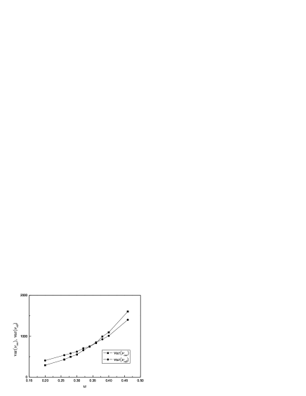
Figure 1: Crossover between var($\nu_{\alpha\alpha})$ and var($\nu_{\alpha\beta}$) for sample of $L=400$ and $M=4$.

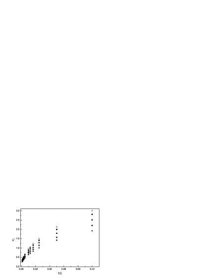
Figure 2: Critical value $w_{c}$ for several samples as a function of $1/L$: $\circ$ is for 1D sample; $\bullet$, $\blacktriangle$, $\blacktriangledown$ and $\star$ are for quasi 1D samples with the numbers of mode $M=2,3,4,5$, respectively.

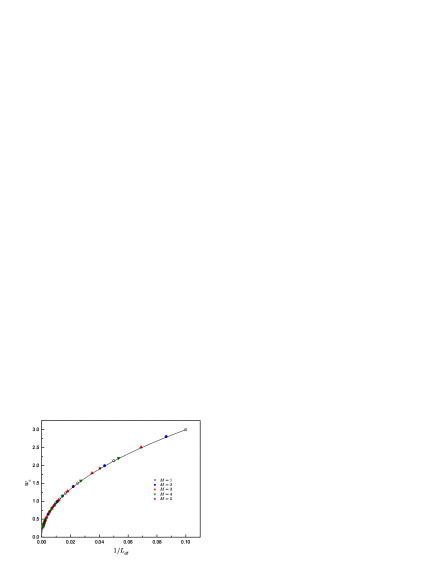
Figure 3: Universal curve $w_{c}$ for several samples as a function of $1/L_{eff}$. $\circ$ is for 1D sample; $\bullet$, $\blacktriangle$, $\blacktriangledown$ and $\star$ are for quasi 1D samples with the numbers of mode $M=2,3,4,5$, respectively.

In strictly 1D system, following Gasparian96 one can write ($\nu_{T}\equiv\nu_{\alpha\beta}+\nu_{\beta\alpha}$ and $\nu_{R}\equiv\nu_{\alpha\alpha}+\nu_{\beta\beta}$)

$$\left\langle\ln\nu_{R}\right\rangle=\left\langle\ln\nu\right\rangle+\left\langle\ln R\right\rangle$$ (20)

$$\left\langle\ln\nu_{T}\right\rangle=\left\langle\ln\nu\right\rangle+\left\langle\ln T\right\rangle$$ (21)

where $R$ and $T$ are the reflection and transmission coefficients respectively and $\left\langle...\right\rangle$ denotes averaging over ensemble. Using the asymptotic behavior of $<\ln T>$ and $<\ln R>$ as $L\to\infty$ (see, e.g. Gredeskul ) these expressions in weak disorder regime can be rewritten as:

$$\left\langle\ln\nu_{R}\right\rangle=\left\langle\ln\nu\right\rangle+\ln(1-e^{-2L/\xi})$$ (22)

$$\left\langle\ln\nu_{T}\right\rangle=\left\langle\ln\nu\right\rangle-2L/\xi$$ (23)

In Fig.4 we plot average of $\ln\nu_{R}$ and $\ln\nu_{T}$ for different values of disorder $w_{c}$ as a function $L/\xi$. We see that numerical data for these quantities very well coincide with Eqs. (22) and (23) for small $w_{c}$ or for large $L/\xi$.

Figure 4: Average of $\ln\nu_{R}$ and $\ln\nu_{T}$ as a function $L/\xi$. Solid curves are given by Eqs. (22) and (23). The data points ($\bullet$) are the numerical results for a sample of $L=400$.

IV Plots and Discussions

We are analyzed the DF $P(\nu_{\alpha\alpha})$ and $P(\nu_{\alpha\beta})$ along the transition from the metallic to the insulating regime for several samples sizes. We found that the relative shape of the DF depends only from the disorder parameter $L/\xi$, i.e. with increasing of the number of modes $M$ we always can find an appropriate range of $w$ for which all the curves have the same form. Therefore in the rest of the section, without losing generality we present our results for a sample of $L=400$ and $M=4$ for several values of the disorder $w$.

In the metallic regime when the system size much smaller than the localization length $L<<\xi$ the distribution functions are shown in Fig.5 with ($W=0.2$, $L/\xi=0.17$ and $\langle g\rangle=2.52$). We have checked that the distribution of $P(\nu_{\alpha\beta})$ is Gaussian-like and can be fit with the following expression ($B=1.0$, $\mu=116.5$ and $\sigma=20.2$):

$$P(\nu_{\alpha\beta})=\frac{B}{\sqrt{2\pi}\sigma}e^{-{(\nu_{\alpha\beta}-\mu)^{2}}/{2\sigma^{2}}}.$$ (24)

In spite of the fact that in our numerical studies we deal with Q1D systems where the numbers of modes $M>1$, still the Gaussian-like behavior of the $\nu_{\alpha\beta}$ in ballistic regime can be understood well if we recall the fact that $\nu_{\alpha\beta}$ connected with physically meaning full times characterizing the tunneling process Gasparian96 . In 1D systems GPDOS is related to Larmor transmitted time $\tau_{T}$ (or Wigner delay time) weighted by the transmission coefficient Gasparian96 ; Prigodin99 ,

$$\nu_{\alpha\beta}={\frac{T}{2}}\tau_{T},$$ (25)

The quantity $\tau_{T}$, which links to the density of states of the system GP93 and can be presented

$$\tau_{T}=\hbar{Im}\int_{0}^{L}G(x,x)\,dx=\hbar{Im}\left\{{\frac{\partial\ln t}{\partial E}}+{\frac{r+r^{\prime}}{4E}}\right\}$$ (26)

where $G(x,x)$ is the GF for the whole system, $t$ and $r$ are the transmission and reflection amplitudes from the finite system. $r^{\prime}$ is the reflection amplitude of the electron from the whole system, when it falls in from the right.

The second term in Eq. (26) becomes important for low energies and/or short systems. This term can be neglected in the semiclassical WKB case and, of course, when $r$ (and so $r^{\prime}$) is negligible, e.g., in the resonant case, when the influence of the boundaries is negligible. Of course the distribution function of $\nu_{\alpha\beta}$ (Eq. (25)) is affected by correlations between the value of the DOS (or Wigner delay time) and the transmission coefficient of resonances via localized states, but still it can capture some general behavior Wigner delay time in 1D system in the regime where $T\sim 1$. Wigner delay time in 1D and in the ballistic regime is given by Gaussian function and can be characterized by a first moment and a second cumulant Texiercomtet99 ; Heinrichs02 .

Similar relation to Eq. (25) holds for $\nu_{\alpha\alpha}$:

$$\nu_{\alpha\alpha}={\frac{R}{2}}\tau_{R},$$ (27)

where $\tau_{R}$ characterize the reflection time and defined as:

$$\tau_{R} = \hbar{Im}{\frac{1+r}{r}{e^{-i2\theta(0)}}}\int_{0}^{L}G(x,x)e^{i2\theta(x)}\,dx$$ (28)

$$= \hbar{Im}\left\{{\frac{\partial\ln r}{\partial E}}-{\frac{1-r^{2}-t^{2}}{4Er}}\right\}$$

with:

$$\theta(x)=\exp\left(\int_{0}^{x}\frac{dx}{2\>G(x,x)}\right)$$

We note that for an arbitrary symmetric potential, $V((L/2)+x)=V((L/2)-x)$, the total phases accumulated in a transmission and in a reflection event are the same and so the characteristic times for transmission and reflection corresponding to the direction of propagation are equal

$$\tau_{T}=\tau_{R}$$ (29)

as it immediately follows from Eqs. (26) and (28). For the special case of a rectangular barrier, Eq. (29) was first found in Ref. B83 . Comparison of the Eqs. (26) and (28) shows that for an asymmetric barrier Eq. (29) breaks down LA87 .

As one can see from Fig.5 in the same regime DF $P(\nu_{\alpha\alpha})$ include big range of negative $\nu_{\alpha\alpha}$ values indicating a predominantly inductive dynamic response of the system to an external ac electric field according BC98 . For positive values of $\nu_{\alpha\alpha}$ the tail of the distribution $P(\nu_{\alpha\alpha})$ is fairly log-normal with following parameters ($B=0.875$, $\mu=60.5$ and $\sigma=0.25$):

$$P(\nu_{\alpha\alpha})=\frac{B}{\sqrt{2\pi}\sigma\nu_{\alpha\alpha}}e^{-{(\ln\nu_{\alpha\alpha}-\mu)^{2}}/{2\sigma^{2}}}.$$ (30)

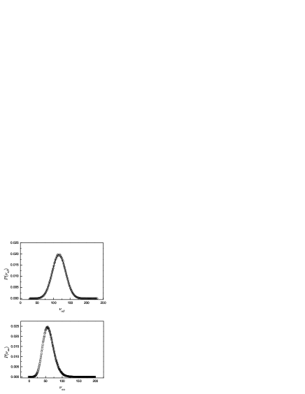
Figure 5: Probability distributions of $\nu_{\alpha\alpha}$ and $\nu_{\alpha\beta}$ in the metallic regime ($\langle g\rangle=2.52$) for a disorder of $w=0.2$. The solid lines correspond to a gaussian distribution for $\nu_{\alpha\beta}$ and a log-normal tail distribution for $\nu_{\alpha\alpha}$.

With increasing the disorder $w$, when we almost are in crossover regime we obtain a wide range variety of broad distributions as shown in Fig. 6 where we plot DF for two values of disorder: $w=0.5$ ($L/\xi=0.69$ and $\langle g\rangle=0.75$) in the left panel and $w=0.6$ ($L/\xi=0.93$ and $\langle g\rangle=0.5$) in the right panel. As one can see from Fig.6 (right panel) $P(\nu_{\alpha\beta})$ has a flat part for almost in all the range of $\nu_{\alpha\beta}$ while in the left panel it has a strong decay. In both cases the distributions for $P(\nu_{\alpha\beta})$ can be fitted to two log-normal tails. This type of behavior is typical also for distribution of conductance $g$ in the same range of parameters in Q1D, as one can see from the same Fig.6 where we present $P(g)$. For values $g<1$ we have a plat part while in the regime $g>1$ we get for distribution of conductance a strong decay. This is in complete agreement with a number of numerical simulation in the intermediate regime (see e.g. Ruhlanderal01 ; Ruhlandersoukoulis01 ; Gopar02 ).

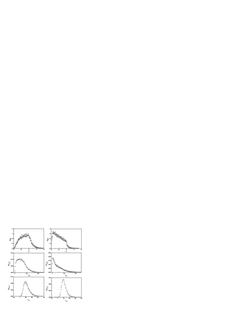
Figure 6: Distributions $P(g)$, $P(\nu_{\alpha\alpha})$ and $P(\nu_{\alpha\beta})$ in the crossover regime for two value of the disorder: right panel $w=0.5$ ($L/\xi=0.69$ and $\langle g\rangle=0.75$) and left panel $w=0.6$ ($L/\xi=0.93$ and $\langle g\rangle=0.5$).

As for $P(\nu_{\alpha\alpha})$ it is shifted to right, to much larger value of $\nu_{\alpha\alpha}$, which means that it becomes less conductive. For this range of parameters DF is still quite symmetric (right panel) but more wider if we compare with the DF from the Fig.5. The $P(\nu_{\alpha\alpha})$ for $w=0.6$ becomes less symmetric (left panel).

Further increase of the disorder $w$ (in the insulating region) $P(\nu_{\alpha\beta})$ becomes a one-side log-normal distribution. This type of behavior was predicted for distribution of conductance $g$ in Muttalib99 ; Gopar02 and numerically calculated in Ruhlanderal01 ; Ruhlandersoukoulis01 ; Garcia01 .

With regard to $P(\nu_{\alpha\alpha})$, we can mention that the tail of the distribution follows a power-law decay $P(\nu_{\alpha\alpha})\propto 1/\nu_{\alpha\alpha}^{m}$, with $m\simeq 2.3$. On the other hand, as $w$ increases $P(\nu_{\alpha\beta})$ shows a tail in the negative region of $\nu_{\alpha\beta}$. In Fig.7 we plot the distribution $P(\nu_{\alpha\alpha})$ and $P(\nu_{\alpha\beta})$ for a disorder $w=1$ ($L/\xi=2.6$ and $\langle g\rangle=0.08$).

Deeply in the localized regime ($L\gg\xi$ and $\langle g\rangle\approx 0$) the distribution of $\nu_{\alpha\beta}$ is log-normal as one can from Fig.8 where we fit $P(\ln\nu_{\alpha\beta})$ to a Gaussian distribution:

$$P(x)=\frac{B}{\sqrt{2\pi}\sigma x}e^{-{(\ln x-\mu)^{2}}/{2\sigma^{2}}},$$ (31)

with $B=0.997$, $\mu=-460.5$ and $\sigma=27.7$.

The shape of $P(\nu_{\alpha\alpha})$ is highly asymmetric with two peaks very closed each other. The position and the high of this peaks depend on the disorder parameter and cause several shapes of the distribution function. The tail of the distribution follows a power-law decay $P(\nu_{\alpha\alpha})\propto 1/\nu_{\alpha\alpha}^{m}$, with $m\simeq 2.0$

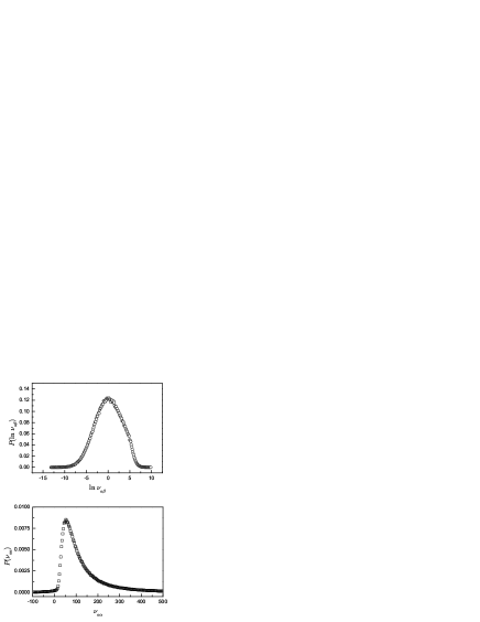
Figure 7: Distributions $P(\nu_{\alpha\alpha})$ and $P(\ln\nu_{\alpha\beta})$ in the insulating regime ($\langle g\rangle=0.08$) for a disorder of $W=1$. We have a one-side log-normal distribution for $\nu_{\alpha\beta}$ and power-law tail for $\nu_{\alpha\alpha}$, $P(\nu_{\alpha\alpha})\propto 1/\nu_{\alpha\alpha}^{m}$, with $m\simeq 2.3$

.

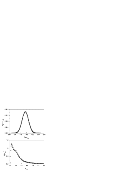
Figure 8: Distributions $P(\nu_{\alpha\alpha})$ and $P(\ln\nu_{\alpha\beta})$ in the insulating regime ($\langle g\rangle\approx 0$) for a disorder of $W=12$. The solid lines correspond to a gaussian distribution for $\ln\nu_{\alpha\beta}$ that point out a log-normal distribution for $\nu_{\alpha\beta}$. The tail of the distribution follows a power-law decay $P(\nu_{\alpha\alpha})\propto 1/\nu_{\alpha\alpha}^{m}$, with $m\simeq 2.0$

V Conclusions

We study the distributions functions for global partial density of states in quasi-one-dimensional disordered wires as a function of disorder parameter from metal to insulator. We consider two different models for disordered Q1D wire: a set of two dimensional $\delta$ potentials with an arbitrary signs and strengths placed randomly, and a tight-binding Hamiltonian with several modes and on-site disorder. It was shown that the poles of Green functions can be presented as determinant of the rank $N\times N$, where $N$ is the number of scatters. We show that the variances of partial global partial density of states in the metal to insulator crossover regime are crossing. The critical value of disorder $w_{c}$ where we have crossover can be used for calculation a localization length in Q1D systems. With increasing the numbers of mode the crossing point moves to the left and the $w_{c}$ decreases.

In the metallic regime when the system size much smaller than the localization length $L<<\xi$ the distribution function for $P(\nu_{\alpha\beta})$ is Gaussian-like. In the same regime the distribution function of $P(\nu_{\alpha\alpha})$ is include big range of negative $\nu_{\alpha\alpha}$ values indicating a predominantly inductive dynamic response of the system to an external ac electric field according BC98 . For positive values of $\nu_{\alpha\alpha}$ the tail of the distribution $P(\nu_{\alpha\alpha})$ is fairly log-normal. Almost in crossover regime the distribution function for $P(\nu_{\alpha\beta})$ can be fitted to two log-normal tails. As for $P(\nu_{\alpha\alpha})$ it is shifted to right, to much larger value of $\nu_{\alpha\alpha}$, which means that it becomes less conductive. Further increase of the disorder $w$ (in the insulating region) $P(\nu_{\alpha\beta})$ becomes a one-side log-normal distribution. With regard to $P(\nu_{\alpha\alpha})$, we can mention that the tail of the distribution follows a power-law decay $P(\nu_{\alpha\alpha})\propto 1/\nu_{\alpha\alpha}^{m}$, with $m\simeq 2.3$. Deeply in the localized regime ($L\gg\xi$ and $\langle g\rangle\approx 0$) the distribution of $\nu_{\alpha\beta}$ is log-normal and while the shape of $P(\nu_{\alpha\alpha})$ is highly asymmetric with two peaks very closed each other. The position and the high of this peaks depend on the disorder parameter and cause several shapes of the distribution function.

VI Acknowledgments

One of the authors (V.G.) thanks M. Büttiker for useful discussions and acknowledges the kind hospitality extended to him at the Murcia and Geneva Universities. J. R. thanks the FEDER and the Spanish DGI for financial support through Project No. FIS2004-03117.

VII Appendix: Dyson equation in Q1D disordered system and the poles of Green’s Function

We consider the Q1D wire with the impurities potential of the form:

$$V(x,y)=\sum_{n=1}^{N}V_{n}\delta(x-x_{n})\delta(y-y_{n}),$$ (32)

where $V_{n}$, $x_{n}$ and $y_{n}$ are arbitrary parameters. The equation for the Green function with above potential $V(x,y)$ is:

$$\left\{E-\left[-\frac{\hbar^{2}}{2m}\left(\frac{d^{2}}{dx^{2}}+\frac{d^{2}}{dy^{2}}\right)+V_{c}(y)+V(x,y)\right]\right\}G(xy;x^{\prime}y^{\prime})=\delta(x-x^{\prime})\delta(y-y^{\prime}),$$ (33)

where the confinement potential $V_{c}(y)$ depends only on the transverse direction $y$. The Dyson equation for a Q1D wire can be written in the form bagwell90 :

$$G_{ac}(x,x^{\prime})=G_{a}^{0}(x,x^{\prime})\delta_{ac}+\sum_{b,d}\int G_{a}^{0}(x,x^{\prime\prime})\delta_{ab}V_{bd}(x^{\prime\prime})G_{dc}(x^{\prime\prime},x^{\prime})\,dx^{\prime\prime},$$ (34)

The matrix $V_{ab}(x)$ elements of the defect potential are:

$$V_{ab}(x)=\int\chi_{a}^{\ast}(y)V(x,y)\chi_{b}(y)\,dy=\sum_{n=1}^{N}V_{ab}^{(n)}\delta(x-x_{n}),$$ (35)

and $V_{ab}^{(n)}$ defined as:

$$V_{ab}(x)=\chi_{a}^{\ast}(y_{n})V_{n}\chi_{b}(y_{n})\$$ (36)

Details on the calculation of the GF $G_{nm}(x,x^{\prime})$ of Dyson equation (33) for this case, based on the method developed in GA88 ; AG91 will be done elsewhere RG06 . Here we present main results of calculation which will be used in numerical calculations. The pole of GF can be rewritten as a determinant of the rank ($MN\times MN$) ($M$ is the number of modes and $N$ is the number of delta potentials) The matrix elements of determinant’s $(D_{MN})_{ln}$ are:

$$(D_{MN})_{nl}=-\mathit{I}\delta_{nl}+(\mathit{I}-\delta_{nl})\{\lambda_{nl}\}\{r^{\left(l\right)}\}.$$ (37)

Here:

$$\mathit{I}=\left(\begin{array}[]{ccc}1&\ldots&0\\ \vdots&\ddots&\vdots\\ 0&\ldots&1\end{array}\right)$$ (38)

is unit matrix. The $l$th scattering matrix $\{r^{\left(l\right)}\}$ and $\{\lambda_{nl}\}$ matrix are matrices $M\times M$ and defined in the following way:

$$\{r^{\left(l\right)}\}=\left(\begin{array}[]{ccc}r_{11}^{\left(l\right)}&\cdots&r_{1M}^{\left(l\right)}\\ \vdots&\ddots&\vdots\\ r_{M1}^{\left(l\right)}&\cdots&r_{MM}^{\left(l\right)}\end{array}\right),$$ (39)

$$\{\lambda_{nl}\}=\left(\begin{array}[]{ccc}\lambda^{(1)}_{nl}&\ldots&0\\ \vdots&\ddots&\vdots\\ 0&\cdots&\lambda^{(M)}_{nl}\end{array}\right)=\left(\begin{array}[]{ccc}e^{ik_{1}|x_{n}-x_{l}|}&\ldots&0\\ \vdots&\ddots&\vdots\\ 0&\cdots&e^{ik_{M}|x_{n}-x_{l}|}\end{array}\right),$$ (40)

The quantities $r_{mm}^{(l)}$ and $r_{km}^{(l)}$ are:

$$r_{mm}^{(l)}={\frac{V_{mm}^{(l)}G_{m}^{0}(x_{l},x_{l})}{1-\sum_{n}^{M}V_{nn}^{(l)}G_{n}^{0}(x_{l},x_{l})}}$$ (41)

$$r_{km}^{(l)}={\frac{V_{km}^{(l)}\sqrt{G_{k}^{0}(x_{l},x_{l})G_{m}^{0}(x_{l},x_{l})}}{1-\sum_{n}^{M}V_{nn}^{(l)}G_{n}^{0}(x_{l},x_{l})}}$$ (42)

respectively. $r_{mm}^{(l)}$ ($m=1,2,...M$) is the complex amplitude of the reflection of an electron from the isolate potential $V_{l}$ with the coordinates ${x_{l},y_{l}}$. Electron incidents from the normal mode $m$ on the left (right) and reflected normal mode $m$ on the left (right). $r_{km}^{(l)}$ is the complex reflection amplitude of an electron from the same $V_{l}$ but it incidents from the normal mode $m$ on the left (right) side and reflected normal mode $k$ on the same side: By permuting indexes $k$ and $m$ in (42) one can find the complex amplitude $r_{mk}^{(l)}$. Note that determinant of the matrix ${r^{(l)}}$ is zero, i.e.

$$det\{r^{\left(l\right)}\}=0.$$ (43)

This is follows from the fact that

$$r_{mm}^{\left(l\right)}r_{kk}^{\left(l\right)}-r_{mk}^{\left(l\right)}r_{km}^{\left(l\right)}=0,$$

which can be checked directly if one used the definitions of (42) and (41). The rank ($MN\times MN$) of the above determinant (see (37)), after some mathematical manipulation can be reduced to the determinant of the rank ($N\times N$), as in the case of 1D chain of arbitrary arranged potentials GA88 ; AG91 , with the following matrix elements:

$$(D_{N})_{nl}=-\delta_{nl}+(1-\delta_{nl})\left[r_{11}^{\left(l\right)}\lambda_{nl}^{\left(1\right)}+{\frac{1}{r_{11}^{\left(1\right)}}}\sum_{p=2}^{M}r_{1p}^{\left(1\right)}r_{p1}^{\left(p\right)}\lambda_{nl}^{\left(p\right)}\right].$$ (44)

Once we know the explicit form of $(D_{N})_{nl}$, we can calculate the scattering matrix elements without determining the exact electron wave function in disordered Q1D wire. For example the transmission amplitude $T_{11}^{(N)}$ from the set of $N$ delta potentials is:

$$T_{11}^{(N)}=e^{ik_{1}|x_{N}-x_{1}|}\frac{(\bar{D}_{N})_{nl}}{(D_{N})_{nl}}.$$ (45)

where the matrix $(\bar{D}_{N})_{nl}$ is obtained from the matrix $({D}_{N})_{nl}$ (Eq. (44)) by augmenting it on the left and on the top in the following way:

$$(\bar{D}_{N})_{nl}=\left|\begin{array}[]{cccc}1&r_{11}^{\left(l\right)}&\ldots&r_{11}^{\left(N\right)}e^{ik_{1}|x_{N}-x_{1}|}\\ 1&\ldots&\ldots&\ldots\\ \vdots&\vdots&(D_{N})_{nl}&\\ e^{-ik_{1}|x_{N}-x_{1}|}&\vdots&&\end{array}\right|.$$ (46)

The reflection amplitude $R_{11}^{(N)}$ of electrons from the same set of $N$ delta potentials is given by:

$$R_{11}^{(N)}=\frac{(\tilde{D}_{N})_{nl}}{(D_{N})_{nl}}.$$ (47)

where the matrix $(\tilde{D}_{N})_{nl}$ is obtained from the matrix $({D}_{N})_{nl}$ (Eq. (44)) by augmenting it on the left and on the top:

$$(\bar{D}_{N})_{nl}=\left|\begin{array}[]{cccc}0&r_{11}^{\left(l\right)}&\ldots&r_{11}^{\left(N\right)}e^{ik_{1}|x_{N}-x_{1}|}\\ 1&\ldots&\ldots&\ldots\\ \vdots&\vdots&(D_{N})_{nl}&\\ e^{ik_{1}|x_{N}-x_{1}|}&\vdots&&\end{array}\right|.$$ (48)

It can checked directly that Eq. (45) for the case of two point scatterers (i.e. $N=2$) and for two modes ($M=2$) lead us to ($a_{1}=x_{2}-x_{1}$)

$$T_{11}=e^{ik_{1}a_{1}}\frac{(1+r_{11}^{(1)})(1+r_{11}^{(2)})+r_{12}^{(1)}r_{21}^{(2)}e^{i(k_{2}-k_{1})a_{1}}-r_{22}^{(1)}r_{22}^{(2)}e^{2ik_{2}a_{1}}-e^{i(k_{1}+k_{2})a_{1}}r_{12}^{(2)}r_{21}^{(1)}}{1-r_{11}^{(1)}r_{11}^{(2)}e^{2ik_{1}a_{1}}-r_{22}^{(1)}r_{22}^{(2)}e^{2ik_{2}a_{1}}-\left(r_{12}^{(1)}r_{21}^{(2)}+r_{21}^{(1)}r_{12}^{(2)}\right)e^{i(k_{1}+k_{2})a_{1}}}$$

which, after appropriate notation used in Kumar91 , will coincides with their expression of $T_{11}$ calculated by transfer matrix method.

For $R_{11}^{(N)}$ from Eq. (47) we will get

$$R_{11}=\frac{r_{11}^{(1)}+r_{11}^{(2)}(1+2r_{11}^{(1)})e^{2ik_{1}a_{1}}+\left(r_{12}^{(1)}r_{21}^{(2)}+r_{21}^{(1)}r_{12}^{(2)}\right)e^{i(k_{1}+k_{2})a_{1}}}{1-r_{11}^{(1)}r_{11}^{(2)}e^{2ik_{1}a_{1}}-r_{22}^{(1)}r_{22}^{(2)}e^{2ik_{2}a_{1}}-\left(r_{12}^{(1)}r_{21}^{(2)}+r_{21}^{(1)}r_{12}^{(2)}\right)e^{i(k_{1}+k_{2})a_{1}}}$$

To close this section let us note that to get the expressions for the pole of the GF Eq. (37), for transmission amplitude $T_{11}^{(N)}$ and for $R_{11}^{(N)}$ in tight-binding model one must to replace the unperturbed GF for normal mode $m$

$$G_{m}^{0}(x,x^{\prime})=-i{\frac{m_{0}}{\hbar^{2}k_{m}}}\exp\left(ik_{a}|x-x^{\prime}|\right)$$ (49)

with

$$k_{m}=+\sqrt{\frac{2m_{0}(E-E_{m})}{\hbar^{2}}}$$ (50)

by the appropriate GF for tight-binding model Economou83 :

$$G_{m}^{0}(l,n)=-\frac{i}{\sqrt{B^{2}-(E-\epsilon)^{2}}}e^{|l-n|\Theta}$$ (51)

Here ($x\equiv(E-\epsilon)/B$)

$$\Theta=\ln(x-i\sqrt{1-x^{2}})$$ (52)

and symbol $\sqrt{1-x^{2}}$ denotes the positive square roots.

References

- (1) M. Büttiker, J. Phys.: Condensed Mater 5 9361 (1993).
- (2) M. Büttiker, H. Thomas and A. Prêtre, Z. Phys. B 94 133 (1994).
- (3) M. Brandbyge and M. Tsukada, Phys. Rev. B 57 15088 (1998).
- (4) Q. Zheng, J. Wang and H. Guo, Phys. Rev. B 56 12462 (1997).
- (5) V. Gasparian, T. Christen and M. Büttiker, Phys. Rev. A 54 4022 (1996).
- (6) M. Büttiker, Lecture Notes in Physics (Springer Verlag. Berlin, 2002).
- (7) H. Schomerus, M. Titov, P.W. Brouwer and C.W.J. Beenakker, Phys. Rev. B 65 R121101 (2002).
- (8) M. Büttiker and Pramana, J. Phys. 58 241 (2002).
- (9) M. Switkes, C.M. Marcus, K. Campman, A.C. Gossard, Science 283, 1905-1908,(1999).
- (10) P.W. Brouwer, Phys. Rev. B, 58, R10135-R10138, (1998).
- (11) M. Moskalets and M. Büttiker, Phys. Rev. B 66 035306 (2002).
- (12) C.J. Bolton-Heaton, C.J.Lambert, V.I.Falko, V.Prigodin and A.J. Epshtein Phys. Rev. B 60 10569 (1999).
- (13) M. Büttiker and T. Christen, in Theory of Transport Properties of Semiconductor Nanostructures, edited by E. Schöl (Chapman and Hall, London, 1998), pp. 215-248.
- (14) T. de Jesus, H. Guo, and J. Wang, Phys. Rev. B 62 10774 (2000).
- (15) S. Datta, Electronic Transport in Mesoscopic Systems (Cambridge University Press, 1995).
- (16) R. Landauer, J. Phys., Condens. Matter, 1 8099 (1989).
- (17) The details and results will be presented elsewhere.
- (18) D.S. Fisher and P.A. Lee, Phys. Rev. B 23 6851 (1981).
- (19) A. MacKinnon, Z. Phys. B 59 (1985) 385.
- (20) J.A. Verges, Comput. Phys. Commun. 118 71 (1999).
- (21) E. Abrahams, P.W. Anderson, D.C. Licciardello, and T.V. Ramakrishnan, Phys. Rev. Lett. 42 673 (1979).
- (22) I. M. Lifshitz, S. A. Gredeskul, and L. A. Pastur. Introduction to the Theory of Disordered Systems (Wiley, New York, 1988).
- (23) V. Gasparian, and M. Pollak, Phys. Rev. B 47 2038 (1993).
- (24) C. Texier and A. Comtet, Phys. Rev. Lett. 82 4220 (1999).
- (25) J. Heinrichs, Phys. Rev. B 65 75112 (2002).
- (26) M. Büttiker, Phys. Rev. B 27, 6178 (1983).
- (27) C.R. Leavens and G.C. Aers, Solid St. Commun. 63, 1101 (1987).
- (28) V. A. Gopar, K. A. Muttalib and P. Wölfle, Phys. Rev. B 66 174204 (2002).
- (29) M. Rühländer, P. Markov and C. M. Soukoulis, Phys. Rev. B 64 193103 (2001).
- (30) M. Rüländer and C. M. Soukoulis, Phys. Rev. B 63 85103 (2001).
- (31) K. A. Muttalib and P. Wölfle, Phys. Rev. Lett. 83 3013 (1999).
- (32) A. Garc a-Mart n and J. J. S enz, Phys. Rev. Lett. 87 116603 (2001).
- (33) P.F. Bagwell, J. Phys.: Condense. Matter 2 6179 (1990)
- (34) V.M. Gasparian, B.L. Altshuler, A.G. Aronov, and Z. H. Kasamanian, Phys. Lett. A, 132, 201-205, (1988).
- (35) A. G. Aronov, V. Gasparian, and U. Gummich, J. Phys.: Condens. Matter 3, 3023-3039, (1991).
- (36) M. Aubert, N. Bessis, and G. Bessis, Phys. Rev. A 10 51 (1974).
- (37) A. Kumar and P.F. Bagwell, Phys. Rev. B 43 9012 (1991)
- (38) E.N. Economou Green’s Functions in Quantum Physics (Springer-Verlag. Berlin, 1983).