Landauer conductance and twisted boundary conditions for Dirac fermions in two space dimensions

Abstract

We apply the generating function technique developed by Nazarov to the computation of the density of transmission eigenvalues for a two-dimensional free massless Dirac fermion, which, e.g., underlies theoretical descriptions of graphene. By modeling ideal leads attached to the sample as a conformal invariant boundary condition, we relate the generating function for the density of transmission eigenvalues to the twisted chiral partition functions of fermionic ($c=1$) and bosonic ($c=-1$) conformal field theories. We also discuss the scaling behavior of the ac Kubo conductivity and compare its different dc limits with results obtained from the Landauer conductance. Finally, we show that the disorder averaged Einstein conductivity is an analytic function of the disorder strength, with vanishing first-order correction, for a tight-binding model on the honeycomb lattice with weak real-valued and nearest-neighbor random hopping.

I Introduction

The recent manufacture of a single atomic layer of graphite (graphene) has renewed interest in the transport properties of Dirac fermions propagating in two-dimensional space. Novoselov04 ; Novoselov05 ; Zhang05a ; Zhang05b Recent theoretical work includes, among many others, the computation of the Landauer conductance for a single massless Dirac fermion by Katsnelson in Ref. Katsnelson06, , as well as the computation of the Landauer conductance and of the Fano factor in Ref. Tworzydlo06, , confirming the result of Ref. Katsnelson06, and predicting sub-Poissonian shot noise.

The conductivity has long been known to be related to a twist of boundary conditions. Edwards71 This idea has been further developed by Nazarov who proposed a generating function for the density of transmission eigenvalues in quasi-one-dimensional disordered conductors. Nazarov94 ; Rejaei96 ; Brouwer96 With this formalism, Lamacraft, Simons, and Zirnbauer reproduced in Ref. Lamacraft04, (see also Ref. Altland05, ) nonperturbative results of Refs. unitary Q1D wire, ; Mudry99, ; Brouwer00, for the mean conductance and the density of transmission eigenvalues of quasi-one-dimensional disordered quantum wires for three symmetry classes of Anderson localization.

The purpose of this paper is to establish a connection between (i) the density of transmission eigenvalues of the noninteracting Dirac Hamiltonian describing the free (ballistic) propagation of a relativistic massless electron in two-dimensional space and (ii) twisted chiral partition functions of a combination (tensor product) of two conformal field theories (CFTs) with central charges $c=1$ and $c=-1$. In this way we provide a complementary method for calculating the Landauer conductance of a single massless Dirac fermion which agrees with the direct calculations of Refs. Katsnelson06, and Tworzydlo06, , while it might give us a powerful tool to account for the nonperturbative effects for certain types of disorder. This connection comes from the observation that ideal leads attached to the sample, which are necessary to define the Landauer conductance, can be replaced by a set of conformally invariant boundary conditions. That this is possible is a consequence of the “diffusive” nature of the ballistic Dirac transport, as epitomized by its sub-Poissonian shot noise, which in turn suggests an insensitivity to the modeling of ideal leads.

The transport properties of noninteracting Dirac fermions in two-dimensional space under ideal conditions, i.e., without the breaking of translation invariance by disorder, have also been discussed in terms of the Kubo formula. However, extracting the dc value of the conductivity from the Kubo formula, which depends on frequency $\omega$, temperature $1/\beta$, and smearing $\eta$ (imaginary part of the self-energy), is rather subtle, as it is known that the conductivity in the dc limit $(\omega,1/\beta,\eta)=(0,0,0)$ is sensitive to how one approaches the dc limit.Ludwig94 ; Fradkin86 ; Lee93 ; Shon98 ; Durst99 ; Gorbar02 ; Peres05 ; Cserti06 ; Ziegler07 There have been at least two known limiting procedures: The Einstein conductivity, defined by first taking the zero temperature and then the zero frequency limits while keeping $\eta$ finite, is given by $1/\pi$ in units of $e^{2}/h$.Ludwig94 ; Fradkin86 ; Lee93 ; Shon98 ; Durst99 ; Gorbar02 ; Peres05 ; Cserti06 ; Ziegler07 On the other hand, by switching the order of zero smearing and zero frequency limits, one obtains, instead, $\pi/8$ for the dc conductivity (again in units of $e^{2}/h$).Ludwig94 ; Cserti06

To clarify the origin of this sensitivity to how the dc limit is taken, we compute the ac Kubo conductivity without taking any biased limit in $\omega$, $1/\beta$, or $\eta$. Due to the scale invariance of noninteracting Dirac fermions, we show the Kubo conductivity to be a scaling function of two scaling variables. We discuss several limiting procedures, including the above two, and clarify the relationship between different dc values. In particular, we demonstrate that, if we take the zero smearing limit prior to the other two limits, we can obtain any value between 0 and $\pi/8$ for the dc Kubo conductivity. The Einstein conductivity agrees with the conductivity determined from the Landauer conductance. We also compute several asymptotic behaviors of the Kubo conductivity that have not been obtained before. These considerations may be of relevance to experiments on graphene if different limiting procedures are accessed.

The perturbative effects of disorder in the form of weak real-valued random (white-noise) hopping between nearest-neighbor sites of the honeycomb lattice at the band center are discussed. We show that, as a consequence of the fixed point theory discussed in Ref. Guruswamy00, , the Einstein conductivity is an analytic function of the disorder strength. We also show that the first-order correction to the Einstein conductivity vanishes, in agreement with a calculation performed by Ostrovsky et al. in Ref. Ostrovsky06, . This result is of relevance to the two-dimensional chiral-orthogonal universality class.Verbaarschot94 ; Zirnbauer96 ; Altland97 ; Heinzner05 Potential relationships of the two-dimensional chiral symmetry class with certain types of disorder in graphene were recently discussed in Ref.  Ostrovsky06, . We refer the reader to Refs. Ostrovsky06, , Aleiner06, , and Altland06, for a discussion of white-noise disorder in graphene in terms of symmetry classes and to Refs. Aleiner06, ; Altland06, ; Ando02, ; Rycerz07, ; Nomura07, for the possibility that smooth disorder could induce crossovers between different symmetry classes.

II Model

Our starting point is the single-species (or one-flavor) Dirac Hamiltonian

$$\begin{split}\mathcal{H}:=-{i}\hbar v^{\ }_{F}\,\sigma^{\ }_{\mu}\,\partial^{\ }_{\mu},\qquad\hat{H}:=\int d^{2}r\,\hat{\Psi}^{{\dagger}}\mathcal{H}\hat{\Psi}^{\ },\end{split}$$ (1)

where $\hat{\Psi}^{{\dagger}}$ ($\hat{\Psi}$) is a two-component fermionic creation (annihilation) operator and $v^{\ }_{F}$ the Fermi velocity. We choose $\sigma^{\ }_{\mu=x,y}$ to be the first two of the three Pauli matrices $\sigma^{\ }_{x}$, $\sigma^{\ }_{y}$, and $\sigma^{\ }_{z}$ in the standard representation. (We use the summation convention over repeated indices.) Hamiltonian (1) describes the free relativistic propagation of a spinless fermion in two-dimensional space parametrized by the coordinates $r=(x,y)$. As such, it possesses the chiral symmetry

$$\sigma^{\ }_{z}\,\mathcal{H}\,\sigma^{\ }_{z}=-\mathcal{H}.$$ (2)

The single-particle retarded and advanced Green’s functions are defined by

$$\mathcal{G}^{{R}/{A}}_{\eta}(\varepsilon):=(\varepsilon\pm{i}\hbar\eta-\mathcal{H})^{-1}.$$ (3)

Consequently, at the band center $\varepsilon=0$, they are related to each other by the chiral transformation as

$$\sigma^{\ }_{z}\,\mathcal{G}^{{R}}_{\eta}(\varepsilon=0)\,\sigma^{\ }_{z}=-\mathcal{G}^{{A}}_{\eta}(\varepsilon=0).$$ (4)

Below, matrix elements between eigenstates of the position operator of the single-particle retarded Green’s function evaluated at $\varepsilon$ are denoted by $\mathcal{G}^{{R}}_{\eta}(r,r^{\prime};\varepsilon)$.

In the presence of an electromagnetic vector potential $A^{\ }_{\mu}(r)$, one modifies Hamiltonian (1) through the minimal coupling $\partial^{\ }_{\mu}\to\partial^{\ }_{\mu}-{i}(e/\hbar c)A^{\ }_{\mu}$ (with $e<0$). The conserved charge current then follows from taking the functional derivative with respect to $A^{\ }_{\mu}(r)$,

$$\begin{split}\hat{j}^{\ }_{\mu}(r)=\left(\hat{\Psi}^{{\dagger}}j^{\ }_{\mu}\hat{\Psi}\right)(r),\qquad j^{\ }_{\mu}&:=ev^{\ }_{F}\,\sigma^{\ }_{\mu}.\end{split}$$ (5)

There is no diamagnetic contribution due to the linear dispersion.

III Kubo and Einstein conductivities

III.1 Linear response

We start from the bilocal conductivity tensor at a finite temperature $1/\beta$ defined by the linear response relation in the frequency-$\omega$ domain

$$\begin{split}j^{\mathrm{ind}}_{\mu}(r,\omega,\beta)=&\int d^{2}r^{\prime}\,\sigma^{\ }_{\mu\nu}(r,r^{\prime};\omega,\delta,\beta)E^{\ }_{\nu}(r^{\prime},\omega)\end{split}$$ (6a)

between the $$\omega E^{\ }_{\nu}(r^{\prime},\omega) t=-\infty j^{\mathrm{ind}}_{\mu}(r,\omega,\beta)$$ component of an electric field that has been switched on adiabatically at and the induced local current , where Mahan

$$\sigma^{\ }_{\mu\nu}(r,r^{\prime};\omega,\delta,\beta)=\frac{D^{{R}}_{\mu\nu}(r,r^{\prime};\omega,\delta,\beta)}{\hbar\omega}.$$ (6b)

Here,

$$D^{{R}}_{\mu\nu}(r,r^{\prime};\omega,\delta,\beta):=\int\limits_{0}^{\infty}\!dt\,e^{\mathrm{i}(\omega+{i}\delta)t}\left\langle\big{[}\hat{j}^{\ }_{\mu}(r,t),\hat{j}^{\ }_{\nu}(r^{\prime})\big{]}\right\rangle^{\ }_{\beta}$$ (6c)

is the response function, $\hat{j}_{\mu}(r,t)$ is the current operator in the Heisenberg picture, and $\langle\cdots\rangle^{\ }_{\beta}$ is the expectation value taken with respect to the equilibrium density matrix at temperature $1/\beta$. The small positive number $\delta>0$ implements the adiabatic switch-on of the electric field. The conductivity tensor in a sample of linear size $L$ is defined by integrating over the spatial coordinates of the bilocal conductivity tensor,

$$\sigma^{\ }_{\mu\nu}(\omega,\delta,\beta,L):=\int\frac{d^{2}r}{L^{2}}\int d^{2}r^{\prime}\sigma^{\ }_{\mu\nu}(r,r^{\prime};\omega,\delta,\beta).$$ (7)

We impose periodic boundary conditions and choose to represent the Dirac Hamiltonian (1) by

$$\hat{H}=\sum_{p}\sum_{\sigma=\pm}\sigma\varepsilon^{\ }_{p}\hat{a}^{{\dagger}}_{p,\sigma}\hat{a}^{\ }_{p,\sigma},$$ (8a)

where the fermionic creation operators $$\hat{a}^{{\dagger}}_{p,\sigma} \sigma=\pm |0\rangle p^{\ }_{\mu}$$ with create from the Fock vacuum the single-particle eigenstates with momentum

$$|m\rangle\equiv|p,\sigma\rangle\equiv\hat{a}^{{\dagger}}_{p,\sigma}|0\rangle:=\frac{1}{\sqrt{2}|p|}\left(\begin{array}[]{c}\sigma\left(p^{\ }_{x}-{i}p^{\ }_{y}\right)\\ |p|\end{array}\right),$$ (8b)

of $$\mathcal{H} \varepsilon^{\ }_{m}$$ with the single-particle energy eigenvalues ,

$$\varepsilon^{\ }_{m}\equiv\sigma\varepsilon^{\ }_{p}=\sigma v^{\ }_{F}|p|\equiv\sigma v^{\ }_{F}\sqrt{p^{2}_{x}+p^{2}_{y}}.$$ (8c)

The conductivity tensor can then be expressed solely in terms of single-particle plane waves

$$\begin{split}\sigma^{\ }_{\mu\nu}(\omega,\delta,\beta,L)=&\,\frac{{i}}{\omega}\int d\varepsilon\,\int\frac{d^{2}r}{L^{2}}\int d^{2}r^{\prime}\\ &\times\sum_{m,n}\langle m|\hat{j}^{\ }_{\mu}(r)|n\rangle\langle n|\hat{j}^{\ }_{\nu}(r^{\prime})|m\rangle\\ &\times\delta(\varepsilon-\varepsilon^{\ }_{m})\frac{f^{\ }_{\beta}(\varepsilon)-f^{\ }_{\beta}(\varepsilon^{\ }_{n})}{\varepsilon-\varepsilon^{\ }_{n}+\hbar\left(\omega+{i}\delta\right)},\end{split}$$ (9)

where $f^{\ }_{\beta}(\varepsilon):=1/(e^{\beta\varepsilon}+1)$ is the Fermi-Dirac function at temperature $1/\beta$ and at zero chemical potential.

As usual, the infinite-volume limit $L\to\infty$ has to be taken before the $\delta\to 0$ limit in Eq. (9). (Recall that $\delta$ controls the adiabatic switching of the external field.) In the following, it is understood that we always take these limits prior to any other limits. We thus drop the explicit $\delta$ and $L$ dependence of the conductivity tensor henceforth. The dc conductivity can then be computed by taking the subsequent limit, $\omega\to 0$. The temperature $1/\beta$ can be fixed to some arbitrary value.

The real part of Eq. (9) can be further rewritten in terms of single-particle Green’s functions. This can be done by first replacing the two $\delta$ functions in the real part of Eq. (9), which appear after taking the $\delta\to 0$ limit, by two Lorentzians with the same width $\hbar\eta$ (see, for example, Ref. Baranger89, ). Then, each Lorentzian can be rewritten as the difference of the retarded and advanced Green’s functions, $\mathcal{G}^{R}_{\eta}(\varepsilon)-\mathcal{G}^{A}_{\eta}(\varepsilon)$. By also noting that the transverse components ($\mu\neq\nu$) of the conductivity tensor (9) vanish by the spatial symmetries of the matrix elements in $\int d^{2}r\int d^{2}r^{\prime}\langle m|\hat{j}^{\ }_{\mu}(r)|n\rangle\langle n|\hat{j}^{\ }_{\nu}(r^{\prime})|m\rangle$, we obtain

$$\begin{split}\mathrm{Re}\,\sigma^{\ }_{\mu\nu}(\omega,\eta,\beta)=&\,\delta^{\ }_{\mu\nu}\,\frac{\hbar}{4\pi}\int d\varepsilon\frac{f^{\ }_{\beta}(\varepsilon+\hbar\omega)-f_{\beta}(\varepsilon)}{\hbar\omega}\\ &\times\int\frac{d^{2}r}{L^{2}}\int d^{2}r^{\prime}\Sigma^{\ }_{\mu\nu}(r,r^{\prime};\varepsilon,\omega,\eta),\end{split}$$ (10)

where we have introduced

$$\begin{split}\Sigma^{\ }_{\mu\nu}(r,r^{\prime};\varepsilon,\omega,\eta):=&\,\mathrm{tr}\,\Big{[}\mathcal{G}^{{A}-{R}}_{\eta}(r^{\prime},r;\varepsilon)j^{\ }_{\mu}\\ &\times\mathcal{G}^{{A}-{R}}_{\eta}(r,r^{\prime};\varepsilon+\hbar\omega)j^{\ }_{\nu}\Big{]}\end{split}$$ (11)

and $j^{\ }_{\mu}$ is defined in Eqs. (5). Here the trace is taken over spinor indices and

$$\mathcal{G}^{{A}-{R}}_{\eta}(r,r^{\prime};\varepsilon):=\mathcal{G}^{{A}}_{\eta}(r,r^{\prime};\varepsilon)-\mathcal{G}^{{R}}_{\eta}(r,r^{\prime};\varepsilon).\$$ (12)

Using translational invariance, the single-particle Green’s functions are given byfootnote: a dot b

$$\begin{split}\mathcal{G}^{R/A}_{\eta}(r^{\ }_{1},r^{\ }_{2};\varepsilon)=&\int_{k}e^{+{i}k\cdot(r^{\ }_{2}-r^{\ }_{1})}\mathcal{G}^{R/A}_{\eta}(k;\varepsilon),\\ \mathcal{G}^{R/A}_{\eta}(k;\varepsilon)=&\frac{1}{\varepsilon\pm{i}\hbar\eta-\hbar v^{\ }_{F}k\cdot\sigma}.\end{split}$$ (13)

In order to define the conductivity in the clean system we should take the $\eta\to 0$ limit before the $\omega\to 0$ limit. On the other hand, $\eta$ can be interpreted physically as a finite inverse life time (imaginary part of the self energy) induced by disorder. Thus, it is meaningful to discuss Eq. (10) in the presence of finite $\eta$. Below, we first discuss the $\eta\to 0$ limit. We will then discuss the case of finite $\eta$.

III.2 $\eta\to 0$ limit

We define the ac Kubo conductivity tensor at any finite frequency $\omega>0$ and temperature $1/\beta$ by

$$\begin{split}\sigma^{\mathrm{K}}_{\mu\nu}(\omega,\beta):=&\lim_{\eta\to 0}\mathrm{Re}\,\sigma^{\ }_{\mu\nu}(\omega,\eta,\beta).\end{split}$$ (14)

With the help of Eq. (9),

$$\begin{split}\sigma^{\mathrm{K}}_{\mu\nu}(\omega,\beta)=&\frac{\pi(ev^{\ }_{F})^{2}}{\omega}\sum_{m,n}\langle m|\sigma^{\ }_{\mu}|n\rangle\langle n|\sigma^{\ }_{\nu}|m\rangle\\ &\times\left[f^{\ }_{\beta}(\varepsilon^{\ }_{m})-f^{\ }_{\beta}(\varepsilon^{\ }_{n})\right]\delta\left(\varepsilon^{\ }_{m}-\varepsilon^{\ }_{n}+\hbar\omega\right).\end{split}$$ (15)

When $\omega>0$ and $\beta<\infty$, the sum over the basis (8b) in the real part of Eq. (15) can be performed once the matrix elements of the currents have been evaluated, yielding

$$\sigma^{\mathrm{K}}_{\mu\nu}(\omega,\beta) = \delta^{\ }_{\mu\nu}\frac{e^{2}}{h}\frac{\pi}{8}\tanh\frac{\beta\hbar\omega}{4}.$$ (16)

Observe that Eq. (16) is independent of the Fermi velocity $v^{\ }_{F}$.footnote: role of zero modes Finally, the ac Kubo conductivity (16) depends solely on the combination

$$Z:=\beta\hbar\omega\in\mathbb{R}.$$ (17)

The limiting value of Eq. (16) when $\omega\to 0$ and $\beta\to\infty$ can be any number between 0 and $e^{2}\pi/(8h)$ provided the scaling variable (17) is held fixed. For example, if the limit $\beta\to\infty$ is taken before the limit $\omega\to 0$, then

$$\lim_{\omega\to 0}\lim_{\beta\to\infty}\sigma^{\mathrm{K}}_{\mu\nu}(\omega,\beta)=\delta^{\ }_{\mu\nu}\frac{e^{2}}{h}\frac{\pi}{8}.$$ (18)

This limiting procedure reproduces the results from Refs. Ludwig94, and Cserti06, . On the other hand, if the limit $\omega\to 0$ is taken before the limit $\beta\to 0$, then

$$\lim_{\beta\to\infty}\lim_{\omega\to 0}\sigma^{\mathrm{K}}_{\mu\nu}(\omega,\beta)=0.$$ (19)

Clearly, $\lim_{\beta\to\infty}\sigma^{\mathrm{K}}_{\mu\nu}(\omega,\beta)=\delta^{\ }_{\mu\nu}(\pi/8)(e^{2}/h)$ for any finite frequency $\omega$, while $\lim_{\omega\to 0}\sigma^{\mathrm{K}}_{\mu\nu}(\omega,\beta)=0$ for any finite temperature $1/\beta$. The singularity at $\omega=1/\beta=0$ is a manifestation of the linear dispersion of the massless Dirac spectrum leading to a dependence on the scaled variables $\omega$ and $\beta$.

III.3 Case of finite $\eta>0$

For $\eta$ finite, it is shown in Appendix A that the real part of the longitudinal conductivity, Eq. (10), is a scaling function of two variables, i.e.,

$$\mathrm{Re}\,\sigma^{\ }_{xx}(\omega,\eta,\beta)=\mathrm{Re}\,\sigma^{\ }_{xx}(X,Y),$$ (20)

where

$$X:=\frac{\omega}{\eta},\qquad Y:=\frac{1}{\beta\hbar\eta}.$$ (21)

III.3.1 dc response $\omega=0$

If we take the dc limit $\omega\to 0$ while keeping $\eta>0$ finite, Eq. (10) can be expressed as

$$\begin{split}\mathrm{Re}\,\sigma^{\ }_{\mu\nu}(X=0,Y)=&\,\delta^{\ }_{\mu\nu}\frac{\hbar}{4\pi}\int d\varepsilon\frac{\partial f^{\ }_{\beta}}{\partial\varepsilon}\int\frac{d^{2}r}{L^{2}}\int d^{2}r^{\prime}\\ &\times\Sigma^{\ }_{\mu\nu}(r,r^{\prime};\varepsilon,\omega=0,\eta),\end{split}$$ (22)

where $\Sigma^{\ }_{\mu\nu}$ is defined in Eqs. (11) and (12). With the help of [see Eqs. (1) and (5)]

$$j^{\ }_{\mu}={i}e\left[\mathcal{H},r^{\ }_{\mu}\right]/\hbar,$$ (23)

one can show that Kramer93

$$\begin{split}\mathrm{Re}\,\sigma^{\ }_{\mu\nu}(X=0,Y)=&\,\delta^{\ }_{\mu\nu}\frac{e^{2}}{h}\eta^{2}\int d\varepsilon\frac{\partial f_{\beta}}{\partial\varepsilon}\int d^{2}r\,r^{2}\,\\ &\times\mathrm{tr}\,\left[\mathcal{G}^{R}_{\eta}(0,r;\varepsilon)\mathcal{G}^{A}_{\eta}(r,0;\varepsilon)\right],\end{split}$$ (24)

with $\mu=x,y$. Equation (24) is usually referred to as the Einstein conductivity since it is related to the diffusion constant via the Einstein relation (see, for example, Ref. McKane81, ).

A closed-form expression for Eq. (22) can be obtained at zero temperature,

$$\mathrm{Re}\,\sigma^{\ }_{\mu\nu}(X=0,Y=0)=\delta^{\ }_{\mu\nu}\frac{e^{2}}{h}\frac{1}{\pi}.$$ (25)

The same value was derived in Ref. Ludwig94, . Related predictions were also made, among others, in Refs. Fradkin86, , Lee93, , Shon98, , Durst99, , Gorbar02, , Peres05, , and Cserti06, . footnote: Durst Equation (25) also agrees with the conductivity determined from the Landauer formula. (This was first observed in Ref. Katsnelson06, . We will reproduce this fact in Sec. IV from Nazarov’s generating function technique.)

Whenever $\eta>0$, Eq. (10) is an analytic function of $X$ and $Y$ at $(X,Y)=(0,0)$. For $X,Y\ll 1$, the power series expansion of Eq. (10) in terms of $X$ and $Y$ is given by

$$\begin{split}\mathrm{Re}\,\sigma^{\ }_{xx}(X\ll 1,Y\ll 1)=\frac{e^{2}}{h}\frac{1}{\pi}\left[1+\left(\frac{X}{3}\right)^{2}+\left(\frac{\pi Y}{3}\right)^{2}\right]\end{split}$$ (26)

up to terms of order $X^{4}$, $Y^{4}$, or $X^{2}Y^{2}$.

III.3.2 Arbitrary $\omega$ and $\beta$ at finite $\eta$

For generic values of $(X=\omega/\eta,Y=1/\beta\hbar\eta)$, we are unable to evaluate the real part of the longitudinal conductivity from Eq. (10) in closed form. The numerical integration of Eq. (10) when $\mu=\nu=x$ or, equivalently, of Eq. (87a) is presented in Fig. 1. OtherNumericsFigOne

First, we fix $Y=1/(\beta\hbar\eta)$ and discuss the $X=\omega/\eta$ dependence of the real part of the longitudinal conductivity from Eq. (10). We distinguish two limits. When $X\to\infty$ as happens when the frequency $\omega$ is much larger than the inverse life-time $\eta$, the real part of the longitudinal conductivity measured in units of $e^{2}/h$ converges to the limiting value $\pi/8$. In the opposite limit of $X\to 0$, the limiting value is an increasing function of $Y$ and is given by Eq. (26) with $X=0$, when the temperature $1/\beta$ is much smaller than the energy smearing $\hbar\eta$ ($Y\ll 1$). These two limiting behaviors are smoothly connected as is illustrated in Fig. 1(a). For example, $(h/e^{2})\,\mathrm{Re}\,\sigma^{\ }_{xx}(X,Y=0)$ increases monotonically between $1/\pi$ and $\pi/8$ as a function of $X$.Ostrovsky06 The approach to the limiting value $\pi/8$ for large $X$ when $Y=0$ is given by

$$\mathrm{Re}\,\sigma^{\ }_{xx}(X\gg 1,Y=0)=\frac{e^{2}}{h}\left(\frac{\pi}{8}-\frac{1}{3X^{3}}\right)$$ (27)

up to terms of order $X^{-4}$. For $Y\gg 1$ the approach to the limit $X\to 0$ is Drude-like,

$$\mathrm{Re}\,\sigma^{\ }_{xx}(X\ll 1,Y\gg 1)\sim\frac{e^{2}}{h}\frac{2Y\ln 2}{X^{2}+4}.$$ (28)

Second, we fix $X=\omega/\eta$ and discuss the $Y=1/(\beta\hbar\eta)$ dependence of the real part of the longitudinal conductivity from Eq. (10). When $Y\gg 1$ as happens when the temperature $\beta^{-1}$ is much larger than the energy resolution $\hbar\eta$, $(h/e^{2})\,\mathrm{Re}\,\sigma^{\ }_{xx}(X,Y)\sim gY$ for any fixed value of $X$ where $g$ is some constant. In particular, when $X=0$, we find

$$\mathrm{Re}\,\sigma^{\ }_{xx}(X=0,Y\gg 1)=\frac{e^{2}}{h}\frac{\ln 2}{2}\,Y$$ (29)

to leading order in $Y\gg 1$.Wallace47 ; Gorbar02 In the opposite limit of $Y\ll 1$, the conductivity approaches a finite value given by Eq. (26) with $Y=0$ when $X\ll 1$, which is thus an increasing function of $X\ll 1$ in agreement with Fig. 1(b). The dependence on $Y$ of $\mathrm{Re}\,\sigma^{\ }_{xx}(X,Y)$ is monotonic increasing if $X=0$ while it is nonmonotonic for the finite values of $X$ given in Fig. 1(b).

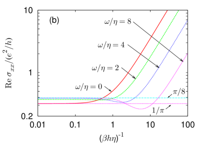
Figure 1: (Color online) Numerical integration of Eq. (10) when $\mu=\nu=x$ as a function of $X=\omega/\eta$ (a) and $Y=(\beta\hbar\eta)^{-1}$ (b). The dc limit $\omega/\eta=0$ in (b) is obtained from numerical integration of Eq. (22).

IV Landauer conductance

In this section we are going to reproduce the calculation of the Landauer conductance for a single massless Dirac fermion from Refs. Katsnelson06, and Tworzydlo06, using the tools of CFT subjected to boundary conditions that preserve conformal invariance. Although the direct methods of Refs. Katsnelson06, and Tworzydlo06, are both elegant and physically intuitive in the ballistic regime, we are hoping that the CFT approach might lend itself to a nonperturbative treatment of certain types of disorder.

IV.1 Definition

In order to define the Landauer conductance, we consider a finite region, the sample, described by the Dirac Hamiltonian, and attach a set of leads (or reservoirs) $l^{\ }_{1},l^{\ }_{2},\cdots$ to the sample. Propagation in the leads obeys different laws than in the sample. footnote: ideal leads Then, the (dimensionfull) conductance $G^{\mathrm{L}}_{a\to b}$ for the transport from the $a$th to $b$th lead is determined from the transmission matrix $T^{\ }_{a\to b}$ by

$$G^{\mathrm{L}}_{a\to b}:=\frac{e^{2}}{h}\mathrm{tr}^{\prime}\left(T^{{\dagger}}_{a\to b}T^{\ }_{a\to b}\right)$$ (30)

where $\mathrm{tr}^{\prime}$ denotes the trace over all channels in the $b$th lead. The Landauer conductance (30) can be expressed in terms of the bilocal conductivity tensor $\Sigma^{\ }_{\mu\nu}$ of Eq. (10), according to Fisher81 ; Baranger89 ; Xiong96

$$G^{\mathrm{L}}_{a\to b}=-\int_{a}\int_{b}dS^{\mu}_{a}dS^{\prime\nu}_{b}\,\Sigma^{\ }_{\mu\nu}(r,r^{\prime};\varepsilon=0,\omega=0,\eta=0),$$ (31)

where $r$ ($r^{\prime}$) is constrained to lie on the interface between the $a$th ($b$th) lead and the sample, and $\int_{a}dS^{\mu}_{a}$ represents integration over the oriented interface between the sample and the $a$th lead.

To define the longitudinal Landauer conductance we choose for the sample the surface of a cylinder of length $L^{\ }_{x}$ and of perimeter $L^{\ }_{y}$ to which we attach two ideal leads $l^{\ }_{1}$ and $l^{\ }_{2}$ at the left end $x^{\ }_{L}=-L^{\ }_{x}/2$ and right end $x^{\ }_{R}=+L^{\ }_{x}/2$, respectively.footnote: ideal leads

For the free Dirac Hamiltonian (1), the dimensionless conductance along the $x$ direction,

$$g^{\mathrm{L}}_{xx}=(h/e^{2})G^{\mathrm{L}}_{xx}\equiv(h/e^{2})G^{\mathrm{L}}_{1\to 2},$$ (32a)

can then be expressed in terms of the single-particle Green’s function of Eq. (3) as

$$\begin{split}g^{\mathrm{L}}_{xx}=&(\hbar v^{\ }_{F})^{2}\oint\limits^{0}_{L_{y}}dy\oint\limits^{L^{\ }_{y}}_{0}dy^{\prime}\,\\ &\times\mathrm{tr}\left[\mathcal{G}^{R}_{\eta=0}(r,r^{\prime};0)\sigma^{\ }_{+}\mathcal{G}^{R}_{\eta=0}(r^{\prime},r;0)\sigma^{\ }_{-}\right],\end{split}$$ (32b)

where $r=(x^{\ }_{L},y)$, $r^{\prime}=(x^{\ }_{R},y^{\prime})$, and $\sigma^{\ }_{\pm}=\sigma^{\ }_{x}\pm{i}\sigma^{\ }_{y}$. We made use of the chiral symmetry and of $\Sigma^{\ }_{\mu\mu}(r,r^{\prime};\varepsilon=0,\omega=0,\eta=0)=\Sigma^{\ }_{\mu\mu}(r^{\prime},r;\varepsilon=0,\omega=0,\eta=0)$. The single-particle Green’s functions that enter Eq. (31) are obtained by solving the Schrödinger equation for the entire system, including the leads. footnote: ideal leads For convenience, we assume that the leads also respect chiralVerbaarschot94 ; Zirnbauer96 ; Altland97 ; Heinzner05 symmetry. The imaginary part $\hbar\eta$ of the energy can be set to zero in the sample, since the ideal leads broaden the energy levels in the sample.

In the sequel, we will use Nazarov’s technique to derive the following expressions for the dimensionless conductance along the $x$ direction,

$$g^{\mathrm{L}}_{xx}=\frac{1}{\pi}\frac{L^{\ }_{y}}{L^{\ }_{x}}+\mathcal{O}[(L^{\ }_{y}/L^{\ }_{x})^{0}].$$ (33)

Thus, since the longitudinal conductivity $\sigma^{\ }_{xx}$ can be extracted from the conductance in the anisotropic limit via $g^{\mathrm{L}}_{xx}=\sigma^{\ }_{xx}L^{\ }_{y}/L^{\ }_{x}$ where $L^{\ }_{x}\ll L^{\ }_{y}$, we recover from (33) the result (25) for the longitudinal Kubo dc conductivity.

The transverse Landauer conductance $g^{\mathrm{L}}_{xy}$ can be defined by taking the sample to be a rectangular region $[-L^{\ }_{x}/2,+L^{\ }_{x}/2]\times[-L^{\ }_{y}/2,+L^{\ }_{y}/2]$ and attaching four ideal leads to each edge. As is the case for the Kubo conductivity, we are going to show that

$$g^{\mathrm{L}}_{xy}=0.$$ (34)

We now turn to the derivations of Eqs. (33) and (34) for which we shall set

$$\hbar=v^{\ }_{F}=-e=1$$ (35)

unless these constants are written explicitly.

IV.2 Nazarov formula

Following Refs. Nazarov94, ; Altland05, ; Rejaei96, ; Brouwer96, ; Lamacraft04, , we introduce the generating function for the transmission eigenvalue density

$${Z}(\theta^{\ }_{F},\theta^{\ }_{B}):=\frac{\mathrm{Det}\,\left(1-\gamma^{\ }_{L}\gamma^{\ }_{R}\hat{v}^{\ }_{L}\mathcal{G}^{R}_{\eta}(0)\hat{v}^{\ }_{R}\mathcal{G}^{R}_{\eta}(0)\right)}{\mathrm{Det}\,\left(1-\zeta^{\ }_{L}\zeta^{\ }_{R}\hat{v}^{\ }_{L}\mathcal{G}^{R}_{\eta}(0)\hat{v}^{\ }_{R}\mathcal{G}^{R}_{\eta}(0)\right)}.$$ (36)

Here, $\mathrm{Det}$ refers to the functional determinant over all spatial coordinates (both inside and outside of the sample) and spinor indices. We have also defined

$$\hat{v}^{\ }_{R/L} = {i}\sigma^{\ }_{\pm}\delta(x-x^{\ }_{R/L}).$$ (37)

Finally, the source terms are parametrized by $\theta_{F}$ and $\theta_{B}$ as

$$\begin{split}\gamma^{\ }_{R}=\tan\frac{\theta^{\ }_{F}}{2},\qquad\gamma^{\ }_{L}=\sin\frac{\theta^{\ }_{F}}{2}\cos\frac{\theta^{\ }_{F}}{2},\\ \zeta^{\ }_{R}=\tan\frac{{i}\theta^{\ }_{B}}{2},\qquad\zeta^{\ }_{L}=\sin\frac{{i}\theta^{\ }_{B}}{2}\cos\frac{{i}\theta^{\ }_{B}}{2}.\end{split}$$ (38)

The Landauer conductance is then given by

$$g^{\mathrm{L}}_{xx}=\left.\frac{\partial Z}{\partial\left(\gamma^{\ }_{L}\gamma^{\ }_{R}\right)}\right|^{\ }_{\gamma^{\ }_{L}\gamma^{\ }_{R}=\zeta^{\ }_{L}\zeta^{\ }_{R}=0}.$$ (39)

Furthermore, if the transmission probability $T^{\ }_{n}$ in channel $n$ (transmission eigenvalue), the $n$th positive real-valued eigenvalue of the product of transmission matrices entering Eq. (30) in descending order, is written as

$$T^{\ }_{n}=:\cosh^{-2}(\theta^{\ }_{n}/2),$$ (40)

then the density of transmission eigenvalues,

$$\rho(\theta):=\sum_{n}\delta(\theta-\theta^{\ }_{n}),$$ (41a)

is given by

$$\begin{split}\rho(\theta)=&\frac{1}{2\pi}\left[F(\theta+{i}0^{+}+{i}\pi)-F(\theta-{i}0^{+}-{i}\pi)\right],\\ F(\theta)=&\left.\frac{1}{2}\left(\frac{\partial}{\partial\theta^{\ }_{F}}-\frac{\partial}{{i}\partial\theta^{\ }_{B}}\right){Z}(\theta^{\ }_{F},\theta^{\ }_{B})\right|^{\ }_{\theta^{\ }_{B}=-{i}\theta^{\ }_{F}=\theta}.\end{split}$$ (41b)

Once the density of transmission eigenvalues (41a) is known, we can compute the Landauer conductance (see Ref. Beenakker97, )

$$g^{\mathrm{L}}_{xx}:=\sum_{n}T^{\ }_{n},$$ (42)

the Fano factor

$$F^{\mathrm{L}}_{xx}:=\frac{\sum_{n}T^{\ }_{n}\left(1-T^{\ }_{n}\right)}{\sum_{n}T^{\ }_{n}},$$ (43)

and other observables in terms of it.

The essential step is to express the ratio of two determinants (36) by fermionic and bosonic functional integrals as

$$\begin{split}&{Z}(\theta^{\ }_{F},\theta^{\ }_{B})={Z}^{\ }_{F}(\theta^{\ }_{F})\times{Z}^{\ }_{B}(\theta^{\ }_{B}),\\ &{Z}^{\ }_{F}=\int\mathcal{D}\left[\bar{\chi}^{\ }_{\pm},\chi^{\ }_{\pm}\right]e^{-S_{F}},\quad{Z}^{\ }_{B}=\int\mathcal{D}\left[\bar{\varphi}^{\ }_{\pm},\varphi^{\ }_{\pm}\right]e^{-S_{B}},\end{split}$$ (44a)

where

$${i}{S}^{\ }_{F}=\int_{r}\left(\bar{\chi}^{\ }_{+},\bar{\chi}^{\ }_{-}\right)\left(\begin{array}[]{cc}{i}\eta(r)-\tilde{\mathcal{H}}&\gamma^{\ }_{R}\hat{v}^{\ }_{R}\\ \gamma^{\ }_{L}\hat{v}^{\ }_{L}&{i}\eta(r)-\tilde{\mathcal{H}}\\ \end{array}\right)\left(\begin{array}[]{c}{\chi}^{\ }_{+}\\ {\chi}^{\ }_{-}\end{array}\right)$$ (44b)

and

$${i}{S}^{\ }_{B}=\int_{r}\left(\bar{\varphi}^{\ }_{+},\bar{\varphi}^{\ }_{-}\right)\left(\begin{array}[]{cc}{i}\eta(r)-\tilde{\mathcal{H}}&\zeta^{\ }_{R}\hat{v}^{\ }_{R}\\ \zeta^{\ }_{L}\hat{v}^{\ }_{L}&{i}\eta(r)-\tilde{\mathcal{H}}\\ \end{array}\right)\left(\begin{array}[]{c}{\varphi}^{\ }_{+}\\ {\varphi}^{\ }_{-}\end{array}\right).$$ (44c)

Here, $\int_{r}=\int d^{2}r$ denotes the space integral over the sample and over the leads, $(\bar{\chi}^{\ }_{{\alpha}},\chi^{\ }_{{\alpha}})$ is a pair of two independent two-component fermionic fields, and $(\bar{\varphi}^{\ }_{{\alpha}},\varphi^{\ }_{{\alpha}})$ is a pair of two-component (complex) bosonic fields related by complex conjugation ($\bar{\varphi}_{\alpha}\equiv\varphi_{\alpha}^{*}$, ${\alpha}=\pm$). In the functional integral, $\tilde{\mathcal{H}}$ represents both the sample and leads, i.e., $\tilde{\mathcal{H}}=\mathcal{H}$ inside the sample. Similarly, the smearing $\eta(r)$ is zero in the sample but nonvanishing in the leads. We now turn to the modeling the leads.

IV.3 Boundary conditions

There is quite some freedom in modeling the ‘ideal’ leads connected to the sample. In Ref. Katsnelson06, for example, propagation in the leads is governed by the nonrelativistic Schrödinger equation. In Ref. Tworzydlo06, on the other hand, propagation in the leads is governed by the Dirac equation with a large chemical potential.

We are going to use this freedom to choose yet a third model for the leads. We demand that a Dirac fermion cannot exist as a coherently propagating mode in the leads. This can be achieved by choosing

$$\tilde{\mathcal{H}}=\mathcal{H}$$ (45)

in both the leads and the sample while using the smearing to distinguish between the sample and the leads,

$$\eta(r)=\left\{\begin{array}[]{ll}0,&\hbox{ $r$ in the sample},\\ &\\ \infty,&\hbox{ $r$ in the leads}.\end{array}\right.$$ (46)

This choice for modelling the leads will be justified a posteriori once we recover from it the results of Refs. Katsnelson06, and Tworzydlo06, . (In the following we will use a cylindrical sample.)

The spirit of the choice (46) is similar to the prescription used in the nonlinear $\sigma$ model (NL$\sigma$M) description of weakly disordered conductors weakly coupled to ideal leads. Efetov97 In the NL$\sigma$M for the matrix field $Q$, leads are represented by a boundary condition $Q(x=\pm L^{\ }_{x}/2)=\Lambda$ where $\Lambda$ is a fixed matrix in the symmetric space of which $Q$ is an element. The matrix $Q$ describes the interacting diffusive modes of a weakly disordered metal. In a loose sense one may be able to think of this boundary condition as prohibiting coherent propagation of these diffusive modes in the leads.

For a metallic sample (with a finite Fermi surface) in the ballistic regime that is weakly coupled to the leads, charge transport is strongly dependent on the nature of the contacts and the leads. On the other hand, for a metallic sample in the diffusive regime and not too large couplings to the leads, the conductance is mostly determined by the disordered region itself. (See Ref. Nikolic01, and references therein.) The conductivity of ballistic Dirac fermions in two dimensions is of order 1. Transport should thus behave in a way similar to that in a diffusive metal.Tworzydlo06 We would then expect that the microscopic modeling of the leads should have little effects on the conductance; i.e., the conductance should depend only on the intrinsic properties of the two-dimensional sample such as the conductivity. Reassuringly, it has been observed by Schomerus that transport in graphene is largely independent of the microscopic modeling of the leads.Schomerus06 Correspondingly, we will show that our model for the coupling between the sample and the reservoirs (46) leads to conformal invariant (i.e., scale-invariant and hence a renormalization group fixed point) boundary conditions to the supersymmetric field theory (44).

The condition (46) suggests that the effects of the leads are equivalent to singling out a special configuration of the fields in the leads through the condition of a saddle point. To investigate the saddle-point condition implied by the leads (46), we introduce first the chiral base $\psi^{{\dagger}}$, $\psi$, $\beta^{{\dagger}}$, and $\beta$ defined by

$$\begin{split}&\left(\psi^{{\dagger}}_{{\alpha}},\bar{\psi}^{{\dagger}}_{{\alpha}}\right)=\bar{\chi}^{\ }_{{\alpha}}\sigma^{\ }_{x}\sqrt{2\pi},\qquad\left(\begin{array}[]{c}\psi^{\ }_{{\alpha}}\\ \bar{\psi}^{\ }_{{\alpha}}\end{array}\right)=\sqrt{2\pi}\,\chi^{\ }_{{\alpha}},\\ &\left(\beta^{{\dagger}}_{{\alpha}},\bar{\beta}^{{\dagger}}_{{\alpha}}\right)=\bar{\varphi}^{\ }_{{\alpha}}\sigma^{\ }_{x}\sqrt{2\pi},\qquad\left(\begin{array}[]{c}\beta^{\ }_{{\alpha}}\\ \bar{\beta}^{\ }_{{\alpha}}\end{array}\right)=\sqrt{2\pi}\,\varphi^{\ }_{{\alpha}},\end{split}$$ (47)

with ${\alpha}=\pm$ in terms of which

$$\begin{split}&{Z}^{\ }_{F}=\int\mathcal{D}\left[\bar{\psi}^{\ }_{\pm},\psi^{\ }_{\pm}\right]e^{-S_{F}^{(0)}-S_{F}^{\eta}-S_{F}^{\gamma}},\quad\\ &{Z}^{\ }_{B}=\int\mathcal{D}\left[\bar{\beta}^{\ }_{\pm},\beta^{\ }_{\pm}\right]e^{-S_{B}^{(0)}-S_{B}^{\eta}-S_{B}^{\zeta}},\end{split}$$ (48a)

where

$$S_{F}^{(0)} = \sum_{{\alpha}=\pm}\int_{r}\frac{1}{\pi}\left(\psi^{{\dagger}}_{{\alpha}}\bar{\partial}\psi^{\ }_{{\alpha}}+\bar{\psi}^{{\dagger}}_{{\alpha}}{\partial}\bar{\psi}^{\ }_{{\alpha}}\right),$$

$$S_{F}^{\eta} = \sum_{{\alpha}=\pm}\int_{r}\frac{\eta(r)}{2\pi}\left(\psi^{{\dagger}}_{{\alpha}}\bar{\psi}^{\ }_{{\alpha}}+\bar{\psi}^{{\dagger}}_{{\alpha}}\psi^{\ }_{{\alpha}}\right),$$ (48b)

$$S_{F}^{\gamma} = \int_{r}\left[\frac{\gamma^{\ }_{R}}{\pi}\bar{\psi}^{{\dagger}}_{+}\bar{\psi}^{\ }_{-}\delta(x-x^{\ }_{R})+\frac{\gamma^{\ }_{L}}{\pi}\psi^{{\dagger}}_{-}\psi^{\ }_{+}\delta(x-x^{\ }_{L})\right]$$

and

$$S^{(0)}_{B} = \sum_{{\alpha}=\pm}\int_{r}\frac{1}{\pi}\left(\beta^{{\dagger}}_{{\alpha}}\bar{\partial}\beta^{\ }_{{\alpha}}+\bar{\beta}^{{\dagger}}_{{\alpha}}{\partial}\bar{\beta}^{\ }_{{\alpha}}\right),$$

$$S_{B}^{\eta} = \sum_{{\alpha}=\pm}\int_{r}\frac{\eta(r)}{2\pi}\left(\beta^{{\dagger}}_{{\alpha}}\bar{\beta}^{\ }_{{\alpha}}+\bar{\beta}^{{\dagger}}_{{\alpha}}\beta^{\ }_{{\alpha}}\right),$$ (48c)

$$S_{B}^{\zeta} = \int_{r}\left[\frac{\zeta^{\ }_{R}}{\pi}\bar{\beta}^{{\dagger}}_{+}\bar{\beta}^{\ }_{-}\delta(x-x^{\ }_{R})+\frac{\zeta^{\ }_{L}}{\pi}\beta^{{\dagger}}_{-}\beta^{\ }_{+}\delta(x-x^{\ }_{L})\right].$$

The actions ${S}^{(0)}_{F}$ and ${S}^{(0)}_{B}$ give two copies of the Dirac fermion CFT ($c=1$) and bosonic ghost CFT ($c=-1$), respectively. Friedan86 ; Guruswamy00

In the leads, the field entering the functional integrals must then satisfy

$$\sum_{{\alpha}=\pm}\left(\psi^{{\dagger}}_{{\alpha}}\bar{\psi}^{\ }_{{\alpha}}+\bar{\psi}^{{\dagger}}_{{\alpha}}\psi^{\ }_{{\alpha}}+\beta^{{\dagger}}_{{\alpha}}\bar{\beta}^{\ }_{{\alpha}}+\bar{\beta}^{{\dagger}}_{{\alpha}}\beta^{\ }_{{\alpha}}\right)=0.$$ (49)

Possible solutions to the saddle-point equations (49) are

$$\psi^{\ }_{{\alpha}}=\pm{i}\bar{\psi}^{\ }_{{\alpha}},\qquad\beta^{\ }_{{\alpha}}=\pm{i}\bar{\beta}^{\ }_{{\alpha}},\qquad{\alpha}=\pm.$$ (50)

Not all solutions (50) yield the desired Landauer conductance. One choice that does, as will be shown in Secs. IV.4 and IV.5 below, amounts to the boundary conditions

$$\begin{split}&\psi^{\ }_{\alpha}(x=\mp L^{\ }_{x}/2,y)=\mp{i}\bar{\psi}^{\ }_{\alpha}(x=\mp L^{\ }_{x}/2,y),\\ &\beta^{\ }_{\alpha}(x=\mp L^{\ }_{x}/2,y)=\mp{i}\bar{\beta}^{\ }_{\alpha}(x=\mp L^{\ }_{x}/2,y),\end{split}$$ (51)

with $\alpha=\pm$. These boundary conditions break the factorization into a holomorphic and antiholomorphic sector present in the bulk. This is not to say that conformal invariance is broken, however, as it is possible to eliminate one sector (say the antiholomorphic one) altogether in favor of the other (say holomorphic), thereby yielding a chiral conformal field theory.Cardy84

At last, we need to impose antiperiodic boundary conditions in the (periodic) $y$ direction of the cylinder,

$$\begin{split}&\left(\begin{array}[]{c}\psi^{\ }_{{\alpha}}\\ \bar{\psi}^{\ }_{{\alpha}}\\ \end{array}\right)(x,y)=-\left(\begin{array}[]{c}\psi^{\ }_{{\alpha}}\\ \bar{\psi}^{\ }_{{\alpha}}\end{array}\right)(x,y+L^{\ }_{y}),\\ &\left(\begin{array}[]{c}\beta^{\ }_{{\alpha}}\\ \bar{\beta}^{\ }_{{\alpha}}\end{array}\right)(x,y)=-\left(\begin{array}[]{c}\beta^{\ }_{{\alpha}}\\ \bar{\beta}^{\ }_{{\alpha}}\end{array}\right)(x,y+L^{\ }_{y}),\end{split}$$ (52)

for ${\alpha}=\pm$ and $-L^{\ }_{x}/2<x<+L^{\ }_{x}/2$ and $0\leq y<L^{\ }_{y}$. Our choice of antiperiodic boundary conditions for the fermionic fields $\psi^{\ }_{\alpha}$ and $\bar{\psi}^{\ }_{\alpha}$ is the natural one if the $y$ direction is thought of as representing a “time” coordinate. The choice of periodic boundary conditions can be implemented at the price of introducing an additional operator in the conformal field theory. However, the Einstein conductivity does not depend on this choice of boundary conditions.

IV.4 Landauer conductance

Before using the generating function (36) to compute directly the density of transmission eigenvalues (41), we compute the Landauer conductance (39) as a warm-up. Insertion of Eq. (48) into Eq. (39) yields

$$g^{\mathrm{L}}_{xx}=\frac{1}{\pi^{2}}\oint\limits_{L^{\ }_{y}}^{0}\oint\limits_{0}^{L^{\ }_{y}}dydy^{\prime}\left\langle\bigl{(}\psi^{\ }_{+}\psi^{{\dagger}}_{-}\bigr{)}\left(r\right)\bigl{(}\bar{\psi}^{\ }_{-}\bar{\psi}^{{\dagger}}_{+}\bigr{)}\left(r^{\prime}\right)\right\rangle^{\ }_{0}$$ (53)

with $r=(-L^{\ }_{x}/2,y)$ and $r^{\prime}=(+L^{\ }_{x}/2,y^{\prime})$. The expectation value $\left\langle\cdots\right\rangle^{\ }_{0}$ is performed here with the action $S_{F}^{(0)}+S_{B}^{(0)}$ from Eqs. (48) supplemented with the boundary conditions (51) and (52). The four-fermion correlation function in Eq. (53) can be expressed in terms of two-point correlation functions given by

$$\begin{split}\left\langle\psi^{\ }_{{\alpha}}(x,y)\psi^{{\dagger}}_{{\alpha}^{\prime}}(0,0)\right\rangle^{\ }_{0}=&\left\langle\beta^{\ }_{{\alpha}}(x,y)\beta^{{\dagger}}_{{\alpha}^{\prime}}(0,0)\right\rangle^{\ }_{0}\\ =&\,\delta^{\ }_{{\alpha},{\alpha}^{\prime}}\mathcal{G}^{\ }_{0}(x,y;L^{\ }_{x},L^{\ }_{y})\end{split}$$ (54a)

with $${\alpha},{\alpha}^{\prime}=\pm$$ and where footnote: method image

$$\mathcal{G}^{\ }_{0}(x,y;L^{\ }_{x},L^{\ }_{y}):=\sum_{m\in\mathbb{Z}}\frac{(-1)^{m}}{\frac{L^{\ }_{y}}{\pi}\sinh\frac{\pi}{L^{\ }_{y}}\left(x+{i}y+2mL^{\ }_{x}\right)}.$$ (54b)

After combining Eq. (53) with Eq. (54), one finds

$$g^{\mathrm{L}}_{xx}=2\sum_{n=0}^{\infty}\cosh^{-2}\left((2n+1)\frac{\pi L^{\ }_{x}}{L^{\ }_{y}}\right).$$ (55)

Each transmission eigenvalue

$$T^{\ }_{n}:=\cosh^{-2}\left((2n+1)\frac{\pi L^{\ }_{x}}{L^{\ }_{y}}\right),\qquad n=0,1,2,\cdots,$$ (56)

is twofold degenerate. We shall see that this degeneracy originates from the two species ($\alpha=\pm$) when deducing

$$\theta^{\ }_{n}=(2n+1)\frac{2\pi L^{\ }_{x}}{L^{\ }_{y}},\qquad n=0,1,2,\cdots,$$ (57)

directly from Eq. (41).

The Landauer conductance (55) is a monotonic decreasing function of $L^{\ }_{x}/L^{\ }_{y}$. When the sample is the surface of a long and narrow cylinder, $L^{\ }_{x}/L^{\ }_{y}\gg 1$, the conductance is dominated by the contribution from the smallest transmission eigenvalue and decays exponentially fast with $L^{\ }_{x}/L^{\ }_{y}\gg 1$,

$$g^{\mathrm{L}}_{xx}=2e^{-2\pi L^{\ }_{x}/L^{\ }_{y}}+\mathcal{O}\left(e^{-6\pi L^{\ }_{x}/L^{\ }_{y}}\right).$$ (58)

In the opposite limit of a very short cylinder, $L^{\ }_{x}/L^{\ }_{y}\ll 1$,

$$\begin{split}g^{\mathrm{L}}_{xx}=&2\frac{L^{\ }_{y}}{2\pi L^{\ }_{x}}\int\limits_{0}^{\infty}\frac{d\lambda}{\cosh^{2}\lambda}+\mathcal{O}\left[\left(L^{\ }_{y}/L^{\ }_{x}\right)^{0}\right]\\ =&\,\frac{1}{\pi}\frac{L^{\ }_{y}}{L^{\ }_{x}}+\mathcal{O}\left[\left(L^{\ }_{y}/L^{\ }_{x}\right)^{0}\right].\end{split}$$ (59)

We now turn to the computation of $g^{\mathrm{L}}_{xy}$. To this end, we take the sample to be a rectangular region $[-L^{\ }_{x}/2,+L^{\ }_{x}/2]\times[-L^{\ }_{y}/2,+L^{\ }_{y}/2]$ and attach ideal leads to each edge. Instead of the antiperiodic boundary condition (52), we must treat the boundary conditions along the $y$ direction on equal footing with the boundary conditions along the $x$ direction; i.e., we impose the boundary conditions

$$\begin{split}&\psi^{\ }_{\alpha}(x,y=\mp L^{\ }_{y}/2)=\mp{i}\bar{\psi}^{\ }_{\alpha}(x,y=\mp L^{\ }_{y}/2),\\ &\beta^{\ }_{\alpha}(x,y=\mp L^{\ }_{y}/2)=\mp{i}\bar{\beta}^{\ }_{\alpha}(x,y=\mp L^{\ }_{y}/2),\end{split}$$ (60)

with $\alpha=\pm$ together with the boundary conditions (51). Equations (11) and (30), when applied to $g^{\mathrm{L}}_{xy}$, give

$$\begin{split}g^{\mathrm{L}}_{xy}=&\frac{{i}}{2\pi^{2}}\int\limits_{-L^{\ }_{y}/2}^{+L^{\ }_{y}/2}dy\int\limits_{-L^{\ }_{x}/2}^{+L^{\ }_{x}/2}dx^{\prime}\Big{\langle}\left[\psi^{{\dagger}}_{+}\psi^{\ }_{-}(r^{\prime})+\bar{\psi}^{{\dagger}}_{+}\bar{\psi}^{\ }_{-}(r^{\prime})\right]\\ &\times\left[\psi^{{\dagger}}_{-}\psi^{\ }_{+}(r)-\bar{\psi}^{{\dagger}}_{-}\bar{\psi}^{\ }_{+}(r)\right]\Big{\rangle}_{0},\end{split}$$ (61)

where $r=(-L^{\ }_{x}/2,y)$ and $r^{\prime}=(x^{\prime},+L^{\ }_{y}/2)$. The expectation value $\left\langle\cdots\right\rangle^{\ }_{0}$ is performed here with the action $S^{(0)}_{F}+S^{(0)}_{B}$ supplemented with the boundary conditions (51) and  (60). Using these boundary conditions, we can remove the right movers at the interfaces $x=-L^{\ }_{x}/2$ and $y=+L^{\ }_{y}/2$ with the result

$$g^{\mathrm{L}}_{xy}=0.$$ (62)

IV.5 Twisted partition functions

We now go back to the direct calculation of the density of transmission eigenvalues, Eq. (41a), from Eq. (41b). We proceed in two steps.

First, we perform a gauge transformation (defined in Appendix  B) on the integration variables in the fermionic and bosonic path integrals, respectively, that diagonalizes the fermionic and bosonic actions

$$\begin{split}&{S}^{(0)}_{F}+S_{F}^{\gamma}\to{S}^{+}_{F}+{S}^{-}_{F},\\ &{S}^{(0)}_{B}+S_{B}^{\zeta}\to{S}^{+}_{B}+{S}^{-}_{B}.\end{split}$$ (63)

In doing so the boundary conditions (51) that implement the presence of the leads are changed to

$$\begin{split}&\psi^{\ }_{\alpha}(x=-L^{\ }_{x}/2,y)=-{i}\bar{\psi}^{\ }_{\alpha}(x=-L^{\ }_{x}/2,y),\\ &\psi^{\ }_{\alpha}(x=+L^{\ }_{x}/2,y)=+{i}e^{+{i}\alpha\theta^{\ }_{F}}\bar{\psi}^{\ }_{\alpha}(x=+L^{\ }_{x}/2,y)\end{split}$$ (64a)

and

$$\begin{split}&\beta^{\ }_{\alpha}(x=-L^{\ }_{x}/2,y)=-{i}\bar{\beta}^{\ }_{\alpha}(x=-L^{\ }_{x}/2,y),\\ &\beta^{\ }_{\alpha}(x=+L^{\ }_{x}/2,y)=+{i}e^{+\alpha\theta^{\ }_{B}}\bar{\beta}^{\ }_{\alpha}(x=+L^{\ }_{x}/2,y),\end{split}$$ (64b)

with $\alpha=\pm$, for the “gauge-transformed” fields.

Second, we introduce the four independent partition functions ${Z}^{+}_{F}$, ${Z}^{-}_{F}$, ${Z}^{+}_{B}$, and ${Z}^{-}_{B}$ describing two species ($\pm$) of fermionic ($F$) and bosonic ($B$) free fields (with holomorphic and antiholomorphic components) satisfying the boundary conditions (64) and (52). These are equivalent to four independent partition functions anti-${Z}^{+}_{F;\mathrm{ch}}$, ${Z}^{-}_{F;\mathrm{ch}}$, ${Z}^{+}_{B;\mathrm{ch}}$, and ${Z}^{-}_{B;\mathrm{ch}}$ describing free holomorphic fields that fulfill the boundary conditions

$$\begin{split}\psi^{\ }_{\pm}(x,y+L^{\ }_{y})=&-\psi^{\ }_{\pm}(x,y),\\ \psi^{\ }_{\pm}(x+2L^{\ }_{x},y)=&-e^{\pm{i}\theta^{\ }_{F}}\psi^{\ }_{\pm}(x,y),\end{split}$$ (65a)

and

$$\begin{split}\beta^{\ }_{\pm}(x,y+L^{\ }_{y})=&-\beta^{\ }_{\pm}(x,y),\\ \beta^{\ }_{\pm}(x+2L^{\ }_{x},y)=&-e^{\pm\theta^{\ }_{B}}\beta_{\pm}^{\ }(x,y),\end{split}$$ (65b)

with $-L^{\ }_{x}\leq x<L^{\ }_{x}$ and $0\leq y<L^{\ }_{y}$.Cardy84 We have thus traded the antiholomorphic sector in favor of a cylinder twice as long and a change in the boundary conditions (64) implementing the presence of the leads.

According to Ref. Guruswamy96, , the chiral partition functions ${Z}^{\pm}_{F;\mathrm{ch}}$ and ${Z}^{\pm}_{B;\mathrm{ch}}$ are given by

$${Z}^{\pm}_{F;\mathrm{ch}}=q^{\frac{-1}{24}}\prod_{n=0}^{\infty}\big{(}1+e^{\pm{i}\theta^{\ }_{F}}q^{n+\frac{1}{2}}\big{)}\big{(}1+e^{\mp{i}\theta^{\ }_{F}}q^{n+\frac{1}{2}}\big{)},$$

(66)

$${Z}^{\pm}_{B;\mathrm{ch}}=q^{\frac{+1}{24}}\prod_{n=0}^{\infty}\frac{1}{1+e^{\pm\theta^{\ }_{B}}q^{n+\frac{1}{2}}}\frac{1}{1+e^{\mp\theta^{\ }_{B}}q^{n+\frac{1}{2}}},$$

up to factors that cancel each other when we combine the fermionic and bosonic partition functions. We have introduced the variable $q:=e^{-2\pi\times 2L^{\ }_{x}/L^{\ }_{y}}.$ We have ${Z}^{{\alpha}}_{{F}}{Z}^{{\alpha}}_{{B}}=1$, separately for each species ${\alpha}=\pm$, when the boundary conditions are the same for fermions and bosons, i.e., when ${i}\theta^{\ }_{F}=\theta^{\ }_{B}$, as it should be a consequence of global supersymmetry. With the help of

$${Z}^{\pm}_{F;\mathrm{ch}}\!\!=\!\!\prod_{n=0}^{\infty}\left(1+q^{\frac{2n+1}{2}}\right)^{2}\prod_{n=0}^{\infty}\!\left[1-\frac{\sin^{2}\frac{\theta^{\ }_{F}}{2}}{\cosh^{2}\frac{\pi(2n+1)L^{\ }_{x}}{L^{\ }_{y}}}\right],$$

(67)

$${Z}^{\pm}_{B;\mathrm{ch}}\!\!=\!\!\prod_{n=0}^{\infty}\!\!\left(1+q^{\frac{2n+1}{2}}\right)^{\!-2}\!\prod_{n=0}^{\infty}\!\left[1-\frac{\sin^{2}\frac{{i}\theta^{\ }_{B}}{2}}{\cosh^{2}\frac{\pi(2n+1)L^{\ }_{x}}{L^{\ }_{y}}}\right]^{-1}\!\!\!\!\!\!,$$

one verifies that

$$\rho(\theta) = 2\sum_{n=0}^{\infty}\delta\left(\theta-(2n+1)\frac{2\pi L^{\ }_{x}}{L^{\ }_{y}}\right).$$ (68)

The origin of the twofold degeneracy is the fact that the $\pm$ species have decoupled.

As it should be, the Landauer conductance is

$$\begin{split}g^{L}_{xx}&=\int d\theta\,\rho(\theta)\cosh^{-2}\theta/2\\ &=2\sum_{n=0}^{\infty}\cosh^{-2}\left((2n+1)\frac{\pi L^{\ }_{x}}{L^{\ }_{y}}\right).\end{split}$$ (69)

Equation (69) implies that the density of transmission eigenvalues is uniform,

$$\rho(\theta)=\frac{L^{\ }_{y}}{\pi L^{\ }_{x}},$$ (70)

in the limit ${\pi L^{\ }_{x}}\ll{L^{\ }_{y}}$. In this sense, the transmission eigenvalue density for the massless Dirac equation in a sample with the topology of a short cylinder agrees with that of a disordered metallic wire in the diffusive regime. Beenakker97 This is why transport for ballistic Dirac fermions is similar to mesoscopic transport in disordered quantum wires.

The generating function technique can also be applied to $g^{\mathrm{L}}_{xy}$. If we follow the discussions for $g^{\mathrm{L}}_{xx}$, one simply finds that the partition function is actually independent of $\theta^{\ }_{F,B}$.

V Chiral disorder with time-reversal symmetry

We devote this section to calculating the first-order correction to the Einstein conductivity induced by a weak real-valued random (white-noise) hopping amplitude between nearest-neighbor sites of the honeycomb lattice at the band center. We are going to show that the Einstein conductivity is unchanged to this order. We then go on to show that the Einstein conductivity is an analytic function of the disorder strength.

We start from a single spinless fermion hopping between nearest-neighbor sites of the honeycomb lattice at the band center. The hopping amplitudes are assumed real with small random fluctuations compared to their uniform mean. This model was introduced by Foster and Ludwig in Ref. Foster06, .

For weak disorder, this model can be simplified by linearizing the spectrum of the clean limit at the band center. In this approximation the clean spectrum is that of two flavors of Dirac fermions, each Dirac fermion encoding the low-energy and long-wavelength description of the conduction band in the valley with a Fermi point. Weak disorder induces both intravalley and intervalley scatterings whose effects involve the two flavors of Dirac fermions. The characteristic disorder strength for intranode scattering is $g^{\ }_{\mathrm{A}}$; that for internode scattering is $g^{\ }_{\mathrm{M}}$.Foster06 ; Hatsugai97 Without loss of generality, we shall set $g^{\ }_{\mathrm{A}}=0$ and concentrate on $g^{\ }_{\mathrm{M}}>0$.footnote: gauging away random vector potential In a fixed realization of the disorder, the single-particle Green’s functions at the band center can be derived as correlation functions for fermionic $(\psi^{{\dagger}},\psi)$ and bosonic (ghost) $(\beta^{{\dagger}},\beta)$ variables from the partition function $Z=Z^{\ }_{F}\times Z^{\ }_{B}$ with

$$\begin{split}&Z^{\ }_{F}[m,\bar{m},A,\bar{A}]=\int\mathcal{D}[\psi^{{\dagger}},\psi]\ e^{-S^{\ }_{F}-S^{\eta}_{F}},\\ &Z^{\ }_{B}[m,\bar{m},A,\bar{A}]=\int\mathcal{D}[\beta^{{\dagger}},\beta]\ e^{-S^{\ }_{B}-S^{\eta}_{B}}.\end{split}$$ (71a)

The low-energy effective (Dirac) action for the fermionic part is given by

$$\begin{split}S^{\ }_{F}=&\,\int_{r}\frac{1}{2\pi}\sum_{a=1}^{2}\Big{[}\psi^{a{\dagger}}(2\bar{\partial}+\bar{A})\psi^{\ }_{a}+\bar{\psi}^{a{\dagger}}(2\partial+A)\bar{\psi}^{\ }_{a}\\ &\qquad\qquad+\bar{m}\psi^{a{\dagger}}\bar{\psi}^{\ }_{a}+m\bar{\psi}^{a{\dagger}}\psi^{\ }_{a}\Big{]}\end{split}$$ (71b)

and

$$\begin{split}S^{\eta}_{F}=&\int_{r}\frac{{i}\eta}{2\pi}\left(\psi^{1{\dagger}}\bar{\psi}^{2{\dagger}}+\bar{\psi}^{1{\dagger}}\psi^{2{\dagger}}-\psi^{\ }_{2}\bar{\psi}^{\ }_{1}-\bar{\psi}^{\ }_{2}\psi^{\ }_{1}\right).\end{split}$$ (71c)

The low-energy effective action for the bosonic part is given by the replacement $$S^{\ }_{F}\to S^{\ }_{B}$$ under

$$\left(\psi^{a{\dagger}},\bar{\psi}^{a{\dagger}},\psi^{\ }_{a},\bar{\psi}^{\ }_{a}\right)\longrightarrow\left(\beta^{a{\dagger}},\bar{\beta}^{a{\dagger}},\beta^{\ }_{a},\bar{\beta}^{\ }_{a}\right)$$ (71d)

with $$a=1,2$$ and

$$S^{\eta}_{B}=\int_{r}\frac{{i}\eta}{2\pi}\left(-\beta^{1{\dagger}}\bar{\beta}^{2{\dagger}}-\bar{\beta}^{1{\dagger}}\beta^{2{\dagger}}-\beta^{\ }_{2}\bar{\beta}^{\ }_{1}-\bar{\beta}^{\ }_{2}\beta^{\ }_{1}\right).$$ (71e)

The Abelian gauge fields $$A \bar{A} m \bar{m}$$ and are source terms for the paramagnetic response function. The disorder is realized by the complex-valued random mass and its complex conjugate which obey the distribution law

$$P[m]\propto\int\mathcal{D}[\bar{m},m]\,\exp\left(-\frac{1}{2g^{\ }_{\mathrm{M}}}\int_{r}\bar{m}m\right).$$ (71f)

The time-reversal symmetry of the lattice model has become

$$\begin{split}&\psi^{1{\dagger}}\to-\psi^{2{\dagger}},\,\,\psi^{2{\dagger}}\to+\psi^{1{\dagger}},\,\,\psi_{1}^{\ }\to-\psi_{2}^{\ },\,\,\psi_{2}^{\ }\to+\psi_{1}^{\ },\\ &\beta^{1{\dagger}}\to-{i}\beta^{2{\dagger}},\,\,\beta^{2{\dagger}}\to+{i}\beta^{1{\dagger}},\,\,\beta_{1}^{\ }\to+{i}\beta_{2}^{\ },\,\,\beta_{2}^{\ }\to-{i}\beta_{1}^{\ },\end{split}$$ (71g)

with the same transformation laws for the fields with overbars. The sublattice symmetry of the lattice model has become

$$\begin{split}&\psi^{a{\dagger}}\to\psi^{a{\dagger}},\,\,\bar{\psi}^{a{\dagger}}\to\bar{\psi}^{a{\dagger}},\,\,\psi^{\ }_{a}\to-\psi^{\ }_{a},\,\,\bar{\psi}^{\ }_{a}\to-\bar{\psi}^{\ }_{a},\\ &\beta^{a{\dagger}}\to\beta^{a{\dagger}},\,\,\bar{\beta}^{a{\dagger}}\to\bar{\beta}^{a{\dagger}},\,\,\beta^{\ }_{a}\to-\beta^{\ }_{a},\,\,\bar{\beta}^{\ }_{a}\to-\bar{\beta}^{\ }_{a},\end{split}$$ (71h)

for $a=1,2$.

We want to compute the first-order correction to the mean Einstein conductivity. To this end, we must double the number of integration variables in Eq. (71a). This is so because the response function is the product of two single-particle Green’s functions. This is achieved by extending the range $a=1,2$ of the flavor index in Eq. (71) to $\mathfrak{a}:=(a\,\alpha)$ with $\alpha=\pm$ being a color index, one for each of the two single-particle Green’s functions. [The same doubling of integration variables was introduced in Eq. (44).] We shall also use the more compact notation by which the capital latin index “$\mathrm{A}$” replaces the original two-flavor indices $a=1,2$ in that it also carries a grade which is either 0 when we want to refer to bosons – say, $\chi^{\ }_{(\mathrm{A}\alpha)}=\beta^{\ }_{(a\alpha)}$ – or 1 when we want to refer to fermions – say, $\chi^{\ }_{(\mathrm{A}\alpha)}=\psi^{\ }_{(a\alpha)}$. It is the grade of the indices $\mathrm{A}$ that enters expressions such as $(-)^{\mathrm{A}}$. Correspondingly, we shall use the collective index $\mathfrak{A}:=(\mathrm{A}\alpha)$ to treat bosons and fermions with the flavor index $a=1,2$ and the color index $\alpha=\pm$ at once.

Since we are only after the mean response function (and not higher moments), it can be obtained from

$$\begin{split}&Z[A,\bar{A}]:=\int\mathcal{D}\left[\chi^{{\dagger}},\chi,\bar{\chi}^{\dagger},\bar{\chi}\right]\exp\left(-S^{\ }_{*}-S^{\ }_{\eta}-S^{\ }_{\mathrm{M}}\right),\\ &S^{\ }_{*}:=\int_{r}\frac{1}{2\pi}\left[\chi^{\mathfrak{A}{\dagger}}\left(2\bar{\partial}+\bar{A}\right)\chi^{\ }_{\mathfrak{A}}+\bar{\chi}^{\mathfrak{A}{\dagger}}\left(2\partial+A\right)\bar{\chi}^{\ }_{\mathfrak{A}}\right],\\ &S^{\ }_{\eta}:=\int_{r}\frac{i\eta}{2\pi}\mathcal{O}^{\ }_{\eta},\\ &S^{\ }_{\mathrm{M}}:=\int_{r}\frac{g^{\ }_{\mathrm{M}}}{2\pi^{2}}\mathcal{O}^{\ }_{\mathrm{M}}.\end{split}$$ (72)

Here, the interaction induced by integrating over the random mass with the probability distribution (71f) is described by

$$\begin{split}\mathcal{O}^{\ }_{\mathrm{M}}:=\chi^{\ }_{\mathfrak{A}}\chi^{\mathfrak{B}{\dagger}}\bar{\chi}^{\ }_{\mathfrak{B}}\bar{\chi}^{\mathfrak{A}{\dagger}}(-1)^{\mathrm{A}},\end{split}$$ (73)

while the smearing bilinear is

$$\begin{split}\mathcal{O}^{\ }_{\eta}:=&\delta^{\ }_{1,\mathrm{A}}\delta^{\ }_{1,\mathrm{B}}\left[\chi^{\mathfrak{A}{\dagger}}\left(i\tau^{\ }_{y}\right)^{\ }_{\mathrm{AB}}\bar{\chi}^{\mathfrak{B}{\dagger}}+\chi^{\ }_{\mathfrak{A}}\left(i\tau^{\ }_{y}\right)^{\mathrm{AB}}\bar{\chi}^{\ }_{\mathfrak{B}}\right]\\ &-\delta^{\ }_{0,\mathrm{A}}\delta^{\ }_{0,\mathrm{B}}\left[\chi^{\mathfrak{A}{\dagger}}\left(\tau^{\ }_{x}\right)^{\ }_{\mathrm{AB}}\bar{\chi}^{\mathfrak{B}{\dagger}}\!+\!\chi^{\ }_{\mathfrak{A}}\left(\tau^{\ }_{x}\right)^{\mathrm{AB}}\bar{\chi}^{\ }_{\mathfrak{B}}\right].\end{split}$$ (74)

According to Eqs. (22) and (23), the Einstein conductivity (24) can be expressed in terms of the current-current correlation function $-(\pi^{2}\hbar^{2}/e^{2})\Sigma^{\ }_{xx}(r,0)$. The latter function can be chosen to be represented in terms of bosonic variables, yielding

$$\begin{split}&\Big{\langle}\left(J_{(1-)}^{\prime(1+)}+\bar{J}_{(1-)}^{\prime(1+)}\right)(r)\left(J_{(2-)}^{\prime(2+)}+\bar{J}_{(2-)}^{\prime(2+)}\right)(0)\\ &\,\hphantom{\frac{e^{2}}{\pi^{2}\hbar^{2}}}+\left(J_{(2+)}^{\prime(2-)}+\bar{J}_{(2+)}^{\prime(2-)}\right)(r)\left(J_{(1+)}^{\prime(1-)}+\bar{J}_{(1+)}^{\prime(1-)}\right)(0)\Big{\rangle}.\end{split}$$ (75a)

[This is a generalization of Eq. (3.6) in which the single-particle Green’s functions and currents are $$4\times 4$$ matrices.] Here, we have introduced the currents

$$\begin{split}J_{(a\alpha)}^{\prime(a^{\prime}\alpha^{\prime})}:=&\beta^{\ }_{(a\alpha)}\,\beta^{(a^{\prime}\alpha^{\prime}){\dagger}},\qquad\bar{J}_{(a\alpha)}^{\prime(a^{\prime}\alpha^{\prime})}:=\bar{\beta}^{\ }_{(a\alpha)}\,\bar{\beta}^{(a^{\prime}\alpha^{\prime}){\dagger}},\end{split}$$ (75b)

with the flavor indices $$a,a^{\prime}=1,2 \alpha,\alpha^{\prime}=\pm$$ and the color indices , while the expectation value refers to

$$\langle\left(\cdots\right)\rangle:=\int\mathcal{D}\left[\chi^{{\dagger}},\chi,\bar{\chi}^{\dagger},\bar{\chi}\right]\exp\left(-S^{\ }_{0}-S^{\ }_{\mathrm{M}}\right)\left(\cdots\right)$$ (75c)

with $S^{\ }_{0}:=S^{\ }_{*}+S^{\ }_{\eta}.$ In the clean limit, the Einstein conductivity

$$\mathrm{Re}\,\sigma^{\ }_{xx}:=\frac{\hbar}{4\pi L^{2}}\int_{r}\int_{r^{\prime}}\Sigma^{\ }_{xx}(r,r^{\prime})$$ (76)

is given by twice the value of Eq. (25) at zero temperature. This is understood as follows. The bilocal conductivity reduces to computing the free-field expectation values with the action $S^{\ }_{0}$ of bilinears in the normal-ordered current (75b). By Wick’s theorem, the bilocal conductivity can be reduced to the products of pairs of free-field propagators. The relevant free-field propagators are

$$\begin{split}&\langle\beta^{(2\alpha){\dagger}}(r)\bar{\beta}^{(1\alpha^{\prime}){\dagger}}(0)\rangle=\langle\bar{\beta}^{(2\alpha){\dagger}}(r)\beta^{(1\alpha^{\prime}){\dagger}}(0)\rangle=\langle\beta_{(1\alpha)}^{\ }(r)\bar{\beta}_{(2\alpha^{\prime})}^{\ }(0)\rangle=\langle\bar{\beta}_{(1\alpha)}^{\ }(r)\beta_{(2\alpha^{\prime})}^{\ }(0)\rangle=\delta^{\ }_{\alpha\alpha^{\prime}}2\pi\int_{k}e^{{i}r\cdot k}\frac{{i}\eta}{\eta^{2}+k^{2}}\end{split}$$ (77a)

and

$$\begin{split}&\langle\beta^{(a\alpha){\dagger}}(r)\beta_{(a^{\prime}\alpha^{\prime})}^{\ }(0)\rangle=\delta^{\ }_{aa^{\prime}}\,\delta^{\ }_{\alpha\alpha^{\prime}}\,2\pi{i}\int_{k}e^{{i}r\cdot k}\frac{k^{\ }_{x}-{i}k^{\ }_{y}}{\eta^{2}+k^{2}},\qquad\langle\bar{\beta}^{(a\alpha){\dagger}}(r)\bar{\beta}_{(a^{\prime}\alpha^{\prime})}^{\ }(0)\rangle=\delta^{\ }_{aa^{\prime}}\,\delta^{\ }_{\alpha\alpha^{\prime}}\,2\pi{i}\int_{k}e^{{i}r\cdot k}\frac{k^{\ }_{x}+{i}k^{\ }_{y}}{\eta^{2}+k^{2}},\end{split}$$ (77b)

with $a,a^{\prime}=1,2$ and $\alpha,\alpha^{\prime}=\pm$ for the Einstein conductivity.

We turn next to the first-order correction in powers of $g^{\ }_{\mathrm{M}}$ of the mean Einstein conductivity and show that it vanishes. This is understood as follows. By translation invariance, the integration over $r^{\prime}$ in Eq. (76) yields

$$\mathrm{Re}\,\sigma^{\ }_{xx}=\frac{\hbar}{4\pi}\int_{r}\Sigma^{\ }_{xx}(r,0),$$ (78a)

where the bilocal conductivity can be decomposed into three contributions,

$$\Sigma^{\ }_{xx}(r,0)=\Sigma^{(\mathrm{hh})}_{xx}(r,0)+\Sigma^{(\mathrm{aa})}_{xx}(r,0)+\Sigma^{(\mathrm{ha})}_{xx}(r,0).$$ (78b)

The holomorphic contribution is

$$\begin{split}\Sigma^{(\mathrm{hh})}_{xx}(r,0)=&\,\frac{-e^{2}}{\pi^{2}\hbar^{2}}B^{\ \mathfrak{a}_{2}^{\ },\ \mathfrak{a}_{4}^{\ }}_{\mathfrak{a}_{1}^{\ },\ \mathfrak{a}_{3}^{\ }}\left\langle J^{\prime\mathfrak{a}_{1}^{\ }}_{\mathfrak{a}_{2}^{\ }}(r)\,J^{\prime\mathfrak{a}_{3}^{\ }}_{\mathfrak{a}_{4}^{\ }}(0)\right\rangle\end{split}$$ (79a)

[summation convention over repeated indices $$\mathfrak{a}=(a\alpha)$$ is assumed on the right-hand side] with

$$B^{\ (1-),\ (2-)}_{(1+),\ (2+)}=B^{\ (2+),\ (1+)}_{(2-),\ (1-)}=1$$ (79b)

the only nonvanishing coefficients. The antiholomorphic contribution is

$$\begin{split}\Sigma^{(\mathrm{aa})}_{xx}(r,0)=&\,\frac{-e^{2}}{\pi^{2}\hbar^{2}}\bar{B}^{\ \mathfrak{a}_{2}^{\ },\ \mathfrak{a}_{4}^{\ }}_{\mathfrak{a}_{1}^{\ },\ \mathfrak{a}_{3}^{\ }}\left\langle\bar{J}^{\prime\mathfrak{a}_{1}^{\ }}_{\mathfrak{a}_{2}^{\ }}(r)\,\bar{J}^{\prime\mathfrak{a}_{3}^{\ }}_{\mathfrak{a}_{4}^{\ }}(0)\right\rangle,\end{split}$$ (80a)

with

$$\bar{B}^{\ (1-),\ (2-)}_{(1+),\ (2+)}=\bar{B}^{\ (2+),\ (1+)}_{(2-),\ (1-)}=1$$ (80b)

the only nonvanishing coefficients. The mixed holomorphic and antiholomorphic contribution is

$$\begin{split}\Sigma^{(\mathrm{ha})}_{xx}(r,0)=&\,\frac{-e^{2}}{\pi^{2}\hbar^{2}}C^{\ \mathfrak{a}_{2}^{\ },\ \mathfrak{a}_{4}^{\ }}_{\mathfrak{a}_{1}^{\ },\ \mathfrak{a}_{3}^{\ }}\left\langle J^{\prime\mathfrak{a}_{1}^{\ }}_{\mathfrak{a}_{2}^{\ }}(r)\,\bar{J}^{\prime\mathfrak{a}_{3}^{\ }}_{\mathfrak{a}_{4}^{\ }}(0)\right\rangle,\end{split}$$ (81a)

with

$$\begin{split}1=&C^{\ (1-),\ (2-)}_{(1+),\ (2+)}=C^{\ (2-),\ (1-)}_{(2+),\ (1+)}\\ =&C^{\ (2+),\ (1+)}_{(2-),\ (1-)}=C^{\ (1+),\ (2+)}_{(1-),\ (2-)}\end{split}$$ (81b)

the only nonvanishing coefficients. The two-point functions (79) and (80) transform irreducibly and nontrivially under a rotation of the Euclidean plane $r\in\mathbb{R}^{2}$. Consequently, their separate contributions toEq. (78) are vanishing and

$$\mathrm{Re}\,\sigma^{\ }_{xx}=\frac{\hbar}{4\pi}\int_{r}\Sigma^{(\mathrm{ha})}_{xx}(r,0).$$ (82)

The first-order correction to the Einstein conductivity in the clean limit is

$$\begin{split}\delta\,\mathrm{Re}\,\sigma^{\ }_{xx}:=&\,+\frac{g^{\ }_{\mathrm{M}}}{2\pi^{2}}\frac{e^{2}}{2\pi^{2}h}C^{\ \mathfrak{a}_{2}^{\ },\ \mathfrak{a}_{4}^{\ }}_{\mathfrak{a}_{1}^{\ },\ \mathfrak{a}_{3}^{\ }}\\ &\times\int_{r}\int_{r^{\prime}}\left\langle J^{\prime\mathfrak{a}_{1}^{\ }}_{\mathfrak{a}_{2}^{\ }}(r)\,\bar{J}^{\prime\mathfrak{a}_{3}^{\ }}_{\mathfrak{a}_{4}^{\ }}(0)\,\mathcal{O}^{\ }_{\mathrm{M}}(r^{\prime})\right\rangle^{\ }_{0}.\end{split}$$ (83)

Summation convention over repeated indices is assumed on the right-hand side. Carrying the double integration in Eq. (83) yields, with the help of Wick’s theorem,

$$\begin{split}\delta\,\mathrm{Re}\,\sigma^{\ }_{xx}=&\,\frac{g^{\ }_{\mathrm{M}}}{2\pi^{2}}\frac{e^{2}}{2\pi^{2}h}C^{\ \mathfrak{a}_{2}^{\ },\ \mathfrak{a}_{1}^{\ }}_{\mathfrak{a}_{1}^{\ },\ \mathfrak{a}_{2}^{\ }}\times\pi^{2}.\end{split}$$ (84)

Summation convention over repeated indices is assumed on the right-hand side. Since $C^{\ \mathfrak{a}_{2}^{\ },\ \mathfrak{a}_{1}^{\ }}_{\mathfrak{a}_{1}^{\ },\ \mathfrak{a}_{2}^{\ }}=0$ for any pair $(a^{\ }_{1}\alpha^{\ }_{1})$ and $(a^{\ }_{2}\alpha^{\ }_{2})$, it follows that

$$\delta\,\mathrm{Re}\,\sigma^{\ }_{xx}=0.$$ (85)

Observe here that the factor $\pi^{2}$ in Eq. (84) comes from the spatial integrations. It follows that the first-order correction to the Einstein conductivity is free from a logarithmic dependence on the ultraviolet cutoff. The correction of order $g^{2}_{\mathrm{M}}$ is also free from a logarithmic divergence but nonvanishing.Ostrovsky06 These results are special cases of the fact that the Einstein conductivity must be an analytic function of the coupling constant $g^{\ }_{\mathrm{M}}$. Indeed, it was shown in Ref. Guruswamy00, that the action $S^{\ }_{*}+S^{\ }_{\mathrm{M}}$ of Eq. (72) has the symmetry group GL($4|4$) while the sector of the theory that carries no U(1) Abelian charge, the so-called PSL($4|4$) sector, is a critical theory. One consequence of this is that the beta function for $g^{\ }_{\mathrm{M}}$ vanishes to all orders in $g^{\ }_{\mathrm{M}}$ as $\mathcal{O}^{\ }_{\mathrm{M}}$ belongs to the PSL($4|4$) sector. Another consequence is that the Einstein conductivity must be an analytic function of $g^{\ }_{\mathrm{M}}$ as the bilocal conductivity also belongs to the PSL($4|4$) sector.footnote: belongs to PSL

VI Conclusions

We have shown how to compute the transmission eigenvalues for a single massless Dirac fermion propagating freely in two dimensions within a two-dimensional conformal field theory description in the presence of twisted boundary conditions. We hope that this derivation, which is complementary to the ones from Refs. Katsnelson06, and Tworzydlo06, using direct methods of quantum mechanics, can be generalized to the presence of certain types of disorder so as to obtain nonperturbative results.

We have also shown that the Einstein conductivity, which is obtained from the regularization of the dc Kubo conductivity in terms of the four possible products of advanced and retarded Green’s functions by taking the dc limit before removing the smearing in the single-particle Green’s functions, agrees with the conductivity determined from the Landauer formula.

Finally, we noted that, as a consequence of the fixed point theory discussed in Ref. Guruswamy00, , the Einstein conductivity is an analytic function of the strength $g^{\ }_{\mathrm{M}}$ of the disorder which preserves the sublattice symmetry of the random hopping model on the honeycomb lattice. Moreover, the first-order correction in $g^{\ }_{\mathrm{M}}$ to the Einstein conductivity was shown to vanish.

Appendix A Numerical integration of Eq. (10) when $\mu=\nu=x$

To evaluate numerically Eq. (10) when $\mu=\nu=x$ and for any finite $\eta>0$ it is useful to perform the integration over momenta in

$$\begin{split}\mathrm{Re}\,\sigma^{\ }_{xx}(\omega,\eta,\beta)=&\frac{(ev^{\ }_{F})^{2}}{(2\pi)^{2}\omega}\int\limits^{+\infty}_{-\infty}d\varepsilon\,[f^{\ }_{\beta}(\varepsilon+\hbar\omega)-f^{\ }_{\beta}(\varepsilon)]\int\limits^{+\infty}_{0}dk\,k\,\left(\frac{\varepsilon-i\hbar\eta}{(\varepsilon-i\hbar\eta)^{2}-(\hbar v_{F}k)^{2}}-\frac{\varepsilon+i\hbar\eta}{(\varepsilon+i\hbar\eta)^{2}-(\hbar v_{F}k)^{2}}\right)\\ &\,\times\left(\frac{\varepsilon+\hbar\omega-i\hbar\eta}{(\varepsilon+\hbar\omega-i\hbar\eta)^{2}-(\hbar v_{F}k)^{2}}-\frac{\varepsilon+\hbar\omega+i\hbar\eta}{(\varepsilon+\hbar\omega+i\hbar\eta)^{2}-(\hbar v_{F}k)^{2}}\right).\end{split}$$ (86)

This gives

$$\begin{split}\frac{h}{e^{2}}\mathrm{Re}\,\sigma^{\ }_{xx}(X,Y)=&\frac{1}{2\pi}\frac{1}{X}\int\limits^{+\infty}_{-\infty}da\,\left[f^{\ }_{\beta=1}(q/Y)-f^{\ }_{\beta=1}(p/Y)\right]\left[\left(\frac{X}{4a(a^{2}+1)}+\frac{4a}{X(X^{2}+4)}\right)\frac{1}{2}\ln\frac{1+p^{2}}{1+q^{2}}\right.\\ &\,\left.+\left(\frac{X}{4(a^{2}+1)}+\frac{1}{X}\right)\left(\mathrm{arctan}\,p-\mathrm{arctan}\,q\right)-\left(\frac{2a}{X^{2}+4}+\frac{1}{2a}\right)\left(\mathrm{arctan}\,p+\mathrm{arctan}\,q\right)\right],\end{split}$$ (87a)

where

$$X:=\frac{\omega}{\eta},\qquad Y:=\frac{1}{\beta\hbar\eta},\qquad a:=\frac{\varepsilon}{\hbar\eta},\qquad p:=a-\frac{X}{2},\qquad q:=a+\frac{X}{2}.$$ (87b)

Appendix B Gauge transformation

The “gauge field” $\gamma^{\ }_{R/L}$ can be removed by a suitable gauge transformation, $\psi\to U_{F}^{\ }(x)\psi$, $\psi^{{\dagger}}\to\psi^{{\dagger}}U_{F}^{\ }(x)^{-1},$ where $U_{F}^{\ }(x)=V_{F}^{\ }W_{F}^{\ }(x)$. The gauge transformation $W^{\ }_{F}(x)$ is position dependent, off-diagonal in the $\pm$ sector, and given by

$$\begin{split}A_{F}(x)=&\left(\begin{array}[]{cc}0&\gamma^{\ }_{R}\sigma^{\ }_{d}\delta(x-x^{\ }_{R})\\ \gamma^{\ }_{L}\sigma^{\ }_{u}\delta(x-x^{\ }_{L})&0\end{array}\right)^{\ }_{\pm},\\ W_{F}^{\ }(x)=&T^{\ }_{x}\exp\left(+\int_{x^{\ }_{L}}^{x}dx^{\prime}A_{F}^{\ }(x^{\prime})\right),\end{split}$$ (88)

where $T^{\ }_{x}$ represents $x$ ordering, and

$$\sigma^{\ }_{d} = \left(\begin{array}[]{cc}0&0\\ 0&2\end{array}\right)^{\ }_{R/L},\quad\sigma^{\ }_{u}=\left(\begin{array}[]{cc}2&0\\ 0&0\end{array}\right)^{\ }_{R/L}.$$ (93)

Here, $\cdots^{\ }_{R/L}$ denotes the holomorphic/antiholomorphic sector whereas $\cdots^{\ }_{\pm}$ represents the $\pm$ sector. On the other hand, $V_{F}^{\ }$ is position independent, diagonal in the holomorphic and antiholomorphic sectors, and given by

$$V_{F}^{\ }=\left(\begin{array}[]{cc}a_{F}^{\ }&0\\ 0&a_{F}^{\ }\end{array}\right)^{\ }_{R/L},a_{F}^{\ }=\left(\begin{array}[]{cc}e^{+{i}\theta_{F}}-1&e^{-{i}\theta_{F}}-1\\ \sin\theta_{F}&\sin\theta_{F}\end{array}\right)^{\ }_{\pm}.$$ (94)

Since the action in the bulk is diagonal in the $\pm$ sector, $V$ does not affect the action in the bulk, while it is chosen to diagonalize the boundary conditions at both ends of the cylinder.

The “gauge field” $\zeta^{\ }_{R/L}$ can be removed with the help of the gauge transformation, $\beta\to V_{B}^{\ }W_{B}^{\ }(x)\beta$, $\beta^{{\dagger}}\to\beta^{{\dagger}}W_{B}^{\ }(x)^{-1}V_{B}^{-1}$ where

$$\begin{split}A_{B}(x)=&\left(\begin{array}[]{cc}0&\zeta^{\ }_{R}\sigma^{\ }_{d}\delta(x-x^{\ }_{R})\\ \zeta^{\ }_{L}\sigma^{\ }_{u}\delta(x-x^{\ }_{L})&0\end{array}\right)^{\ }_{\pm},\\ W_{B}^{\ }(x)=&T^{\ }_{x}\exp\left(+\int_{x^{\ }_{L}}^{x}dx^{\prime}A_{B}^{\ }(x^{\prime})\right)\end{split}$$ (95)

and

$$V_{B}^{\ }=\left(\begin{array}[]{cc}a_{B}^{\ }&0\\ 0&a_{B}^{\ }\end{array}\right)^{\ }_{R/L},\ a_{B}^{\ }=\left(\begin{array}[]{cc}e^{+\theta_{B}}-1&e^{-\theta_{B}}-1\\ {i}\sin\theta_{B}&{i}\sin\theta_{B}\end{array}\right)^{\ }_{\pm}.$$ (96)

References

- (1) K. S. Novoselov, A. K. Geim, S. V. Morozov, D. Jiang, Y. Zhang, S. V. Dubonos, I. V. Grigorieva, and A. A. Firsov, Science 306, 666 (2004).
- (2) K. S. Novoselov, A. K. Geim, S. V. Morozov, D. Jiang, M. I. Katsnelson, I. V. Grigorieva, S. V. Dubonos, and A. A. Firsov, Nature (London) 438, 197 (2005).
- (3) Y. Zhang, J. P. Small, M. E. S. Amori, and P. Kim, Phys. Rev. Lett. 94, 176803 (2005).
- (4) Y. Zhang, V. -W. Tan, H. L. Stormer, and P. Kim, Nature (London) 438, 201 (2005).
- (5) M. I. Katsnelson, Eur. Phys. J. B 51, 157 (2006).
- (6) J. Tworzydlo, B. Trauzettel, M. Titov, A. Rycerz, and C. W. Beenakker, Phys. Rev. Lett. 96, 246802 (2006).
- (7) J. T. Edwards and D. J. Thouless, J. Phys. C 4, 453 (1971).
- (8) Yu. V. Nazarov, Phys. Rev. Lett. 73, 134 (1994).
- (9) B. Rejaei, Phys. Rev. B 53, R13235 (1996).
- (10) P. W. Brouwer and K. Frahm, Phys. Rev. B 53, 1490 (1996).
- (11) A. Lamacraft, B. D. Simons, and M. R. Zirnbauer, Phys. Rev. B 70, 075412 (2004).
- (12) A. Altland, A. Kamenev, and C. Tian, Phys. Rev. Lett. 95, 206601 (2005).
- (13) M. R. Zirnbauer, Phys. Rev. Lett. 69, 1584 (1992); A. D. Mirlin, A. Müller-Groeling, and M. R. Zirnbauer, Ann. Phys. (N.Y.) 236, 325 (1994); K. Frahm, Phys. Rev. Lett. 74, 4706 (1995).
- (14) C. Mudry, P. W. Brouwer, and A. Furusaki, Phys. Rev. B 59, 13221 (1999).
- (15) P. W. Brouwer, A. Furusaki, I. A. Gruzberg, and C. Mudry, Phys. Rev. Lett. 85, 1064 (2000).
- (16) A. W. W. Ludwig, M. P. A. Fisher, R. Shankar, and G. Grinstein, Phys. Rev. B 50, 7526 (1994).
- (17) J. Cserti, Phys. Rev. B 75, 033405 (2007).
- (18) K. Ziegler, cond-mat/0701300 (unpublished).
- (19) E. Fradkin, Phys. Rev. B 33, 3263 (1986).
- (20) P. A. Lee, Phys. Rev. Lett. 71, 1887 (1993).
- (21) N. H. Shon and T. Ando, J. Phys. Soc. Jpn. 67, 2421 (1998).
- (22) A. C. Durst and P. A. Lee, Phys. Rev. B 62, 1270 (2000).
- (23) E. V. Gorbar, V. P. Gusynin, V. A. Miransky, and I. A. Shovkovy, Phys. Rev. B 66, 045108 (2002).
- (24) N. M. R. Peres, F. Guinea, and A. H. Castro Neto, Phys. Rev. B 73, 125411 (2006).
- (25) S. Guruswamy, A. LeClair, and A. W. W. Ludwig, Nucl. Phys. B 583, 475 (2000).
- (26) P. M. Ostrovsky, I. V. Gornyi, and A. D. Mirlin, Phys. Rev. B 74, 235443 (2006)
- (27) J. J. M. Verbaarschot, Phys. Rev. Lett. 72, 2531 (1994).
- (28) M. R. Zirnbauer, J. Math. Phys. 37, 4986 (1996).
- (29) A. Altland and M. R. Zirnbauer, Phys. Rev. B 55, 1142 (1997).
- (30) P. Heinzner, A. Huckleberry, and M. R. Zirnbauer, Commun. Math. Phys. 257, 725 (2005).
- (31) I. L. Aleiner and K. B. Efetov, Phys. Rev. Lett. 97, 236801 (2006).
- (32) Alexander Altland, Phys. Rev. Lett. 97, 236802 (2006).
- (33) T. Ando and H. Suzuura, J. Phys. Soc. Jpn. 71, 2753 (2002); H. Suzuura and T. Ando, Phys. Rev. Lett. 89, 266603 (2002).
- (34) Kentaro Nomura and A. H. MacDonald, Phys. Rev. Lett. 98, 076602 (2007).
- (35) A. Rycerz, J. Tworzydlo, and C. W. J. Beenakker, cond-mat/0612446 (unpublished).
- (36) G. D. Mahan, Many-particle physics, 3rd ed., (Kluwer Academic, New York, 2000).
- (37) H. U. Baranger and A. D. Stone, Phys. Rev. B 40, 8169 (1989).
- (38) We are using the notation between any two vectors . Integration over space (momentum) is sometimes abreviated by .
- (39) Observe that only single-particle eigenstates (8b) with a nonvanishing energy eigenvalue contribute to Eq. (16). In particular, eigenstates with a vanishing energy eigenvalue, i.e., zero modes, do not contribute to Eq. (16) for . This should be contrasted with Eqs. (25) and (55) for which zero modes contribute. The localization properties of zero modes for lattices with sublattice symmetry and their relation to the conductance at the band center after connecting the lattices to leads have been studied by P. W. Brouwer, E. Racine, A. Furusaki, Y. Hatsugai, Y. Morita, and C. Mudry, Phys. Rev. B 66, 014204 (2002).
- (40) B. Kramer and A. MacKinnon, Rep. Prog. Phys. 56, 1469 (1993).
- (41) A. J. McKane and M. Stone, Ann. Phys. (N. Y.) 131, 36 (1981).
- (42) To compare our result with the one by Durst and Lee, note that it is the conserved spin current in a -wave superconductor that plays, in Ref. Durst99, , the role of our charge current.
- (43) See also Figs. 7 and 8 of Ref. Peres05, , where the (momentum and frequency-dependent) imaginary part of the self-energy, which corresponds to our smearing , is determined in a certain way self-consistently in the presence of disorder and the electron-electron interaction.
- (44) P. R. Wallace, Phys. Rev. 71, 622 (1947).
- (45) The leads that we shall consider in this paper are ideal in the sense that they describe a perfect conductor, i.e., one with diverging (infinite) dc conductivity: for example, a nearest-neighbor tight-binding Hamiltonian on a bipartite lattice at the band center known to possess chiral (Refs. Verbaarschot94, ; Zirnbauer96, ; Altland97, ; Heinzner05, ) symmetry.
- (46) D. S. Fisher and P. A. Lee, Phys. Rev. B 23, 6851 (1981).
- (47) See S. Xiong, N. Read, and A. D. Stone, Phys. Rev. B 56, 3982 (1996) and references therein.
- (48) C. W. J. Beenakker, Rev. Mod. Phys. 69, 731 (1997).
- (49) K. Efetov, Supersymmetry in disorder and chaos, (Cambridge University Press, New York, 1997).
- (50) B. K. Nikolić, Phys. Rev. B 64, 165303 (2001).
- (51) H. Schomerus, cond-mat/0611209 (unpublished).
- (52) D. Friedan, E. Martinec, and S. Shenker, Nucl. Phys. B 271, 93 (1986).
- (53) J. L. Cardy, Nucl. Phys. B 240, 514 (1984); I. Affleck, ibid. B 336, 517 (1990); I. Affleck and A. W. W. Ludwig, ibid. B 360, 641 (1991).
- (54) The method of images can be used here to solve the Dirac equation in the complex plane.
- (55) S. Guruswamy and A. W. W. Ludwig, Nucl. Phys. B 519, 661 (1998).
- (56) M. S. Foster and A. W. W. Ludwig, Phys. Rev. B 73, 155104 (2006).
- (57) The same effective low-energy description is obtained for spinless fermions hopping on a lattice with flux per plaquette as shown by Y. Hatsugai, X.-G. Wen, and M. Kohmoto, Phys. Rev. B 56, 1061 (1997).
- (58) A random imaginary vector potential is also generated in the continuum approximation by the nearest-neighbor real-valued random hopping. This source of disorder can here be “gauged away” using manipulations similar to the ones introduced in Ref. Guruswamy96, .
- (59) As shown in Ref. Guruswamy96, , it is sufficient to notice that the bilocal conductivity depends on the off-diagonal components of the GL() currents (see, e.g., Table 2 of Ref. Mudry03, ) to establish that the bilocal conductivity belongs to the PSL() sector.
- (60) C. Mudry, S. Ryu, and A. Furusaki, Phys. Rev. B 67, 064202 (2003).