Current-induced magnetoresistance oscillations in two-dimensional electron systems

Abstract

Electric current-induced magnetoresistance oscillations recently discovered in two-dimensional electron systems are analyzed using a microscopic scheme for nonlinear magnetotransport direct controlled by the current. The magnetoresistance oscillations are shown to result from drift-motion assisted electron scatterings between Landau levels. The theoretical predictions not only reproduce all the main features observed in the experiments but also disclose other details of the phenomenon.

The effect of a strong dc on magnetoresistance has long been an outstanding problem in transport in two-dimensional (2D) electron systems (ESs). In the case of microwave-induced magnetoresistance oscillations,Ryz ; Zud01 ; Ye ; Mani ; Zud03 ; Dor03 ; Durst a finite dc has been shown to suppress the oscillation and eliminate the negative resistance existing in the weak current limit.Lei03 ; Ng Quite surprisingly, in the case without microwave, a relatively weak dc can induce substantial magnetoresistance oscillations in 2DESs.

The current-induced magnetoresistance oscillations (CIMOs) were observed in differential magnetoresistance in high-mobility Hall-bar specimens.Yang2002 The oscillation is periodic in inverse magnetic field and its period is tunable by the current density. This discovery was later confirmed in highly doped samples and the differential resistance oscillating with changing current density at fixed magnetic field was also detected.Bykov Measurements were recently reported at higher temperaturesJZ0607741 and careful studies in ultrahigh mobility samples were carried out.WZ0608727

In this Letter we show that all these observed CIMOs can be well explained with the microscopic balance-equation scheme for hot-electron magnetotransport direct controlled by the current.Ting ; Lei85 ; Lei851 ; Lei852

We consider a 2D system consisting of $N_{\rm s}$ electrons in a unit area of the $x$-$y$ plane. These electrons, interacting with each other, are scattered by random impurities and by phonons in the lattice. There are a uniform magnetic field ${\bf B}=(0,0,B)$ along the $z$ direction and a uniform electric field ${\bf E}$ in the $x$-$y$ plane. The nonlinear steady state magnetotransport of this system can be described in terms of the center of mass and relative electron variablesTing ; Lei85 ; Lei851 by the following force and energy-balance equations:Lei852

$$N_{\rm s}e{\bf E}+N_{\rm s}e({\bf v}\times{\bf B})+{\bf f}({\bf v}) = 0,$$ (1)

$${\bf v}\cdot{\bf f}({\bf v})+w({\bf v}) = 0.$$ (2)

Here ${\bf f}({\bf v})={\bf f}_{\rm i}({\bf v})+{\bf f}_{\rm p}({\bf v})$ is the frictional forces due to impurity and phonon scatterings, with the impurity part

$${\bf f}_{\,\rm i}({\bf v})=\sum_{{\bf q}_{\|}}{\bf q}_{\|}\left|U({\bf q}_{\|})\right|^{2}\Pi_{2}({\bf q}_{\|},{\bf q}_{\|}\cdot{\bf v}),\\$$ (3)

$$w({\bf v})=\sum_{{\bf q}}\Omega_{\bf q}\left|M({\bf q})\right|^{2}\,\Lambda_{2}({\bf q},\Omega_{{\bf q}}+{\bf q}_{\|}\cdot{\bf v})$$ (4)

is the electron energy-loss rate to the lattice. In these expressions, $U({\bf q}_{\|})$ and $M({\bf q})$ stand for effective impurity and phonon scattering potentials, $\Pi_{2}({\bf q}_{\|},\Omega)$ is the imaginary part of the electron density-correlation function at electron temperature $T_{\rm e}$ in the magnetic field, and function $\Lambda_{2}({\bf q},\Omega)\equiv 2\,\Pi_{2}({\bf q}_{\|},\Omega)[n(\Omega_{\bf q}/T)-n(\Omega/T_{\rm e})]$  ($n(x)\equiv 1/({\rm e}^{x}-1)$), also relevant to phonon emission and absorption. The effect of interparticle Coulomb interactions is included in the $\Pi_{2}$ function to the degree of electron level broadening and screening. The remaining $\Pi_{2}({\bf q}_{\|},\Omega)$ function is that of a 2D electron gas in a magnetic field, which can be written in the Landau representation as:Ting

$$\Pi_{2}({\bf q}_{\|},\Omega)=\frac{1}{2\pi l_{\rm B}^{2}}\sum_{n,n^{\prime}}C_{n,n^{\prime}}(l_{\rm B}^{2}q_{\|}^{2}/2)\Pi_{2}(n,n^{\prime},\Omega),$$ (5)

$$\Pi_{2}(n,n^{\prime},\Omega)=-\frac{2}{\pi}\int d\varepsilon\left[f(\varepsilon)-f(\varepsilon+\Omega)\right]$$

$$\,\hskip 56.9055pt\times\,\,{\rm Im}G_{n}(\varepsilon+\Omega)\,{\rm Im}G_{n^{\prime}}(\varepsilon),$$ (6)

where $l_{\rm B}=\sqrt{1/|eB|}$ is the magnetic length, $C_{n,n+l}(Y)\equiv n![(n+l)!]^{-1}Y^{l}{\rm e}^{-Y}[L_{n}^{l}(Y)]^{2}$ with $L_{n}^{l}(Y)$ the associate Laguerre polynomial, $f(\varepsilon)=\{\exp[(\varepsilon-\mu)/T_{\rm e}]+1\}^{-1}$ is the Fermi function at electron temperature $T_{\rm e}$, and ${\rm Im}G_{n}(\varepsilon)$ is the density of states (DOS) of the broadened LL $n$.

We model the DOS function with a Gaussian-type form for both overlapped and separated LLs ($\varepsilon_{n}=n\omega_{c}$ is the center energy of the $n$th LL and $\omega_{c}=eB/m$ is the cyclotron frequency):Ando82

$${\rm Im}G_{n}(\varepsilon)=-(2\pi)^{\frac{1}{2}}\Gamma^{-1}\exp[-2(\varepsilon-\varepsilon_{n})^{2}/\Gamma^{2}]$$ (7)

with a magnetic field $B^{1/2}$ dependent half width $\Gamma=(8\alpha e\omega_{c}/\pi m\mu_{0})^{1/2}$ expressed in terms of $\mu_{0}$, the linear mobility at lattice temperature $T$ in the absence of the magnetic field, together with a broadening parameter $\alpha$ to take account of the difference between the transport scattering time and the broadening-related quantum lifetime.Mani ; Durst We will also use a $B$-independent $\Gamma$ for comparison.

Equations (1) and (2) are quite general, applicable to current-control magnetotransport in any configuration. For an isotropic system where the frictional force is in the opposite direction of the drift velocity, we can write ${\bf f}({\bf v})=f(v){\bf v}/v$ and $w({\bf v})=w(v)$. In the Hall configuration with the velocity ${\bf v}$ in the $x$ direction ${\bf v}=(v,0,0)$ or the current densities $J_{x}=N_{\rm s}ev$ and $J_{y}=0$, Eq. (1) yields the transverse and longitudinal resistivities

$$R_{xy}=E_{y}/J_{x}=B/N_{\rm s}e,$$ (8)

$$R_{xx}=E_{x}/J_{x}=-f(v)/(N_{\rm s}^{2}e^{2}v),$$ (9)

and the longitudinal differential resistivity

$$r_{xx}=-({\partial f(v)}/{\partial v})/(N_{\rm s}^{2}e^{2}).$$ (10)

Equation (8) confirms the relation $E_{y}=BJ_{x}/N_{\rm s}e$ in the Hall configuration of nonlinear magnetotransport even with an intense dc flowing in the $x$ direction.

Expressions (9) and (10) are particularly convenient to deal with current-induced phenomena. Apparently, the velocity $v$, or the current $J_{x}$, can affect $R_{xx}$ and $r_{xx}$ through the ${\bf q}_{\|}\cdot{\bf v}$ factor in the $\Pi_{2}({\bf q}_{\|},{\bf q}_{\|}\cdot{\bf v})$ function. Eqs. (5) and (6) indicate that in the case of low electron temperature ($T_{\rm e}\ll\epsilon_{\rm F}$, the Fermi level) and many Landau-level occupation, $\Pi_{2}({\bf q}_{\|},\Omega)$ is essentially a periodical function, i.e. $\Pi_{2}({\bf q}_{\|},\Omega+\omega_{c})=\Pi_{2}({\bf q}_{\|},\Omega)$. Therefore, the impurity-induced resistivity $R_{xx}$ would exhibit periodical oscillations when changing drift velocity $v$ or changing magnetic field $1/B$. We introduce a frequency-dimension quantity $\omega_{j}\equiv 2k_{\rm F}v$ to trace the change of the drift velocity $v$ or the current $J_{x}=N_{\rm s}ev$, and use the dimensionless ratio

$$\frac{\omega_{j}}{\omega_{c}}=\frac{2mk_{\rm F}v}{eB}=\sqrt{\frac{8\pi}{N_{\rm s}}}\frac{m}{e^{2}}\frac{J_{x}}{B}$$ (11)

as the control parameter to demonstrate this oscillation, which exhibits an approximate periodicity $\Delta(\omega_{j}/\omega_{c})\sim 1$.

In addition to the effect discussed above, a finite current $J_{x}$ may heat the electrons and can also affect the longitudinal resistivity through the electron-temperature change in the $\Pi_{2}$ function. Giving the drift velocity $v$ or the current $J_{x}=N_{\rm s}ev$, the electron temperature $T_{\rm e}$ is easily determined by the energy-balance equation (2), $w(v)+vf(v)=0$, and the longitudinal resistivity is then obtained directly from Eq. (9).

For GaAs-based high-mobility 2DESs at low temperatures, the dominant direct contribution to the resistivity comes from impurity scatterings and $f_{\rm p}$ is negligible. To obtain the electron energy dissipation rate $w$ needed for determining the electron heating, we consider scatterings from bulk longitudinal and transverse acoustic phonons, as well as from polar optical phonons with coupling parameters taken as typical values of $n$-type GaAs,Lei851 having an electron effective mass $m=0.067\,m_{\rm e}$ ($m_{\rm e}$ is the free electron mass).

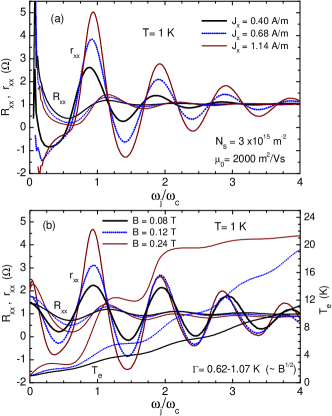
Figure 1: (Color online) (a) Resistivity $R_{xx}$ and differential resistivity $r_{xx}$ versus $\omega_{j}/\omega_{c}$ at fixed DC current density $J_{x}=0.40,0.68$ or 1.14 A/m, and (b) $R_{xx}$, $r_{xx}$ and electron temperature $T_{\rm e}$ versus $\omega_{j}/\omega_{c}$ at fixed magnetic field $B=0.08,0.12$ or 0.24 T, for a GaAs-based 2D system having electron density $N_{\rm s}=3.0\times 10^{15}$ m^-2, linear mobility $\mu_{0}=2000$ m²/Vs, $\alpha=10$ at $T=1$ K, assuming SR scattering.

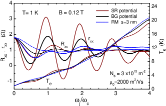
Figure 2: (Color online) $R_{xx}$, $r_{xx}$ and $T_{\rm e}$ versus $\omega_{j}/\omega_{c}$ at fixed magnetic field $B=0.12$ T for the same system as described in Fig. 1 but subject to SR, BG or RM scattering potentials.

Figure 1(a) presents the calculated resistivity $R_{xx}$ and differential resistivity $r_{xx}$ versus the inverse magnetic field $1/B$ in terms of $\omega_{j}/\omega_{c}$ at lattice temperature $T=1$ K, for a 2D system with electron density $N_{\rm s}=3.0\times 10^{15}$ m^-2 and linear mobility $\mu_{0}=2000$ m²/Vs subject to three different bias dc current densities $J_{x}=0.40,0.68$ and 1.14 A/m, which correspond to $\omega_{j}/2\pi=32.3,62.2$ and 103.6 GHz respectively. The elastic scattering is assumed to be short ranged, and the broadening parameter $\alpha=10$, i.e. $B^{1/2}$-dependent $\Gamma$, $\simeq 0.62$ K at $B=0.08$ T. Oscillations in resistivity $R_{xx}$, especially in differential resistivity $r_{xx}$ show up remarkably, having an approximate period $\Delta(\omega_{j}/\omega_{c})\sim 1$. The oscillation amplitude decays with increasing $\omega_{j}/\omega_{c}$ (reducing $B$ field, due to increasing overlap of LLs) at fixed bias current but increases with increasing bias current density within the $J_{x}$ range shown. The maxima (minima) of the differential resistivity $r_{xx}$ locate quite close to (but somewhat lower than) the integers (half integers) of $\omega_{j}/\omega_{c}$, while the maxima (minima) of the total resistivity $R_{xx}$ are shifted around a quarter period higher. These features are in good agreement with recent experimental findings.WZ0608727 Note that the electron temperature $T_{\rm e}$ (not shown) exhibits only a weak variation with changing $B$ field at each fixed dc.

In Fig. 1(b) we plot $R_{xx}$, $r_{xx}$ and electron temperature $T_{\rm e}$ versus the dc density in terms of $\omega_{j}/\omega_{c}$ at fixed magnetic fields $B=0.08,0.12$ and 0.24 T for the same system. Remarkable $R_{xx}$ and $r_{xx}$ oscillations with approximate period $\Delta(\omega_{j}/\omega_{c})\sim 1$ and maxima (minima) positions similar to those in Fig. 1(a) can be seen in this current-sweeping figure but here the oscillation decay with increasing $\omega_{j}/\omega_{c}$ is due to increase in the electron temperature. At lower $\omega_{j}/\omega_{c}$ range, the oscillation amplitude of high $B$-field case is apparently larger than low $B$-field case when the electron temperature $T_{\rm e}$ is still in the range less than or around $10$ K. However, in the case of $B=0.24$ T the oscillation amplitude decays rapidly with increasing $\omega_{j}/\omega_{c}$ due to the rapid increase of electron temperature, which rises up to $20$ K range around $\omega_{j}/\omega_{c}=2$. In comparison, the amplitude decay is much slower in the case of $B=0.08$ T because of the slow $T_{\rm e}$ rise. Furthermore, the periods of $R_{xx}$ and $r_{xx}$ oscillations are also somewhat shrunk by the rise of $T_{\rm e}$, as can be seen at higher orders in the $B=0.24$ T case.

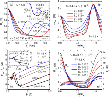
Figure 3: (Color online) Calculated $R_{xx}$, $r_{xx}$, $R_{xx}/R_{0}$, $\Delta r_{xx}=r_{xx}-R_{0}$ and $T_{\rm e}$ for a GaAs-based 2D system with $N_{\rm s}=3.0\times 10^{15}$ m^-2 at lattice temperature $T=1.5$ K subject to a mixed SR and BG elastic scattering. The LL width is taken to be $B^{1/2}$ dependent with $\Gamma=0.4$ K at $B=0.08$ T. The insects illustrate the case of fixed LL width $\Gamma=0.4$ K.

Note that though the periods of these resistance oscillations are roughly the same in terms of $\omega_{j}/\omega_{c}$, their amplitude and the detailed behavior depend strongly on the form of the scattering potential $U({\bf q}_{\|})$ in Eq. (3). To have an idea of this scattering potential effect we plot, in Fig. 2, $R_{xx}$, $r_{xx}$, and $T_{\rm e}$ as functions of $\omega_{j}/\omega_{c}$ at a fixed magnetic field $B=0.12$ T for the same 2D system but with the dominant elastic scatterings, respectively, due to short-range (SR) disorder, charged impurities in the background (BG), or ionized impurities locating a distance $s=3$ nm away from the 2D sheet (RM).Lei851 $R_{xx}$ and $r_{xx}$ exhibit the strongest oscillations in the case of SR potential, with a feature that the second minimum of $r_{xx}$ goes deeper into negative direction than the first minimum. In the case of BG scattering $R_{xx}$ and $r_{xx}$ oscillations, though weaker than those of SR-scattering case, still appear quite substantial and the first minimum of $r_{xx}$ turns out to be the deepest one of all minima. In the case of RM ($s=3$ nm) scattering, these current-induced resistance oscillations, though existing, become much weaker than those of SR and BG scatterings.

Fig. 3 presents the calculated $R_{xx}$, $r_{xx}$, $R_{xx}/R_{0}$, $\Delta r_{xx}=r_{xx}-R_{0}$ ($R_{0}$ is the resistivity at zero dc bias) and $T_{\rm e}$, for another GaAs-based 2D system with $N_{\rm s}=3.0\times 10^{15}$ m^-2, $\mu_{0}=1500$ m²/Vs at $T=1.5$ K, focusing on the first oscillation period of $\omega_{j}/\omega_{c}$. The elastic scatterings are assumed due to a mixture of SR and BG impurities (with 2:1 contribution ratio to the linear mobility).Lei851 The broadening parameter is taken to be $\alpha=3$ ($B^{1/2}$-dependent $\Gamma$, $\simeq 0.4$ K at $B=0.08$ T), a somewhat smaller LL width to keep the system mainly in the separated LL regime. The insets of Figs. 3a and 3c show the results using a $B$-independent $\Gamma=0.4$ K. All the main features found in the experiment in the case of separated Landau levels,WZ0608727 e.g., the dramatic initial suppression of the magnetoresistivity with increasing dc density, the widening and deepening of the first minimum range with increasing $B$ field, a few resolvable oscillations of $r_{xx}$ at lower $B$, dramatic reduction of it at higher magnetic field, etc., are well reproduced. Note that the width of the half zero-bias peak in terms of $\omega_{j}$ accurately reflects the width of LLs, as can be seen clearly in Fig. 3(a) and its inset. This suggests an ideal way to determine the width of LLs.

This work was supported by the projects of National Science Foundation of China and Shanghai Municipal Commission of Science and Technology.

References

- (1) V. I. Ryzhii, Sov. Phys. Solid State 11, 2087 (1970).
- (2) M. A. Zudov, R. R. Du, J. A. Simmons, and J. L. Reno, Phys. Rev. B 64, 201311(R) (2001).
- (3) P. D. Ye, L. W. Engel, D. C. Tsui, J. A. Simmons, J. R. Wendt, G. A. Vawter, and J. L. Reno, Appl. Phys. Lett. 79, 2193 (2001).
- (4) R. G. Mani, J. H. Smet, K. von Klitzing, V. Narayanamurti, W. B. Johnson, and V. Umansky, Nature (London) 420, 646 (2002).
- (5) M. A. Zudov, R. R. Du, L. N. Pfeiffer, and K. W. West, Phys. Rev. Lett. 90, 046807 (2003).
- (6) S. I. Dorozhkin, JETP Lett. 77, 577 (2003).
- (7) A. C. Durst, S. Sachdev, N. Read, and S. M. Girvin, Phys. Rev. Lett. 91, 086803 (2003).
- (8) X. .L. Lei and S. Y. Liu, Phys. Rev. Lett. 91, 226805 (2003); X. L. Lei, J. Phys.: Condens. Matter 16, 4045 (2004).
- (9) Tai-Kai Ng and Lixin Dai, Phys. Rev. B 72, 235333 (2005).
- (10) C. L. Yang, J. Zhang, R. R. Du, J. A. Simmons, and J. L. Reno, Phys. Rev. Lett. 89, 076801 (2002).
- (11) A. A. Bykov, J. Q. Zhang, S. Vitkalov, A. K. Kalagin, and A. K. Bakarov, Phys. Rev. B 72, 245307 (2005).
- (12) J. Q. Zhang, S. Vitkalov, A. A. Bykov, A. K. Kalagin, and A. K. Bakarov, Phys. Rev. B 75, 081305 (R), (2007).
- (13) W. Zhang, H. -S. Chiang, M. A. Zudov, L. N. Pfeiffer, and K. W. West, Phys. Rev. B 75, 041304(R) (2007).
- (14) C. S. Ting, S. C. Ying, and J. J. Quinn, Phys. Rev. B 14, 4439 (1976); Phys. Rev. B 16, 5394 (1977).
- (15) X. L. Lei and C. S. Ting, Phys. Rev. B 30, 4809 (1984); Phys. Rev. B 32, 1112 (1985).
- (16) X. L. Lei, J. L. Birman, and C. S. Ting, J. Appl. Phys. 58, 2270 (1985).
- (17) W. Cai, X. L. Lei, and C. S. Ting, Phys. Rev. B 31, 4070 (1985); X. L. Lei, W. Cai, and C. S. Ting, J. Phys. C, 18, 4315 (1985).
- (18) T. Ando, A. B. Fowler, and F. Stern, Rev. Mod. Phys. 54, 437 (1982).