Master equation approach to DNA-breathing in heteropolymer DNA

Tobias Ambjörnsson ambjorn@nordita.dk NORDITA (Nordic Institute for Theoretical Physics), Blegdamsvej 17, DK-2100 Copenhagen Ø, Denmark. Present address: Department of Chemistry, Massachusetts Institute of Technology, 77 Massachusetts Avenue, Cambridge, MA 02139, USA    Suman K. Banik Dept. of Physics, Virginia Polytechnic Institute and State University, Blacksburg, VA 24061-0435, USA    Michael A. Lomholt NORDITA (Nordic Institute for Theoretical Physics), Blegdamsvej 17, DK-2100 Copenhagen Ø, Denmark. Present address: Department of Physics, University of Ottawa, 150 Louis Pasteur, Ottawa, Ontario K1N 6N5, Canada    Ralf Metzler metz@nordita.dk NORDITA (Nordic Institute for Theoretical Physics), Blegdamsvej 17, DK-2100 Copenhagen Ø, Denmark. Present address: Department of Physics, University of Ottawa, 150 Louis Pasteur, Ottawa, Ontario K1N 6N5, Canada
Abstract

After crossing an initial barrier to break the first base-pair (bp) in double-stranded DNA, the disruption of further bps is characterized by free energies between less than one to a few kBTsubscript𝑘𝐵𝑇k_{B}T. This causes the opening of intermittent single-stranded bubbles. Their unzipping and zipping dynamics can be monitored by single molecule fluorescence or NMR methods. We here establish a dynamic description of this DNA-breathing in a heteropolymer DNA in terms of a master equation that governs the time evolution of the joint probability distribution for the bubble size and position along the sequence. The transfer coefficients are based on the Poland-Scheraga free energy model. We derive the autocorrelation function for the bubble dynamics and the associated relaxation time spectrum. In particular, we show how one can obtain the probability densities of individual bubble lifetimes and of the waiting times between successive bubble events from the master equation. A comparison to results of a stochastic Gillespie simulation shows excellent agreement.

pacs:
05.40.-a,82.37.-j,87.15.-v,02.50.-r

I Introduction

Even at room temperature the DNA double-helix opens up locally to form intermittent flexible single-stranded domains, the DNA-bubbles. Their size increases from a few broken base-pairs (bps) to a few hundred open bps just below the melting temperature Tmsubscript𝑇𝑚T_{m}, until a transition occurs to full denaturation kornberg ; poland ; wartell ; cantor_schimmel . DNA stability is effected by combination of the free energies ϵhbsubscriptitalic-ϵhb\epsilon_{\rm hb} for breaking a Watson-Crick hydrogen bond between complementary AT and GC bases in a single bp, and the ten independent stacking free energies ϵstsubscriptitalic-ϵst\epsilon_{\rm st} for disrupting the interactions between a nearest neighbor pair of bps. At 100 mM NaCl concentration and T=37𝑇superscript37T=37^{\circ}C the hydrogen bonding amounts to ϵhb=1.0kBTsubscriptitalic-ϵhb1.0subscript𝑘𝐵𝑇\epsilon_{\rm hb}=1.0k_{B}T for a single AT and 0.2kBT0.2subscript𝑘𝐵𝑇0.2k_{B}T for a GC-bond REM . The weakest (strongest) stacking energies was found to be the TA/AT (GC/CG) with free energies ϵst=0.9kBTsubscriptitalic-ϵst0.9subscript𝑘𝐵𝑇\epsilon_{\rm st}=-0.9k_{B}T (4.1kBT4.1subscript𝑘𝐵𝑇-4.1k_{B}T). Note that negative values for the free energies denote stable states. The relatively small free energies for base stacking stem from the fact that relatively large amounts of binding enthalpy on the one hand, and entropy release on breaking the stacking interactions and Watson-Crick bonds on the other hand, almost cancel. Bubble initiation, in contrast, is characterized by breaking of two stacking interactions with the first bp, whose enthalpy cost cannot be balanced by the two, still strongly confined, liberated bases. Thus, the creation of two boundaries between the intact double-helix and the bubble nucleus is associated with an activation cost of some 7 to 12 kBTsubscript𝑘𝐵𝑇k_{B}T corresponding to the Boltzmann factor σ0103105similar-to-or-equalssubscript𝜎0superscript103superscript105\sigma_{0}\simeq 10^{-3}\ldots 10^{-5} poland ; wartell ; blake ; blossey . The cooperativity parameter σ0subscript𝜎0\sigma_{0} is related to the ring-factor ξ𝜉\xi used in FK ; FK1 , see below. The high bubble initiation barrier indeed guarantees the stability of DNA at physiological conditions. Bubble opening occurs predominantly in zones rich in the weaker AT bps; with increasing T𝑇T, they spread to regions with progressively higher GC content wartell ; poland ; kornberg . Thermally driven, a DNA-bubble fluctuates in size by relative random motion of the two zipper forks. In addition to observations using NMR techniques gueron , this DNA-breathing was recently monitored on the single bubble level by fluorescence correlation methods, demonstrating a multistate kinetics that reflects the stepwise unzipping and zipping of bps. The lifetime of a bubble was shown to range up to a few ms altan .

From a biology or biochemistry point of view, DNA-breathing is of interest, as it is implicated to influence the binding of binding proteins, enzymes, and other chemicals to DNA. Thus, the relatively fast bubble dynamics with respect to the binding rates of proteins, that selectively bind to single-stranded DNA, provides a kinetic block preventing DNA denaturation through these proteins rich1 ; pant ; pant1 . This was investigated in detail on the bases of a homopolymer approach in Refs. tobias ; JPC . Similarly, the increase of the bubble formation probability as well as of the bubble lifetime at certain places along the sequence is believed to facilitate the initiation of transcription by RNA polymerase. This latter point is studied in depth in Ref. bj .

In this paper we investigate a (2+1)21(2+1)-variable master equation, that governs the time evolution of the probability distribution P(m,xL,t)𝑃𝑚subscript𝑥𝐿𝑡P(m,x_{L},t) to find a bubble consisting of m𝑚m broken bps with left fork position xLsubscript𝑥𝐿x_{L} along the sequence. With this approach, that is, an arbitrary DNA sequence can be analyzed, and its breathing behavior predicted. We discuss the exact form of the transfer matrix containing the rate coefficients for all permitted moves, and derive the bubble autocorrelation function with associated relaxation time spectrum. To be able to connect to the time series obtained from the complementary stochastic simulation, we derive the probability densities according to which individual bubble lifetimes and the time intervals between successive bubble events are distributed. Finally, we show that in the homopolymer limit, analytical results can be obtained.

II One bubble partition function and transfer coefficients
Refer to caption
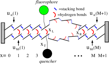
Figure 1: Clamped DNA domain with internal bps x=1𝑥1x=1 to M𝑀M, statistical weights uhb(x)subscript𝑢hb𝑥u_{\rm hb}(x), ust(x)subscript𝑢st𝑥u_{\rm st}(x), and tag position xTsubscript𝑥𝑇x_{T}. The DNA sequence enters through the statistical weights ust(x)subscript𝑢st𝑥u_{\rm st}(x) and uhb(x)subscript𝑢hb𝑥u_{\rm hb}(x) for disrupting stacking and hydrogen bonds, respectively. The bubble breathing process consists of the initiation of a bubble and the subsequent motion of the forks at positions xLsubscript𝑥𝐿x_{L} and xRsubscript𝑥𝑅x_{R}, see also Fig. 2.

Below the melting temperature Tmsubscript𝑇𝑚T_{m}, a single bubble can be considered to be statistically independent due to the high nucleation barrier for initiating a bubble quantified by σ01much-less-thansubscript𝜎01\sigma_{0}\ll 1 JPC , such that opening and merging of multiple bubbles are rare, and a one-bubble picture is appropriate. In the particular case of the bubble constructs used in the fluorescence correlation experiments of Ref. altan , the sequence is designed such that there is a single bubble domain. Referring to these constructs, we consider a segment of double-stranded DNA with M𝑀M internal bps. These bps are clamped at both ends such that the bps x=0𝑥0x=0 and x=M+1𝑥𝑀1x=M+1 are always closed (Fig. 1). The sequence of bps determines the Boltzmann weights uhb(x)=exp{ϵhb(x)/(kBT)}subscript𝑢hb𝑥subscriptitalic-ϵhb𝑥subscript𝑘𝐵𝑇u_{\rm hb}(x)=\exp\{\epsilon_{\rm hb}(x)/(k_{B}T)\} for Watson-Crick hydrogen bonding at position x𝑥x, and the Boltzmann factor ust(x)=exp{ϵst(x)/(kBT)}subscript𝑢st𝑥subscriptitalic-ϵst𝑥subscript𝑘𝐵𝑇u_{\rm st}(x)=\exp\{\epsilon_{\rm st}(x)/(k_{B}T)\} for pure bp-bp stacking between bps x1𝑥1x-1 and x𝑥x, respectively. In the bubble domain, the left and right zipper fork positions xLsubscript𝑥𝐿x_{L} and xRsubscript𝑥𝑅x_{R} denoting the right- and leftmost closed bp of the bubble are stochastic quantities, whose random motion underlies the bubble dynamics.

Instead of using the fork positions xLsubscript𝑥𝐿x_{L} and xRsubscript𝑥𝑅x_{R}, we prefer to work with the left fork position xLsubscript𝑥𝐿x_{L} and the bubble size m=xRxL1𝑚subscript𝑥𝑅subscript𝑥𝐿1m=x_{R}-x_{L}-1. For these variables, the partition function of the bubble becomes

𝒵(xL,m)=ξ(1+m)cx=xL+1xL+muhb(x)x=xL+1xL+m+1ust(x)𝒵subscript𝑥𝐿𝑚superscript𝜉superscript1𝑚𝑐superscriptsubscriptproduct𝑥subscript𝑥𝐿1subscript𝑥𝐿𝑚subscript𝑢hb𝑥superscriptsubscriptproduct𝑥subscript𝑥𝐿1subscript𝑥𝐿𝑚1subscript𝑢st𝑥\mathscr{Z}(x_{L},m)=\frac{\xi^{\prime}}{(1+m)^{c}}\prod_{x=x_{L}+1}^{x_{L}+m}u_{\rm hb}(x)\prod_{x=x_{L}+1}^{x_{L}+m+1}u_{\rm st}(x) (1)

for m1𝑚1m\geq 1. At m=0𝑚0m=0, we define 𝒵(m=0)=1𝒵𝑚01\mathscr{Z}(m=0)=1. In relation (1), instead of the usual cooperativity parameter σ0subscript𝜎0\sigma_{0} we use the factor ξ=2cξsuperscript𝜉superscript2𝑐𝜉\xi^{\prime}=2^{c}\xi related to the ring factor ξ103𝜉superscript103\xi\approx 10^{-3} introduced in Ref. FK . For a homopolymer, this ξ𝜉\xi is related to σ0subscript𝜎0\sigma_{0} by σ0=ξexp{ϵst/(kBT)}subscript𝜎0𝜉subscriptitalic-ϵstsubscript𝑘𝐵𝑇\sigma_{0}=\xi\exp\{\epsilon_{\mathrm{st}}/(k_{B}T)\} FK . The denominator in Eq. (1) represents the entropy loss on formation of a closed polymer loop, where the offset by one accounts for finite size effects blake ; fixman . The associated critical exponent is c=1.76𝑐1.76c=1.76 richard . For a given bubble size, the partition (1) counts m𝑚m contributions from broken hydrogen bonds and m+1𝑚1m+1 from disrupted stacking interactions. The partition (1) defines the equilibrium probability

Peq(xL,m)=𝒵(xL,m)𝒵(0)+m=1MxL=0Mm𝒵(xL,m)superscript𝑃eqsubscript𝑥𝐿𝑚𝒵subscript𝑥𝐿𝑚𝒵0superscriptsubscript𝑚1𝑀superscriptsubscriptsubscript𝑥𝐿0𝑀𝑚𝒵subscript𝑥𝐿𝑚P^{\rm eq}(x_{L},m)=\frac{\mathscr{Z}(x_{L},m)}{\mathscr{Z}(0)+\sum_{m=1}^{M}\sum_{x_{L}=0}^{M-m}\mathscr{Z}(x_{L},m)} (2)

for finding a bubble of size m𝑚m at location xLsubscript𝑥𝐿x_{L}.

The two variables m𝑚m and xLsubscript𝑥𝐿x_{L} are the slow variables of the breathing dynamics, while the polymeric degrees of freedom of the relatively small bubble enter effectively through the partition (1). We moreover assume that the bubble is always close to thermal equilibrium such that the partition (1) defines the transition probabilities between different states. These conditions allow us to introduce the master equation (9) with its transfer matrix 𝒲𝒲\mathscr{W} below. To introduce the underlying time scales, we first define the transfer coefficients.
Refer to caption
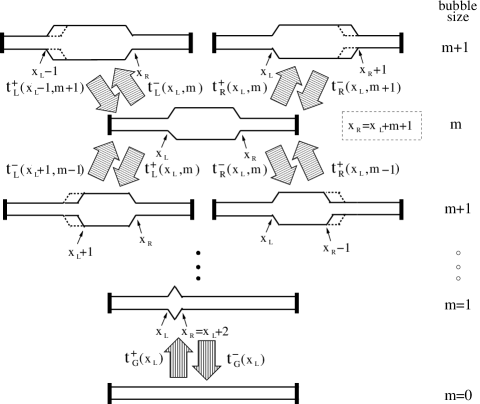
Figure 2: Possible bubble (un)zipping transitions: for m2𝑚2m\geq 2, the four transfer rates 𝗍L/R±(xL,m)subscriptsuperscript𝗍plus-or-minus𝐿𝑅subscript𝑥𝐿𝑚\mathsf{t}^{\pm}_{L/R}(x_{L},m) completely determine the transitions out of this state; the coefficients 𝗍L±(xL1,m±1)superscriptsubscript𝗍𝐿plus-or-minusminus-or-plussubscript𝑥𝐿1plus-or-minus𝑚1\mathsf{t}_{L}^{\pm}(x_{L}\mp 1,m\pm 1) and 𝗍R±(xL,m1)superscriptsubscript𝗍𝑅plus-or-minussubscript𝑥𝐿minus-or-plus𝑚1\mathsf{t}_{R}^{\pm}(x_{L},m\mp 1) specify the possible jumps into this state. Jumps between state m=1𝑚1m=1 and ground state m=0𝑚0m=0 are described by 𝗍G+(xL)subscriptsuperscript𝗍𝐺subscript𝑥𝐿\mathsf{t}^{+}_{G}(x_{L}) and 𝗍G(xL)subscriptsuperscript𝗍𝐺subscript𝑥𝐿\mathsf{t}^{-}_{G}(x_{L}).

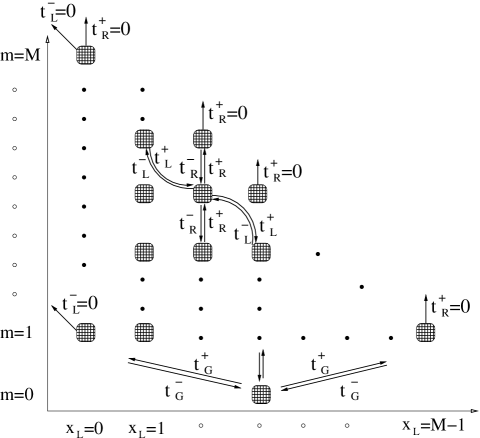
The allowed transitions with the associated transfer (rate) coefficients are sketched in Fig. 2. The left zipper fork is characterized by the rate 𝗍L+(xL,m)subscriptsuperscript𝗍𝐿subscript𝑥𝐿𝑚\mathsf{t}^{+}_{L}(x_{L},m) corresponding to the process xLxL+1subscript𝑥𝐿subscript𝑥𝐿1x_{L}\rightarrow x_{L}+1 of bubble size decrease, and 𝗍L(xL,m)subscriptsuperscript𝗍𝐿subscript𝑥𝐿𝑚\mathsf{t}^{-}_{L}(x_{L},m) for xLxL1subscript𝑥𝐿subscript𝑥𝐿1x_{L}\rightarrow x_{L}-1 (bubble size increase). Similarly, we introduce 𝗍R+(xL,m)subscriptsuperscript𝗍𝑅subscript𝑥𝐿𝑚\mathsf{t}^{+}_{R}(x_{L},m) for xRxR+1subscript𝑥𝑅subscript𝑥𝑅1x_{R}\rightarrow x_{R}+1 (bubble size increase) and 𝗍R(xL,m)subscriptsuperscript𝗍𝑅subscript𝑥𝐿𝑚\mathsf{t}^{-}_{R}(x_{L},m) for xRxR1subscript𝑥𝑅subscript𝑥𝑅1x_{R}\rightarrow x_{R}-1 (decrease). These rates are valid for transitions between states with m1𝑚1m\geq 1. Bubble opening (initiation) m=0m=1𝑚0𝑚1m=0\rightarrow m=1 is quantified by 𝗍G+(xL)superscriptsubscript𝗍𝐺subscript𝑥𝐿\mathsf{t}_{G}^{+}(x_{L}), and bubble closing (annihilation) m=10𝑚10m=1\to 0 by 𝗍G(xL)superscriptsubscript𝗍𝐺subscript𝑥𝐿\mathsf{t}_{G}^{-}(x_{L}). Note that by our definitions 𝗍G+(xL)superscriptsubscript𝗍𝐺subscript𝑥𝐿\mathsf{t}_{G}^{+}(x_{L}) and 𝗍G(xL)superscriptsubscript𝗍𝐺subscript𝑥𝐿\mathsf{t}_{G}^{-}(x_{L}) actually correspond to bubble opening/closing at x=xL+1𝑥subscript𝑥𝐿1x=x_{L}+1. Clamping requires that xL0subscript𝑥𝐿0x_{L}\geq 0 and xRM+1subscript𝑥𝑅𝑀1x_{R}\leq M+1, corresponding to reflecting boundary conditions REM0

𝗍L(xL=0,m)=𝗍R+(xL,m=MxL)=0.superscriptsubscript𝗍𝐿subscript𝑥𝐿0𝑚superscriptsubscript𝗍𝑅subscript𝑥𝐿𝑚𝑀subscript𝑥𝐿0\mathsf{t}_{L}^{-}(x_{L}=0,m)=\mathsf{t}_{R}^{+}(x_{L},m=M-x_{L})=0. (3)

In Fig. 3 we sketch schematically the allowed transitions in the m𝑚m-xLsubscript𝑥𝐿x_{L} plane.

In order to define the various transfer rates 𝗍𝗍\mathsf{t}, we firstly impose the detailed balance conditions (compare Risken ; van_Kampen )

𝗍L+(xL1,m+1)𝗍L(xL,m)superscriptsubscript𝗍𝐿subscript𝑥𝐿1𝑚1superscriptsubscript𝗍𝐿subscript𝑥𝐿𝑚\displaystyle\frac{\mathsf{t}_{L}^{+}(x_{L}-1,m+1)}{\mathsf{t}_{L}^{-}(x_{L},m)} =\displaystyle= Peq(xL,m)Peq(xL1,m+1)subscript𝑃eqsubscript𝑥𝐿𝑚subscript𝑃eqsubscript𝑥𝐿1𝑚1\displaystyle\frac{P_{\rm eq}(x_{L},m)}{P_{\rm eq}(x_{L}-1,m+1)} (4a)
𝗍R(xL,m+1)𝗍R+(xL,m)superscriptsubscript𝗍𝑅subscript𝑥𝐿𝑚1superscriptsubscript𝗍𝑅subscript𝑥𝐿𝑚\displaystyle\frac{\mathsf{t}_{R}^{-}(x_{L},m+1)}{\mathsf{t}_{R}^{+}(x_{L},m)} =\displaystyle= Peq(xL,m)Peq(xL,m+1)subscript𝑃eqsubscript𝑥𝐿𝑚subscript𝑃eqsubscript𝑥𝐿𝑚1\displaystyle\frac{P_{\rm eq}(x_{L},m)}{P_{\rm eq}(x_{L},m+1)} (4b)
𝗍G+(xL)𝗍G(xL)superscriptsubscript𝗍𝐺subscript𝑥𝐿superscriptsubscript𝗍𝐺subscript𝑥𝐿\displaystyle\frac{\mathsf{t}_{G}^{+}(x_{L})}{\mathsf{t}_{G}^{-}(x_{L})} =\displaystyle= Peq(xL,1)Peq(0),subscript𝑃eqsubscript𝑥𝐿1subscript𝑃eq0\displaystyle\frac{P_{\rm eq}(x_{L},1)}{P_{\rm eq}(0)}, (4c)

that ensure relaxation toward the equilibrium distribution Peq(xL,m)superscript𝑃eqsubscript𝑥𝐿𝑚P^{\rm eq}(x_{L},m), see Eq. (2). The latter can be seen by recalling that the equilibrium distribution (2) is based on the Boltzmann factors uhbsubscript𝑢hbu_{\mathrm{hb}} and ustsubscript𝑢stu_{\mathrm{st}} through the partition (1). The detailed balance conditions do not uniquely define the transfer rates 𝗍𝗍\mathsf{t}, leaving a certain freedom of choice van_Kampen . We use the following conventions.
Refer to caption
Figure 3: Schematic representation of the (xL,m)subscript𝑥𝐿𝑚(x_{L},m)-lattice on which the DNA-bubble jump process takes place, with the permitted transitions; compare to Figs. 1 and 2. The boundary conditions Eq. (3) are also indicated.

To define the zipping rate, we assume that it is independent of the position x𝑥x along the DNA sequence. The picture behind is that the closure of the bp is dominated by the requirement that the two bases diffuse in real space until mutual encounter and eventual bond formation. As sterically AT and GC bps are very similar, the zipping rate should not significantly vary with the individual nature of the involved bps, and we choose the constant rate k/2𝑘2k/2, see below. This rate k𝑘k is the only adjustable parameter of our model, and has to be independently determined from experiment or more fundamental models. This choice, as mentioned above, is not unique. Instead, an x𝑥x-dependence of k𝑘k could easily be introduced by choosing different powers of the statistical weights entering the rate coefficients such that they still fulfill detailed balance.

Decrease in bubble size due to zipping close of the bp closest to either the left or the right zipper fork is therefore ruled by

𝗍L+(xL,m)|m2=tR(xL,m)|m2=k2,evaluated-atsubscriptsuperscript𝗍𝐿subscript𝑥𝐿𝑚𝑚2evaluated-atsubscriptsuperscript𝑡𝑅subscript𝑥𝐿𝑚𝑚2𝑘2\mathsf{t}^{+}_{L}(x_{L},m)|_{m\geq 2}=t^{-}_{R}(x_{L},m)|_{m\geq 2}=\frac{k}{2}, (5)

respectively. The factor 1/2121/2 is introduced for consistency with previous approaches tobias ; JPC . Note that for simplicity we do not introduce the hook exponent discussed in previous studies PRL ; JPC ; bj . This exponent should be important for large bubbles, when during the zipping process not only the bp at the zipper fork is moved, but also part of the vicinal single-strand is dragged or pushed along Di_Marzio_Guttman_Hoffman ; PRL ; JPC .

Increase in bubble size is controlled by

𝗍L(xL,m)superscriptsubscript𝗍𝐿subscript𝑥𝐿𝑚\displaystyle\mathsf{t}_{L}^{-}(x_{L},m) =\displaystyle= k2ust(xL)uhb(xL)s(m),𝑘2subscript𝑢stsubscript𝑥𝐿subscript𝑢hbsubscript𝑥𝐿𝑠𝑚\displaystyle\frac{k}{2}u_{\rm st}(x_{L})u_{\rm hb}(x_{L})s(m), (6a)
𝗍R+(xL,m)superscriptsubscript𝗍𝑅subscript𝑥𝐿𝑚\displaystyle\mathsf{t}_{R}^{+}(x_{L},m) =\displaystyle= k2ust(xR+1)uhb(xR)s(m),𝑘2subscript𝑢stsubscript𝑥𝑅1subscript𝑢hbsubscript𝑥𝑅𝑠𝑚\displaystyle\frac{k}{2}u_{\rm st}(x_{R}+1)u_{\rm hb}(x_{R})s(m), (6b)

for m1𝑚1m\geq 1, where

s(m)=(1+m2+m)c.𝑠𝑚superscript1𝑚2𝑚𝑐s(m)=\left(\frac{1+m}{2+m}\right)^{c}. (7)

For m1𝑚1m\geq 1 we thus take the bubble increase rate coefficients proportional to the first power of the Arrhenius factor ustuhb=exp{(ϵhb+ϵst)/[kBT]}subscript𝑢stsubscript𝑢hbsubscriptitalic-ϵhbsubscriptitalic-ϵstdelimited-[]subscript𝑘𝐵𝑇u_{\rm st}u_{\rm hb}=\exp\{(\epsilon_{\mathrm{hb}}+\epsilon_{\mathrm{st}})/[k_{B}T]\} times the loop correction s(m)𝑠𝑚s(m). We stress that Eqs. (6a) and (6b) are dictated by the detailed balance condition, once the convention (5) is established. As noted, detailed balance would still be fulfilled, for instance, if only a fractional power αqsuperscript𝛼𝑞\alpha^{q} of the Arrhenius factor α𝛼\alpha appeared in the opening rates if complemented by the respective power α1qsuperscript𝛼1𝑞\alpha^{1-q} in the closing rates.

Finally, we define

𝗍G+(xL)superscriptsubscript𝗍𝐺subscript𝑥𝐿\displaystyle\mathsf{t}_{G}^{+}(x_{L}) =\displaystyle= kξs(0)ust(xL+1)uhb(xL+1)𝑘superscript𝜉𝑠0subscript𝑢stsubscript𝑥𝐿1subscript𝑢hbsubscript𝑥𝐿1\displaystyle k\xi^{\prime}s(0)u_{\rm st}(x_{L}+1)u_{\rm hb}(x_{L}+1)
×ust(xL+2)absentsubscript𝑢stsubscript𝑥𝐿2\displaystyle\times u_{\rm st}(x_{L}+2)
𝗍G(xL)superscriptsubscript𝗍𝐺subscript𝑥𝐿\displaystyle\mathsf{t}_{G}^{-}(x_{L}) =\displaystyle= k𝑘\displaystyle k (8b)

for bubble initiation and annihilation from and to the zero-bubble state m=0𝑚0m=0, with the bubble initiation factor ξsuperscript𝜉\xi^{\prime} in the expression for 𝗍G+superscriptsubscript𝗍𝐺\mathsf{t}_{G}^{+}. As bubble initiation involves breaking of two stacking interactions at consecutive bps, we have the factor ust(xL+1)ust(xL+2)subscript𝑢stsubscript𝑥𝐿1subscript𝑢stsubscript𝑥𝐿2u_{\rm st}(x_{L}+1)u_{\rm st}(x_{L}+2) in expression (8). The last open bp can zip close from either side, so the bubble closing rate 𝗍G(xL)superscriptsubscript𝗍𝐺subscript𝑥𝐿\mathsf{t}_{G}^{-}(x_{L}) makes up twice the zipping rate of a single fork.

The rates 𝗍𝗍\mathsf{t} together with the boundary conditions fully determine the bubble dynamics. In the next Section, we establish the master equation for the time evolution of the distribution P(m,xL,t)𝑃𝑚subscript𝑥𝐿𝑡P(m,x_{L},t) and derive the associated quantities.

III Master equation for DNA-breathing

The joint probability distribution P(t)=P(xL,m,t;xL,m,0)𝑃𝑡𝑃subscript𝑥𝐿𝑚𝑡superscriptsubscript𝑥𝐿superscript𝑚0P(t)=P(x_{L},m,t;x_{L}^{\prime},m^{\prime},0) measures the likelihood that at time t𝑡t the system is in state {xL,m}subscript𝑥𝐿𝑚\{x_{L},m\} and that at t=0𝑡0t=0 it was in state {xL,m}superscriptsubscript𝑥𝐿superscript𝑚\{x_{L}^{\prime},m^{\prime}\}. Its time evolution is controlled by the master equation

tP(t)=𝒲P(t).𝑡𝑃𝑡𝒲𝑃𝑡\frac{\partial}{\partial t}P(t)=\mathscr{W}P(t). (9)

The explicit form of the transfer matrix 𝒲𝒲\mathscr{W} is discussed in detail in Sec. IV. Here, we concentrate on how to derive the quantities relevant for the description of DNA-breathing experiments. In that course we introduce the eigenmode ansatz van_Kampen ; Risken

P(t)=pcpQpexp(ηpt),𝑃𝑡subscript𝑝subscript𝑐𝑝subscript𝑄𝑝subscript𝜂𝑝𝑡P(t)=\sum_{p}c_{p}Q_{p}\exp(-\eta_{p}t), (10)

where the coefficients cpsubscript𝑐𝑝c_{p} are fixed by the initial condition. Combining Eqs. (10) and (9), the eigenvalue equation

𝒲Qp=ηpQp𝒲subscript𝑄𝑝subscript𝜂𝑝subscript𝑄𝑝\mathscr{W}Q_{p}=-\eta_{p}Q_{p} (11)

yields, compare Ref. van_Kampen and below for more details. The eigenvalues ηpsubscript𝜂𝑝\eta_{p} and eigenvectors Qpsubscript𝑄𝑝Q_{p} allow one to compute any quantity of interest. In fact, the autocorrelation function for bubble breathing and the corresponding relaxation time distribution are quite straightforward to obtain, see section III.1. Below, in section III.2, we discuss the more subtle point how the probability densities for the bubble lifetime and the interbubble event waiting time can be derived.

III.1 Blinking autocorrelation function of a tagged bp

Motivated by the fluorescence correlation setup in Ref. altan we are interested in the state of a tagged bp at x=xT𝑥subscript𝑥𝑇x=x_{T}, see Fig. 1. In the experiment fluorescence occurs if the bps in a ΔΔ\Delta-neighborhood of the fluorophore position xTsubscript𝑥𝑇x_{T} are open altan . Measured fluorescence blinking time series thus correspond to the stochastic variable I(t)𝐼𝑡I(t), defined by

I(t)={1at least all bps in [xTΔ,xT+Δ] open0otherwise,.𝐼𝑡cases1at least all bps in [xTΔ,xT+Δ] open0otherwiseI(t)=\left\{\begin{array}[]{cc}1&\text{at least all bps in $[x_{T}-\Delta,x_{T}+\Delta]$ open}\\ 0&\text{otherwise},\\ \end{array}\right.. (12)

The stochastic variable is I=1𝐼1I=1 if the system is in the phase space region defined by

1:{0xLxTΔ1,xTxL+ΔmMxL}.\mathbb{R}1:\{0\leqslant x_{L}\leqslant x_{T}-\Delta-1,\ x_{T}-x_{L}+\Delta\leqslant m\leqslant M-x_{L}\}. (13)

Conversely, I=0𝐼0I=0 corresponds to the complement 00\mathbb{R}0.

The equilibrium autocorrelation function of fluorescence blinking is defined by

A(xT,t)=I(t)I(0)(I)2,𝐴subscript𝑥𝑇𝑡delimited-⟨⟩𝐼𝑡𝐼0superscriptdelimited-⟨⟩𝐼2A(x_{T},t)=\langle I(t)I(0)\rangle-(\langle I\rangle)^{2}, (14)

where the angles delimited-⟨⟩\langle\cdot\rangle denote an ensemble average over the equilibrium distribution Peqsubscript𝑃eqP_{\mathrm{eq}}. A(xT,t)𝐴subscript𝑥𝑇𝑡A(x_{T},t) quantifies the relaxation dynamics of the tagged bp. This is evident from the identity

I(t)I(0)=I=01I=01Iρ(I,t;I,0)I=ρ(1,t;1,0),delimited-⟨⟩𝐼𝑡𝐼0superscriptsubscript𝐼01superscriptsubscriptsuperscript𝐼01𝐼𝜌𝐼𝑡superscript𝐼0superscript𝐼𝜌1𝑡10\langle I(t)I(0)\rangle=\sum_{I=0}^{1}\sum_{I^{\prime}=0}^{1}I\rho(I,t;I^{\prime},0)I^{\prime}=\rho(1,t;1,0), (15)

where ρ(1,t;1,0)𝜌1𝑡10\rho(1,t;1,0) is the survival probability that I(t)=1𝐼𝑡1I(t)=1 and that I(0)=1𝐼01I(0)=1. From the definition of the two regions 11\mathbb{R}1 and 00\mathbb{R}0 it follows that ρ(1,t;1,0)𝜌1𝑡10\rho(1,t;1,0) yields from summation of P(xL,m,t;xL,m,0)𝑃subscript𝑥𝐿𝑚𝑡superscriptsubscript𝑥𝐿superscript𝑚0P(x_{L},m,t;x_{L}^{\prime},m^{\prime},0) solely over region 11\mathbb{R}1:

ρ(1,t;1,0)=xL,m,xL,m1P(xL,m,t;xL,m,0).𝜌1𝑡10subscriptsubscript𝑥𝐿𝑚superscriptsubscript𝑥𝐿superscript𝑚1𝑃subscript𝑥𝐿𝑚𝑡superscriptsubscript𝑥𝐿superscript𝑚0\rho(1,t;1,0)=\sum_{x_{L},m,x_{L}^{\prime},m^{\prime}\in\mathbb{R}1}P(x_{L},m,t;x_{L}^{\prime},m^{\prime},0). (16)

Together with Eq. (15), combined with the eigenmode decomposition (10), and under the assumption that initially the system is at equilibrium, we obtain

P(xL,m,0;xL,m,0)=δmmδxLxLPeq(xL,m),𝑃subscript𝑥𝐿𝑚0superscriptsubscript𝑥𝐿superscript𝑚0subscript𝛿𝑚superscript𝑚subscript𝛿subscript𝑥𝐿superscriptsubscript𝑥𝐿subscript𝑃eqsubscript𝑥𝐿𝑚P(x_{L},m,0;x_{L}^{\prime},m^{\prime},0)=\delta_{mm^{\prime}}\delta_{x_{L}x_{L}^{\prime}}P_{\rm eq}(x_{L},m), (17)

such that we can rewrite the autocorrelation function (14) in the form

A(xT,t)=p0[Tp(xT)]2exp(t/τp).𝐴subscript𝑥𝑇𝑡subscript𝑝0superscriptdelimited-[]subscript𝑇𝑝subscript𝑥𝑇2𝑡subscript𝜏𝑝A(x_{T},t)=\sum_{p\neq 0}\left[T_{p}(x_{T})\right]^{2}\exp(-t/\tau_{p}). (18)

Here, we use the relaxation times τp=1/ηpsubscript𝜏𝑝1subscript𝜂𝑝\tau_{p}=1/\eta_{p}, and abbreviate

Tp(xT)=xL=0xTΔ1m=xTxL+ΔMxLQp(xL,m).subscript𝑇𝑝subscript𝑥𝑇superscriptsubscriptsubscript𝑥𝐿0subscript𝑥𝑇Δ1superscriptsubscript𝑚subscript𝑥𝑇subscript𝑥𝐿Δ𝑀subscript𝑥𝐿subscript𝑄𝑝subscript𝑥𝐿𝑚T_{p}(x_{T})=\sum_{x_{L}=0}^{x_{T}-\Delta-1}\sum_{m=x_{T}-x_{L}+\Delta}^{M-x_{L}}Q_{p}(x_{L},m). (19)

In all illustrations, we plot the normalized form of the autocorrelation function, A(xT,t)/A(xT,0)=A(xT,t)/[Tp(xT)]2𝐴subscript𝑥𝑇𝑡𝐴subscript𝑥𝑇0𝐴subscript𝑥𝑇𝑡superscriptdelimited-[]subscript𝑇𝑝subscript𝑥𝑇2A(x_{T},t)/A(x_{T},0)=A(x_{T},t)/\sum\left[T_{p}(x_{T})\right]^{2}.

The autocorrelation function A(xT,t)𝐴subscript𝑥𝑇𝑡A(x_{T},t) can be rewritten as the integral A(xT,t)=𝑑τexp(t/τ)f(xT,τ)𝐴subscript𝑥𝑇𝑡differential-d𝜏𝑡𝜏𝑓subscript𝑥𝑇𝜏A(x_{T},t)=\int d\tau\exp(-t/\tau)f(x_{T},\tau) defining the weighted spectral density (relaxation time spectrum) density

f(xT,τ)=p0[Tp(xT)]2δ(ττp).𝑓subscript𝑥𝑇𝜏subscript𝑝0superscriptdelimited-[]subscript𝑇𝑝subscript𝑥𝑇2𝛿𝜏subscript𝜏𝑝f(x_{T},\tau)=\sum_{p\neq 0}[T_{p}(x_{T})]^{2}\delta(\tau-\tau_{p}). (20)

This quantity indicates how many different exponential modes contribute to the autocorrelation function. If f(xT,τ)𝑓subscript𝑥𝑇𝜏f(x_{T},\tau) is very narrow, the process is approximately exponential, whereas a broad relaxation time spectrum indicates that many different modes play together.

III.2 Survival and waiting time densities of a tagged bp

The autocorrelation function A(xT,t)𝐴subscript𝑥𝑇𝑡A(x_{T},t) is an equilibrium average measure for a single bubble. It does not contain any information on how the lifetime of individual bubbles is distributed, nor on the waiting time that elapsed between annihilation of a bubble and the initiation of the next. This information is provided by the survival time and waiting time densities ϕ(t)italic-ϕ𝑡\phi(t) and ψ(t)𝜓𝑡\psi(t). Here we derive these two quantities.

Survival time and the waiting time densities correspond to a first passage problem, to respectively start from an initial state with I(0)=1𝐼01I(0)=1 or I(0)=0𝐼00I(0)=0, and transit to a state I(t)=0𝐼𝑡0I(t)=0 or I(t)=1𝐼𝑡1I(t)=1 after time t𝑡t. To obtain these quantities from the master equation framework, one needs to solve the reduced eigenvalue problem van_Kampen

𝒲Q¯p=η¯pQ¯p𝒲subscript¯𝑄𝑝subscript¯𝜂𝑝subscript¯𝑄𝑝\mathscr{W}\bar{Q}_{p}=-\bar{\eta}_{p}\bar{Q}_{p} (21)

for coordinates belonging to 11\mathbb{R}1 and 00\mathbb{R}0. Details are collected in Sec. IV. The reduced eigenvalue ansätze (21) for 11\mathbb{R}1 and 00\mathbb{R}0 possess only positive eigenvalues, η¯p>0subscript¯𝜂𝑝0\bar{\eta}_{p}>0 for all p𝑝p. This reflects the fact that there exist transitions from one region to the other, such that probability ”leaks out”. In terms of the reduced eigenvalues η¯psubscript¯𝜂𝑝\bar{\eta}_{p} and eigenvectors Q¯psubscript¯𝑄𝑝\bar{Q}_{p} the survival and waiting time densities become

ψ(t)𝜓𝑡\displaystyle\psi(t) =\displaystyle= p0η¯pc¯pexp(η¯pt)subscript𝑝0subscript¯𝜂𝑝subscript¯𝑐𝑝subscript¯𝜂𝑝𝑡\displaystyle\sum_{p\in\mathbb{R}0}\bar{\eta}_{p}\bar{c}_{p}\exp(-\bar{\eta}_{p}t) (22a)
ϕ(t)italic-ϕ𝑡\displaystyle\phi(t) =\displaystyle= p1η¯pc¯pexp(η¯pt)subscript𝑝1subscript¯𝜂𝑝subscript¯𝑐𝑝subscript¯𝜂𝑝𝑡\displaystyle\sum_{p\in\mathbb{R}1}\bar{\eta}_{p}\bar{c}_{p}\exp(-\bar{\eta}_{p}t) (22b)
with the coefficients
c¯p=η¯p[xL,mQ¯p(xL,m)]2pη¯p[xL,mQ¯p(xL,m)]2.subscript¯𝑐𝑝subscript¯𝜂𝑝superscriptdelimited-[]subscriptsubscript𝑥𝐿𝑚subscript¯𝑄𝑝subscript𝑥𝐿𝑚2subscript𝑝subscript¯𝜂𝑝superscriptdelimited-[]subscriptsubscript𝑥𝐿𝑚subscript¯𝑄𝑝subscript𝑥𝐿𝑚2\bar{c}_{p}=\frac{\bar{\eta}_{p}[\sum_{x_{L},m}\bar{Q}_{p}(x_{L},m)]^{2}}{\sum_{p}\bar{\eta}_{p}[\sum_{x_{L},m}\bar{Q}_{p}(x_{L},m)]^{2}}. (22c)

The sums over m,xL𝑚subscript𝑥𝐿m,x_{L} are restricted to regions 11\mathbb{R}1 and 00\mathbb{R}0 for the survival and waiting time densities, respectively. Both survival and waiting time probability densities are normalized, ψ(t)𝑑t=1𝜓𝑡differential-d𝑡1\int\psi(t)dt=1 and ϕ(t)𝑑t=1italic-ϕ𝑡differential-d𝑡1\int\phi(t)dt=1, since pc¯p=1subscript𝑝subscript¯𝑐𝑝1\sum_{p}\bar{c}_{p}=1.

We point out that a non-trivial problem connected to obtaining the appropriate expressions for ψ(t)𝜓𝑡\psi(t) and ϕ(t)italic-ϕ𝑡\phi(t) is how to choose the right initial distribution of states (there are many states corresponding to a bubble being just open/closed). We chose an initial distribution determined by the distribution of stationary flux into the regions 11\mathbb{R}1 and 00\mathbb{R}0. This choice guarantees that (for long times) the ratio of the time spent in the I=1𝐼1I=1 state versus the time spent in the I=0𝐼0I=0 state is given by the equilibrium results as required by ergodicity, see Sec. IV for details. In appendix A we briefly discuss how stochastic modeling can be used to obtain single bubble time series, from which all quantities such as fluorescence blinking autocorrelation function, as well as the survival and waiting time densities can be distilled. Both approaches converge nicely PRL ; bj .

IV Master equation - the details

In this Section we show the explicit form for the master equation with its transfer matrix 𝒲𝒲\mathscr{W} and go into details of how to solve it numerically. We also develop a formalism to derive the waiting and survival densities ψ(t)𝜓𝑡\psi(t) and ϕ(t)italic-ϕ𝑡\phi(t).

IV.1 The 𝒲𝒲\mathscr{W}-matrix

In order to present an explicit expression for the 𝒲𝒲\mathscr{W}-matrix in Eqs. (9) and (11) it is convenient to replace the two-dimensional grid points (xL,m)subscript𝑥𝐿𝑚(x_{L},m) by a one-dimensional coordinate s𝑠s counting all lattice points, compare JPC . We choose the enumeration illustrated in figure 4.

Refer to caption
Figure 4: Enumeration scheme for the numerical analysis: The two-dimensional grid points (xL,m)subscript𝑥𝐿𝑚(x_{L},m) are replaced by a one-dimensional running variable s𝑠s. See text for details.

From this figure we notice that m[0,M]𝑚0𝑀m\in[0,M] and xL[0,Mm]subscript𝑥𝐿0𝑀𝑚x_{L}\in[0,M-m]. We label the ground state m=0𝑚0m=0 by s=0𝑠0s=0. For m1𝑚1m\geq 1 an arbitrary s𝑠s-point can be obtained from a specific (xL,m)subscript𝑥𝐿𝑚(x_{L},m) according to:

s=s|xLm=(m1)M(m1)(m2)2+xL+1𝑠evaluated-at𝑠subscript𝑥𝐿𝑚𝑚1𝑀𝑚1𝑚22subscript𝑥𝐿1s=s|_{x_{L}}^{m}=(m-1)M-\frac{(m-1)(m-2)}{2}+x_{L}+1 (23)

From this relation we notice that the maximum s𝑠s value is

S=max{s}=M(M+1)2,𝑆max𝑠𝑀𝑀12S={\rm max}\{s\}=\frac{M(M+1)}{2}, (24)

i.e., the size of the relevant 𝒲𝒲\mathscr{W}-matrix (see below) scales as M2superscript𝑀2M^{2}. Expression (23) allows us to change the transfer coefficients to the s𝑠s-variable, 𝗍L/R±(xL,m)𝗍L/R±(s)subscriptsuperscript𝗍plus-or-minus𝐿𝑅subscript𝑥𝐿𝑚subscriptsuperscript𝗍plus-or-minus𝐿𝑅𝑠\mathsf{t}^{\pm}_{L/R}(x_{L},m)\rightarrow\mathsf{t}^{\pm}_{L/R}(s), using the explicit expressions (5), (6a), and (6b) for the transfer coefficients, together with the boundary conditions in Eqs. (3). Also 𝗍G±(xL,m)𝗍G±(s)subscriptsuperscript𝗍plus-or-minus𝐺subscript𝑥𝐿𝑚subscriptsuperscript𝗍plus-or-minus𝐺𝑠\mathsf{t}^{\pm}_{G}(x_{L},m)\to\mathsf{t}^{\pm}_{G}(s), following Eqs. (8) and (8b). From Eq. (23) and figure 4 we notice that

s|xL1m+1evaluated-at𝑠subscript𝑥𝐿1𝑚1\displaystyle s|_{x_{L}-1}^{m+1} =\displaystyle= s|xLm+Mm,forxL1&mM1,evaluated-at𝑠subscript𝑥𝐿𝑚𝑀𝑚forsubscript𝑥𝐿1𝑚𝑀1\displaystyle s|_{x_{L}}^{m}+M-m,\ {\rm for}\ x_{L}\geq 1\ \&\ m\leq M-1,
s|xL+1m1evaluated-at𝑠subscript𝑥𝐿1𝑚1\displaystyle s|_{x_{L}+1}^{m-1} =\displaystyle= s|xLm(Mm+1),form2,evaluated-at𝑠subscript𝑥𝐿𝑚𝑀𝑚1for𝑚2\displaystyle s|_{x_{L}}^{m}-(M-m+1),\ {\rm for}\ m\geq 2,
s|xLm1evaluated-at𝑠subscript𝑥𝐿𝑚1\displaystyle s|_{x_{L}}^{m-1} =\displaystyle= s|xLm(Mm+2),form2,evaluated-at𝑠subscript𝑥𝐿𝑚𝑀𝑚2for𝑚2\displaystyle s|_{x_{L}}^{m}-(M-m+2),\ {\rm for}\ m\geq 2,
s|xLm+1evaluated-at𝑠subscript𝑥𝐿𝑚1\displaystyle s|_{x_{L}}^{m+1} =\displaystyle= s|xLm+Mm+1,evaluated-at𝑠subscript𝑥𝐿𝑚𝑀𝑚1\displaystyle s|_{x_{L}}^{m}+M-m+1,
forxLM(m+1)&mM1.forsubscript𝑥𝐿𝑀𝑚1𝑚𝑀1\displaystyle\ {\rm for}\ x_{L}\leq M-(m+1)\ \&\ m\leq M-1.

We can then write Eq. (11) explicitly as

s𝒲(s,s)Qp(s)=ηpQp(s),subscriptsuperscript𝑠𝒲𝑠superscript𝑠subscript𝑄𝑝superscript𝑠subscript𝜂𝑝subscript𝑄𝑝𝑠\sum_{s^{\prime}}\mathscr{W}(s,s^{\prime})Q_{p}(s^{\prime})=-\eta_{p}Q_{p}(s), (26)

where the matrix-elements are

𝒲(s,s+Mm)𝒲𝑠𝑠𝑀𝑚\displaystyle\mathscr{W}(s,s+M-m) =\displaystyle= 𝗍L+(s+Mm),superscriptsubscript𝗍𝐿𝑠𝑀𝑚\displaystyle\mathsf{t}_{L}^{+}(s+M-m),
forsxL1&m>1proper-intersectionfor𝑠subscript𝑥𝐿1𝑚1\displaystyle{\rm for}\ s\pitchfork x_{L}\geq 1\,\&\,m>1
𝒲(s,s[Mm+1])𝒲𝑠𝑠delimited-[]𝑀𝑚1\displaystyle\mathscr{W}(s,s-[M-m+1]) =\displaystyle= 𝗍L(s[Mm+1]),superscriptsubscript𝗍𝐿𝑠delimited-[]𝑀𝑚1\displaystyle\mathsf{t}_{L}^{-}(s-[M-m+1]),
forsm2proper-intersectionfor𝑠𝑚2\displaystyle{\rm for}\ s\pitchfork m\geq 2
𝒲(s,s[Mm+2])𝒲𝑠𝑠delimited-[]𝑀𝑚2\displaystyle\mathscr{W}(s,s-[M-m+2]) =\displaystyle= 𝗍R+(s[Mm+2]),superscriptsubscript𝗍𝑅𝑠delimited-[]𝑀𝑚2\displaystyle\mathsf{t}_{R}^{+}(s-[M-m+2]),
forsm2,proper-intersectionfor𝑠𝑚2\displaystyle{\rm for}\ s\pitchfork m\geq 2,
𝒲(s,s+Mm+1)𝒲𝑠𝑠𝑀𝑚1\displaystyle\mathscr{W}(s,s+M-m+1) =\displaystyle= 𝗍R(s+Mm+1),superscriptsubscript𝗍𝑅𝑠𝑀𝑚1\displaystyle\mathsf{t}_{R}^{-}(s+M-m+1),
forsxLM(m+1)proper-intersectionfor𝑠subscript𝑥𝐿𝑀𝑚1\displaystyle{\rm for}\ s\pitchfork x_{L}\leq M-(m+1)
& 1mM1,1𝑚𝑀1\displaystyle\&\ 1\leq m\leq M-1,
𝒲(s,s)𝒲𝑠𝑠\displaystyle\mathscr{W}(s,s) =\displaystyle= (𝗍L+(s)+𝗍L(s)\displaystyle-(\mathsf{t}_{L}^{+}(s)+\mathsf{t}_{L}^{-}(s) (27)
+𝗍R+(s)+𝗍R(s)),\displaystyle+\mathsf{t}_{R}^{+}(s)+\mathsf{t}_{R}^{-}(s)),
forsm2.proper-intersectionfor𝑠𝑚2\displaystyle{\rm for}\ s\pitchfork m\geq 2.

We have introduced the notation sproper-intersection𝑠absents\pitchfork with the meaning “s𝑠s is to be taken for”. The positive terms above correspond to jumps to the state {xL,m}subscript𝑥𝐿𝑚\{x_{L},m\}, while the negative terms correspond to jumps from the state {xL,m}subscript𝑥𝐿𝑚\{x_{L},m\}, see Figs. 2 and 3. The probability for a bubble of size m=1𝑚1m=1 is altered by exchange with the m=2𝑚2m=2 state, or the m=0𝑚0m=0 ground state:

𝒲(0,xL+1)𝒲0subscript𝑥𝐿1\displaystyle\mathscr{W}(0,x_{L}+1) =\displaystyle= 𝗍G+(xL),forsm=1,proper-intersectionsuperscriptsubscript𝗍𝐺subscript𝑥𝐿for𝑠𝑚1\displaystyle\mathsf{t}_{G}^{+}(x_{L}),{\rm for}\ s\pitchfork m=1,
𝒲(s,s)𝒲𝑠𝑠\displaystyle\mathscr{W}(s,s) =\displaystyle= (𝗍G(xL)+𝗍L(s)+𝗍R+(s)),superscriptsubscript𝗍𝐺subscript𝑥𝐿superscriptsubscript𝗍𝐿𝑠superscriptsubscript𝗍𝑅𝑠\displaystyle-(\mathsf{t}_{G}^{-}(x_{L})+\mathsf{t}_{L}^{-}(s)+\mathsf{t}_{R}^{+}(s)), (28)
forsm=1.proper-intersectionfor𝑠𝑚1\displaystyle{\rm for}\ s\pitchfork m=1.

Finally, for the ground state population, we find

𝒲(0,xL+1)𝒲0subscript𝑥𝐿1\displaystyle\mathscr{W}(0,x_{L}+1) =\displaystyle= tG(xL),for xLM1superscriptsubscript𝑡𝐺subscript𝑥𝐿for subscript𝑥𝐿𝑀1\displaystyle t_{G}^{-}(x_{L}),\,\,\mbox{for }x_{L}\leq M-1
𝒲(0,0)𝒲00\displaystyle\mathscr{W}(0,0) =\displaystyle= xL=0M1tG+(xL),superscriptsubscriptsubscript𝑥𝐿0𝑀1superscriptsubscript𝑡𝐺subscript𝑥𝐿\displaystyle-\sum_{x_{L}=0}^{M-1}t_{G}^{+}(x_{L}), (29)

i.e., the m=0𝑚0m=0 state can change by jumping to this state from m=1𝑚1m=1 (first term) or by jumping out of the m=0𝑚0m=0 state (second term). There are M𝑀M possible jumps out from or to the ground state, corresponding to bubble opening or closing at any of the M𝑀M internal bps. The remaining matrix elements are equal to zero. The problem at hand is that of determining the eigenvalues and eigenvectors of the (S+1)×(S+1)𝑆1𝑆1(S+1)\times(S+1)-matrix 𝒲𝒲\mathscr{W} above. In terms of the running variable s𝑠s, see Eq. (23), and the 𝒲𝒲\mathscr{W}-matrix defined in Eqs. (27), (28) and (29) the detailed balance conditions (4) can be written as

𝒲(s,s)Peq(s)=𝒲(s,s)Peq(s).𝒲𝑠superscript𝑠subscript𝑃eqsuperscript𝑠𝒲superscript𝑠𝑠subscript𝑃eq𝑠\mathscr{W}(s,s^{\prime})P_{\rm eq}(s^{\prime})=\mathscr{W}(s^{\prime},s)P_{\rm eq}(s). (30)

The eigenvectors are orthonormal in the sense van_Kampen

sQp(s)Qp(s)Peq(s)=δp,p.subscript𝑠subscript𝑄𝑝𝑠subscript𝑄superscript𝑝𝑠superscript𝑃eq𝑠subscript𝛿𝑝superscript𝑝\sum_{s}\frac{Q_{p}(s)Q_{p^{\prime}}(s)}{P^{\rm eq}(s)}=\delta_{p,p^{\prime}}. (31)

Convenient checks of the numerical results then include: (i) there should be one zero eigenvalue η0=0subscript𝜂00\eta_{0}=0, the corresponding eigenvector is the equilibrium distribution, i.e. Q0(s)=Peq(s)subscript𝑄0𝑠superscript𝑃eq𝑠Q_{0}(s)=P^{\rm eq}(s); (ii) the remaining eigenvalues should be real and negative (so that ηp>0subscript𝜂𝑝0\eta_{p}>0 for p1𝑝1p\geq 1); (iii) The eigenvectors should satisfy the orthonormality relation, Eq. (31). Instead of working with the asymmetric matrix 𝒲(s,s)𝒲𝑠superscript𝑠\mathscr{W}(s,s^{\prime}), for numerical purposes it is sometimes preferable to use the symmetric matrix 𝒱(s,s)=𝒵(s)1/2𝒲(s,s)𝒵(s)1/2𝒱𝑠superscript𝑠𝒵superscript𝑠12𝒲𝑠superscript𝑠𝒵superscriptsuperscript𝑠12\mathscr{V}(s,s^{\prime})=\mathscr{Z}(s)^{-1/2}\mathscr{W}(s,s^{\prime})\mathscr{Z}(s^{\prime})^{1/2}, see Refs. van_Kampen ; gardiner for details. Indeed, the Matlab code we used to numerically solve the master equation, is based on the 𝒱𝒱\mathscr{V}-matrix.

IV.2 Survival and waiting time densities

In this section we derive the expression for the waiting and survival time densities given in Eqs. (22).

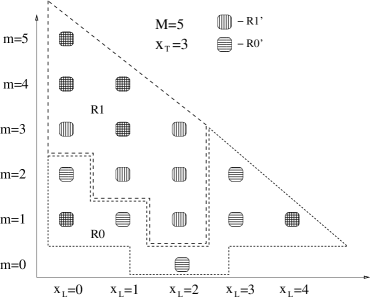
Denote by ρ(t|sinit)𝜌conditional𝑡subscript𝑠init\rho(t|s_{\rm init}) the first passage time density starting from some initial position sinit1subscript𝑠initsuperscript1s_{\rm init}\in\mathbb{R}1^{\prime} or 0superscript0\mathbb{R}0^{\prime}, see Fig. 5. The survival time density ϕ(t)italic-ϕ𝑡\phi(t) and waiting time density ψ(t)𝜓𝑡\psi(t) are then given by sinitρ(t|sinit)f(sinit)subscriptsubscript𝑠init𝜌conditional𝑡subscript𝑠init𝑓subscript𝑠init\sum_{s_{\rm init}}\rho(t|s_{\rm init})f(s_{\rm init}), where f(sinit)𝑓subscript𝑠initf(s_{\rm init}) is the distribution of initial points 1absentsuperscript1\in\mathbb{R}1^{\prime} (for ϕ(t)italic-ϕ𝑡\phi(t)) or 0superscript0\mathbb{R}0^{\prime} (for ψ(t)𝜓𝑡\psi(t)). Following standard arguments (see, e.g, translo ) we can write the expression for ρ(t|sinit)𝜌conditional𝑡subscript𝑠init\rho(t|s_{\rm init}), and therefore ψ(t)𝜓𝑡\psi(t) and ϕ(t)italic-ϕ𝑡\phi(t), which becomes:

ψ(t)𝜓𝑡\displaystyle\psi(t) =\displaystyle= p0η¯pc¯pexp(η¯pt),subscript𝑝0subscript¯𝜂𝑝subscript¯𝑐𝑝subscript¯𝜂𝑝𝑡\displaystyle\sum_{p\in\mathbb{R}0}\bar{\eta}_{p}\bar{c}_{p}\exp(-\bar{\eta}_{p}t), (32a)
ϕ(t)italic-ϕ𝑡\displaystyle\phi(t) =\displaystyle= p1η¯pc¯pexp(η¯pt),subscript𝑝1subscript¯𝜂𝑝subscript¯𝑐𝑝subscript¯𝜂𝑝𝑡\displaystyle\sum_{p\in\mathbb{R}1}\bar{\eta}_{p}\bar{c}_{p}\exp(-\bar{\eta}_{p}t), (32b)

where

c¯p=sinitQ¯p(sinit)f(sinit)Peq(sinit)sQ¯p(s).subscript¯𝑐𝑝subscriptsubscript𝑠initsubscript¯𝑄𝑝subscript𝑠init𝑓subscript𝑠initsubscript𝑃eqsubscript𝑠initsubscript𝑠subscript¯𝑄𝑝𝑠\bar{c}_{p}=\sum_{s_{\rm init}}\frac{\bar{Q}_{p}(s_{\rm init})f(s_{\rm init})}{P_{\rm eq}(s_{\rm init})}\sum_{s}\bar{Q}_{p}(s). (33)

Here, s0(1)𝑠01s\in\mathbb{R}0(\mathbb{R}1) for ψ(t)𝜓𝑡\psi(t) (ϕ(t)italic-ϕ𝑡\phi(t)), and η¯psubscript¯𝜂𝑝\bar{\eta}_{p} and Q¯p(s)subscript¯𝑄𝑝𝑠\bar{Q}_{p}(s) are determined through the eigenvalue equation (21), which explicitly becomes in s𝑠s-space van_Kampen

s~𝒲(s,s~)Q¯p(s~)=η¯pQ¯p(s),subscript~𝑠𝒲𝑠~𝑠subscript¯𝑄𝑝~𝑠subscript¯𝜂𝑝subscript¯𝑄𝑝𝑠\sum_{\tilde{s}}\mathscr{W}(s,\tilde{s})\bar{Q}_{p}(\tilde{s})=-\bar{\eta}_{p}\bar{Q}_{p}(s), (34)

where s,s~1𝑠~𝑠1s,\tilde{s}\in\mathbb{R}1 when calculating the survival time density, and s,s~0𝑠~𝑠0s,\tilde{s}\in\mathbb{R}0 for the waiting time density.

Refer to caption
Figure 5: Schematic of the (xL,m)subscript𝑥𝐿𝑚(x_{L},m)-points, region \mathbb{R}1 (\mathbb{R}0), for which the stochastic variable takes the value I=1𝐼1I=1 (I=0𝐼0I=0). The boundary points regions 1superscript1\mathbb{R}1^{\prime} and 0superscript0\mathbb{R}0^{\prime} are also indicated. The illustration is for the case M=5𝑀5M=5 and xT=3subscript𝑥𝑇3x_{T}=3, with Δ=0Δ0\Delta=0.

The problem is now reduced to obtaining the distribution of initial points f(sinit)𝑓subscript𝑠initf(s_{\rm init}) such that agreement with the Gillespie time series (see Appendix A) is obtained for long times. We define the rate coefficients for jumps from the points in the boundary region \mathbb{R}1’ to \mathbb{R}0’ (see Figs. 3 and 5): t10(sinit)=tL+,subscript𝑡10subscript𝑠initsuperscriptsubscript𝑡𝐿t_{1\rightarrow 0}(s_{\rm init})=t_{L}^{+}, tR,superscriptsubscript𝑡𝑅t_{R}^{-}, or tGsuperscriptsubscript𝑡𝐺t_{G}^{-}, where sinit1subscript𝑠initsuperscript1s_{\rm init}\in\mathbb{R}1^{\prime}. Similarly, for jumps from the points in the boundary region \mathbb{R}0’ to 1superscript1\mathbb{R}1^{\prime} (sinit0subscript𝑠initsuperscript0s_{\rm init}\in\mathbb{R}0^{\prime}) we define: t01(sinit)=tL,subscript𝑡01subscript𝑠initsuperscriptsubscript𝑡𝐿t_{0\rightarrow 1}(s_{\rm init})=t_{L}^{-}, tR+,superscriptsubscript𝑡𝑅t_{R}^{+}, or tG+superscriptsubscript𝑡𝐺t_{G}^{+}. From the detailed balance condition we have that

𝗍10(s)Peq(s)=𝗍01(s)Peq(s),subscript𝗍10𝑠subscript𝑃eq𝑠subscript𝗍01superscript𝑠subscript𝑃eqsuperscript𝑠\mathsf{t}_{1\rightarrow 0}(s)P_{\rm eq}(s)=\mathsf{t}_{0\rightarrow 1}(s^{\prime})P_{\rm eq}(s^{\prime}), (35)

where s𝑠s and ssuperscript𝑠s^{\prime} are points in region \mathbb{R}1’ and \mathbb{R}0’ which are connected. For the the survival time density we then choose the distribution of initial points proportional to the stationary influx from region 00\mathbb{R}0’. Furthermore using the detailed balance condition and normalizing we have for the initial distribution in the I=1𝐼1I=1 state

f(sinit)=𝗍10(sinit)Peq(sinit)sinit𝗍10(sinit)Peq(sinit)𝑓subscript𝑠initsubscript𝗍10subscript𝑠initsubscript𝑃eqsubscript𝑠initsubscriptsubscript𝑠initsubscript𝗍10subscript𝑠initsubscript𝑃eqsubscript𝑠initf(s_{\rm init})=\frac{\mathsf{t}_{1\rightarrow 0}(s_{\rm init})P_{\rm eq}(s_{\rm init})}{\sum_{s_{\rm init}}\mathsf{t}_{1\rightarrow 0}(s_{\rm init})P_{\rm eq}(s_{\rm init})} (36)

Similarly for the initial distribution in the I=0 state:

f(sinit)=𝗍01(sinit)Peq(sinit)sinit𝗍01(sinit)Peq(sinit),𝑓subscript𝑠initsubscript𝗍01subscript𝑠initsubscript𝑃eqsubscript𝑠initsubscriptsubscript𝑠initsubscript𝗍01subscript𝑠initsubscript𝑃eqsubscript𝑠initf(s_{\rm init})=\frac{\mathsf{t}_{0\rightarrow 1}(s_{\rm init})P_{\rm eq}(s_{\rm init})}{\sum_{s_{\rm init}}\mathsf{t}_{0\rightarrow 1}(s_{\rm init})P_{\rm eq}(s_{\rm init})}, (37)

which, together with Eqs. (32a), (32b) and (33), determines ψ(t)𝜓𝑡\psi(t) and ϕ(t)italic-ϕ𝑡\phi(t). We below proceed to show the choices above for f(sinit)𝑓subscript𝑠initf(s_{\rm init}) satisfy ergodicity requirements.

Ergodicity requires that the ratio of times spent in the I=1 and I=0 state equals

Req=s1Peq(s)s0Peq(s).subscript𝑅eqsubscript𝑠1subscript𝑃eq𝑠subscript𝑠0subscript𝑃eq𝑠R_{\rm eq}=\frac{\sum_{s\in\mathbb{R}1}P_{\rm eq}(s)}{\sum_{s\in\mathbb{R}0}P_{\rm eq}(s)}. (38)

From Eq. (32b) we have that the mean survival time can be written according to:

τsurv=0tϕ(t)𝑑t=p(η¯p)1c¯p,subscript𝜏survsuperscriptsubscript0𝑡italic-ϕ𝑡differential-d𝑡subscript𝑝superscriptsubscript¯𝜂𝑝1subscript¯𝑐𝑝\tau_{\rm surv}=\int_{0}^{\infty}t\phi(t)dt=\sum_{p}(\bar{\eta}_{p})^{-1}\bar{c}_{p}, (39)

and identically for the mean waiting time τwaitsubscript𝜏wait\tau_{\rm wait}. We proceed by noticing that the eigenvalue equation (34) can be written as

s~(𝒲refl(s,s~)𝒲abs(s,s~))Q¯p(s~)=η¯pQ¯p(s),subscript~𝑠superscript𝒲refl𝑠~𝑠superscript𝒲abs𝑠~𝑠subscript¯𝑄𝑝~𝑠subscript¯𝜂𝑝subscript¯𝑄𝑝𝑠\sum_{\tilde{s}}\left(\mathscr{W}^{\rm refl}(s,\tilde{s})-\mathscr{W}^{\rm abs}(s,\tilde{s})\right)\bar{Q}_{p}(\tilde{s})=-\bar{\eta}_{p}\bar{Q}_{p}(s), (40)

where

𝒲abs(s,s~)=𝗍10(s)δs,s~δs,sinit,superscript𝒲abs𝑠~𝑠subscript𝗍10𝑠subscript𝛿𝑠~𝑠subscript𝛿𝑠subscript𝑠init\mathscr{W}^{\rm abs}(s,\tilde{s})=\mathsf{t}_{1\rightarrow 0}(s)\delta_{s,\tilde{s}}\delta_{s,s_{\rm init}}, (41)

with sinit1subscript𝑠initsuperscript1s_{\rm init}\in\mathbb{R}1^{\prime}, and 𝒲refl(s,s~)superscript𝒲refl𝑠~𝑠\mathscr{W}^{\rm refl}(s,\tilde{s}) satisfy s𝒲refl(s,s~)=0subscript𝑠superscript𝒲refl𝑠~𝑠0\sum_{s}\mathscr{W}^{\rm refl}(s,\tilde{s})=0. Summing Eq. (34) over s𝑠s and using the above identity we obtain

sQ¯p(s)=sinitη¯p1𝗍10(sinit)Q¯p(sinit)subscript𝑠subscript¯𝑄𝑝𝑠subscriptsubscript𝑠initsuperscriptsubscript¯𝜂𝑝1subscript𝗍10subscript𝑠initsubscript¯𝑄𝑝subscript𝑠init\sum_{s}\bar{Q}_{p}(s)=\sum_{s_{\rm init}}\bar{\eta}_{p}^{-1}\mathsf{t}_{1\rightarrow 0}(s_{\rm init})\bar{Q}_{p}(s_{\rm init}) (42)

which is a useful connection between quantities in the bulk (s1𝑠1s\in\mathbb{R}1) and at the boundary sinit1subscript𝑠initsuperscript1s_{\rm init}\in\mathbb{R}1^{\prime}. Applying this relation to the expressions for the survival time, Eqs. (33), (36), and (39), we find

τsurv=pss~Q¯p(s)Q¯p(s~)sinit𝗍10(sinit)Peq(sinit).subscript𝜏survsubscript𝑝subscript𝑠subscript~𝑠subscript¯𝑄𝑝𝑠subscript¯𝑄𝑝~𝑠subscriptsubscript𝑠initsubscript𝗍10subscript𝑠initsubscript𝑃eqsubscript𝑠init\tau_{\rm surv}=\frac{\sum_{p}\sum_{s}\sum_{\tilde{s}}\bar{Q}_{p}(s)\bar{Q}_{p}(\tilde{s})}{\sum_{s_{\rm init}}\mathsf{t}_{1\rightarrow 0}(s_{\rm init})P_{\rm eq}(s_{\rm init})}. (43)

Finally, using the completeness relation van_Kampen

pQ¯p(s)Q¯p(s~)Peq(s~)=δs,s~,subscript𝑝subscript¯𝑄𝑝𝑠subscript¯𝑄𝑝~𝑠subscript𝑃eq~𝑠subscript𝛿𝑠~𝑠\sum_{p}\frac{\bar{Q}_{p}(s)\bar{Q}_{p}(\tilde{s})}{P_{\rm eq}(\tilde{s})}=\delta_{s,\tilde{s}}, (44)

we see that

τsurv=s1Peq(s)sinit𝗍10(s)Peq(sinit).subscript𝜏survsubscript𝑠1subscript𝑃eq𝑠subscriptsubscript𝑠initsubscript𝗍10𝑠subscript𝑃eqsubscript𝑠init\tau_{\rm surv}=\frac{\sum_{s\in\mathbb{R}1}P_{\rm eq}(s)}{\sum_{s_{\rm init}}\mathsf{t}_{1\rightarrow 0}(s)P_{\rm eq}(s_{\rm init})}. (45)

In a similar fashion

τwait=s0Peq(s)sinit𝗍01(s)Peq(sinit),subscript𝜏waitsubscript𝑠0subscript𝑃eq𝑠subscriptsubscript𝑠initsubscript𝗍01𝑠subscript𝑃eqsubscript𝑠init\tau_{\rm wait}=\frac{\sum_{s\in\mathbb{R}0}P_{\rm eq}(s)}{\sum_{s_{\rm init}}\mathsf{t}_{0\rightarrow 1}(s)P_{\rm eq}(s_{\rm init})}, (46)

which, using the detailed balance condition, Eq. (35), shows that τsurv/τwait=Reqsubscript𝜏survsubscript𝜏waitsubscript𝑅eq\tau_{\rm surv}/\tau_{\rm wait}=R_{\rm eq}.

With the completeness relation (44) and Eq. (42) we find from Eqs. (33), (36), and (37) that c¯psubscript¯𝑐𝑝\bar{c}_{p} can be written

c¯p=η¯p[sQ¯p(s)]2pη¯p[sQ¯p(s)]2subscript¯𝑐𝑝subscript¯𝜂𝑝superscriptdelimited-[]subscript𝑠subscript¯𝑄𝑝𝑠2subscript𝑝subscript¯𝜂𝑝superscriptdelimited-[]subscript𝑠subscript¯𝑄𝑝𝑠2\bar{c}_{p}=\frac{\bar{\eta}_{p}[\sum_{s}\bar{Q}_{p}(s)]^{2}}{\sum_{p}\bar{\eta}_{p}[\sum_{s}\bar{Q}_{p}(s)]^{2}} (47)

which is the form given in Eq. (22c).

Refer to caption
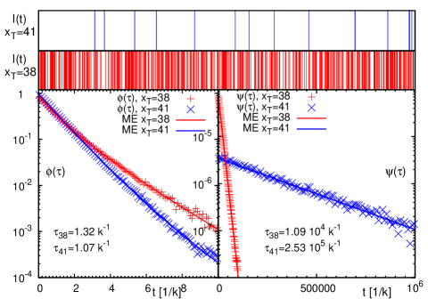
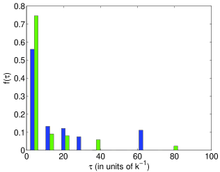
Figure 6: Top: Fluorescence time series I(t)𝐼𝑡I(t) for the T7 promoter sequence, with tag position xT=38subscript𝑥𝑇38x_{T}=38 (red) and xT=41subscript𝑥𝑇41x_{T}=41 (blue). Bottom: Waiting time (ψ(τ)𝜓𝜏\psi(\tau)) and fluorescence survival time (ϕ(τ)italic-ϕ𝜏\phi(\tau)) densities, in units of k𝑘k. The data points (solid lines) are results from the Gillespie algorithm (master equation). All results are for T=37C𝑇superscript37𝐶T=37^{\circ}C and 100 mM NaCl with DNA parameters from FK .

We show in Fig. 6 the time series obtained from a stochastic simulation (see Appendix A for a short introduction, and refer to Ref. suman for details) for two different tag positions in the T7 bacteriovirus promoter sequence

AAAA1AAAAAAAAAAAAAAAAAA20AAAA|AAAAAAAAAAAAAAAAAA|AAAAAAAAAAAA5’-aTGACCAGTTGAAGGACTGGAAGTAATACGACTCAAAAG TATAGGGACAATGCTTAAGGTCGCTCTCTAGGAg-3’AAAAAAA|AAAAAAAAAAAAAAAAAAAAAAAAAAA|AAAAAAAAAA38A41AAAAAAAAAAAAAAAAAAAAAAAAA68AAAAAAA1AAAAAAAAAAAAAAAAAA20AAAA|AAAAAAAAAAAAAAAAAA|AAAAAAAAAAAA5’-aTGACCAGTTGAAGGACTGGAAGTAATACGACTCAAAAG TATAGGGACAATGCTTAAGGTCGCTCTCTAGGAg-3’AAAAAAA|AAAAAAAAAAAAAAAAAAAAAAAAAAA|AAAAAAAAAA38A41AAAAAAAAAAAAAAAAAAAAAAAAA68AAA\begin{array}[]{l}\mbox{\small{{\color[rgb]{1,1,1}AAAA}1{\color[rgb]{1,1,1}AAAAAAAAAAAAAAAAAA}20}}\\[-4.26773pt] \mbox{\small{{\color[rgb]{1,1,1}AAAA}|{\color[rgb]{1,1,1}AAAAAAAAAAAAAAAAAA}|{\color[rgb]{1,1,1}AAAAAAAAA}{\color[rgb]{1,1,1}AAA}}}\\[-4.26773pt] \mbox{\small{5'-aTGACCAGTTGAAGGACTGGAAGTAATACGACTC}}\\ \mbox{\small{{\color[rgb]{1,1,1}AAA}AG}{\color[rgb]{1,0,0} {TATA}}{GGGACAATGCTTAAGGTCGCTCTCTAGGAg-3'}}\\[-4.26773pt] \mbox{\small{{\color[rgb]{1,1,1}AAAAAAA}|{\color[rgb]{1,1,1}AA}| {\color[rgb]{1,1,1}AAAAAAAAAAAAAAAAAAAAAAAAA}|{\color[rgb]{1,1,1}AAA}}}\\[-4.26773pt] \mbox{\small{{\color[rgb]{1,1,1}AAAAAAA}{\color[rgb]{1,0,0}38}{\color[rgb]{1,1,1}A}{\color[rgb]{0,0,1}41}{\color[rgb]{1,1,1}AAAAAAAAAAAAAAAAAAAAAAAAA}68{\color[rgb]{1,1,1}AAA}}}\end{array} (48)

whose TATA motif is marked in red Kalosakas_Rasmussen . A promoter is a sequence (often containing the so called TATA motif) marking the start of a gene, to which RNA polymerase is recruited and where transcription then initiates. Fig. 6 shows the signal I(t)𝐼𝑡I(t) at 37superscript3737^{\circ}C for the tag positions xT=38subscript𝑥𝑇38x_{T}=38 in the core of TATA, and xT=41subscript𝑥𝑇41x_{T}=41 at the second GC bp after TATA. Bubble events occur much more frequently in TATA (the TA/AT stacking interaction is particularly weak FK ). This is quantified by the density of waiting times ψ(τ)𝜓𝜏\psi(\tau) spent in the I=0𝐼0I=0 state, whose characteristic time scale τ=0𝑑ττψ(τ)superscript𝜏superscriptsubscript0differential-d𝜏𝜏𝜓𝜏\tau^{\prime}=\int_{0}^{\infty}d\tau\tau\psi(\tau) is more than an order of magnitude longer than at xT=41subscript𝑥𝑇41x_{T}=41. In contrast, we observe similar behavior for the density of opening times ϕ(τ)italic-ϕ𝜏\phi(\tau) for xT=38subscript𝑥𝑇38x_{T}=38 and 414141. The solid lines are the results from the master equation, see subsection III.2, showing excellent agreement with the Gillespie results. Notice that whereas ψ(t)𝜓𝑡\psi(t) is characterized by a single exponential, ϕ(t)italic-ϕ𝑡\phi(t) show a crossover between different regimes. For long times both ψ(τ)𝜓𝜏\psi(\tau) and ϕ(τ)italic-ϕ𝜏\phi(\tau) decay exponentially as it should for a finite DNA stretch.

V Reduced one-variable scheme for a homopolymer

After addressing the derivation of the probability densities ψ(t)𝜓𝑡\psi(t) and ϕ(t)italic-ϕ𝑡\phi(t), and the details concerning the transfer matrix 𝒲𝒲\mathscr{W}, we show how the master equation formalism reduces when a homopolymer sequence is considered, that is, a sequence with only one type of bps such as (AT)Nsubscript𝐴𝑇𝑁(AT)_{N}. Homopolymers can be realized experimentally. In the case they are clamped, possible secondary structure formation does not appear to occur, and our formalism remains valid. In the case of long homopolymers, imperfect matching conditions apply, and additional degrees of freedom emerge poland . Although this can be straightforwardly included in the formalism, we do not consider this case here.

In the homopolymer case, it is possible to obtain analytical results. To that end we note that for a homopolymer, all bps have the same statistical weights ust(x)subscript𝑢st𝑥u_{\mathrm{st}}(x) and uhb(x)subscript𝑢hb𝑥u_{\mathrm{hb}}(x). Formally, we therefore use u=ustuhb𝑢subscript𝑢stsubscript𝑢hbu=u_{\mathrm{st}}u_{\mathrm{hb}} for disruption of additional bps after bubble initiation. Due to this choice, we need to utilize the initiation factor σ0subscript𝜎0\sigma_{0} instead of the ring factor ξ𝜉\xi, as σ0subscript𝜎0\sigma_{0} takes care of the fact that upon initiation two stacking bonds are broken blake ; santalucia ; FK . If we furthermore assume that we are below the melting temperature u<1𝑢1u<1, have a long DNA region M1much-greater-than𝑀1M\gg 1 and consider bubbles far from the clamping, end effects are much less pronounced. It then follows that P(xL,m,t;xL,m)=P~(m,t;m)𝑃subscript𝑥𝐿𝑚𝑡superscriptsubscript𝑥𝐿superscript𝑚~𝑃𝑚𝑡superscript𝑚P(x_{L},m,t;x_{L}^{\prime},m^{\prime})=\tilde{P}(m,t;m^{\prime}), and the master equation reduces to

tP~(m,t)𝑡~𝑃𝑚𝑡\displaystyle\frac{\partial}{\partial t}\tilde{P}(m,t) =\displaystyle= 𝗍~+(m1)P~(m1,t)superscript~𝗍𝑚1~𝑃𝑚1𝑡\displaystyle\tilde{\mathsf{t}}^{+}(m-1)\tilde{P}(m-1,t) (49)
+𝗍~(m+1)P~(m+1,t)superscript~𝗍𝑚1~𝑃𝑚1𝑡\displaystyle+\tilde{\mathsf{t}}^{-}(m+1)\tilde{P}(m+1,t)
(𝗍~+(m)+𝗍~(m))P~(m,t),superscript~𝗍𝑚superscript~𝗍𝑚~𝑃𝑚𝑡\displaystyle-(\tilde{\mathsf{t}}^{+}(m)+\tilde{\mathsf{t}}^{-}(m))\tilde{P}(m,t),

with the short-hand notation P~(m,t)=P~(m,t;m)~𝑃𝑚𝑡~𝑃𝑚𝑡superscript𝑚\tilde{P}(m,t)=\tilde{P}(m,t;m^{\prime}). The forward transfer coefficients in this limit are given by

𝗍~+(m=0)superscript~𝗍𝑚0\displaystyle\tilde{\mathsf{t}}^{+}(m=0) =\displaystyle= kσ0us(0)𝑘subscript𝜎0𝑢𝑠0\displaystyle k\sigma_{0}us(0)
𝗍~+(m)|m1evaluated-atsuperscript~𝗍𝑚𝑚1\displaystyle\tilde{\mathsf{t}}^{+}(m)|_{m\geq 1} =\displaystyle= kus(m),𝑘𝑢𝑠𝑚\displaystyle kus(m), (50)

where we have incorporated the fact that a bubble size increase can occur by opening of a bp at either the left or the right fork. For the backward transfer coefficients, we find

𝗍~(m)=k.superscript~𝗍𝑚𝑘\tilde{\mathsf{t}}^{-}(m)=k. (51)

The eigenvalue equation corresponding to Eq. (49) has the comparatively simple structure

𝗍~+(m1)Q~p(m1)superscript~𝗍𝑚1subscript~𝑄𝑝𝑚1\displaystyle\tilde{\mathsf{t}}^{+}(m-1)\tilde{Q}_{p}(m-1)
+𝗍~(m+1)Q~p(m+1)superscript~𝗍𝑚1subscript~𝑄𝑝𝑚1\displaystyle+\tilde{\mathsf{t}}^{-}(m+1)\tilde{Q}_{p}(m+1)
(𝗍~+(m)+𝗍~(m))Q~p(m)=η~pQ~p(m),superscript~𝗍𝑚superscript~𝗍𝑚subscript~𝑄𝑝𝑚subscript~𝜂𝑝subscript~𝑄𝑝𝑚\displaystyle-(\tilde{\mathsf{t}}^{+}(m)+\tilde{\mathsf{t}}^{-}(m))\tilde{Q}_{p}(m)=-\tilde{\eta}_{p}\tilde{Q}_{p}(m), (52)

with eigenvalues η~psubscript~𝜂𝑝\tilde{\eta}_{p} and eigenvectors Q~p(m)subscript~𝑄𝑝𝑚\tilde{Q}_{p}(m) (p=0,1,,M𝑝01𝑀p=0,1,\ldots,M). The equation above is identical to the one in PRL ; JPC , and thus our generalized formalism is consistent with previous homopolymer models PRL ; JPC . We note that the equilibrium distribution becomes

P~eq(m)=𝒵(m)m=0M𝒵(m),subscript~𝑃eq𝑚𝒵𝑚superscriptsubscript𝑚0𝑀𝒵𝑚\tilde{P}_{\rm eq}(m)=\frac{\mathscr{Z}(m)}{\sum_{m=0}^{M}\mathscr{Z}(m)}, (53)

where 𝒵(m)=σ0(1+m)cum𝒵𝑚subscript𝜎0superscript1𝑚𝑐superscript𝑢𝑚\mathscr{Z}(m)=\sigma_{0}(1+m)^{-c}u^{m} with 𝒵(0)=1𝒵01\mathscr{Z}(0)=1, see Eqs. (1) and (2).

The autocorrelation function is, as before, simply proportional to the joint probability of having m1𝑚1m\geq 1 at time t𝑡t and m1𝑚1m\geq 1 at initial time t=0𝑡0t=0. Proceeding as previously, and assuming that initially the system is at equilibrium, P(m,0;m,0)=δmmP~eq(m)𝑃𝑚0superscript𝑚0subscript𝛿𝑚superscript𝑚subscript~𝑃eq𝑚P(m,0;m^{\prime},0)=\delta_{mm^{\prime}}\tilde{P}_{\rm eq}(m), we have

A~(t)=I(t)I(0)(I)2=p0(T~p)2exp(tτ~p),~𝐴𝑡delimited-⟨⟩𝐼𝑡𝐼0superscriptdelimited-⟨⟩𝐼2subscript𝑝0superscriptsubscript~𝑇𝑝2𝑡subscript~𝜏𝑝\tilde{A}(t)=\langle I(t)I(0)\rangle-(\langle I\rangle)^{2}=\sum_{p\neq 0}\left(\tilde{T}_{p}\right)^{2}\exp\left(-\frac{t}{\tilde{\tau}_{p}}\right), (54)

where T~p=m=1MQ~p(m)subscript~𝑇𝑝superscriptsubscript𝑚1𝑀subscript~𝑄𝑝𝑚\tilde{T}_{p}=\sum_{m=1}^{M}\tilde{Q}_{p}(m). Here, we introduced the relaxation times τ~p1/η~psubscript~𝜏𝑝1subscript~𝜂𝑝\tilde{\tau}_{p}\equiv 1/\tilde{\eta}_{p}. As before, we write the correlation function according to A~(t)=𝑑τexp(t/τ)f~(τ)~𝐴𝑡differential-d𝜏𝑡𝜏~𝑓𝜏\tilde{A}(t)=\int d\tau\exp(-t/\tau)\tilde{f}(\tau), with the relaxation time spectrum

f~(τ)=p0(T~p)2δ(ττ~p).~𝑓𝜏subscript𝑝0superscriptsubscript~𝑇𝑝2𝛿𝜏subscript~𝜏𝑝\tilde{f}(\tau)=\sum_{p\neq 0}\left(\tilde{T}_{p}\right)^{2}\delta(\tau-\tilde{\tau}_{p}). (55)
Refer to caption
Refer to caption
Refer to caption
Refer to caption
Refer to caption
Refer to caption
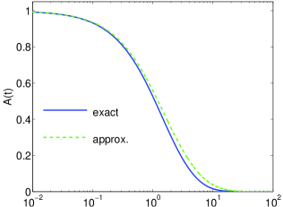
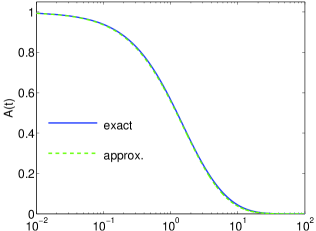
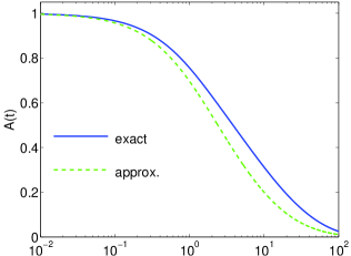
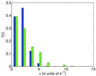
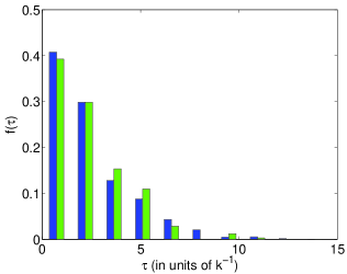
Figure 7: Autocorrelation A(t)𝐴𝑡A(t) and spectral density f(τ)𝑓𝜏f(\tau) for a tagged bp in a homopolymer region: u=uhb𝑢subscript𝑢hbu=u_{\rm hb}ustsubscript𝑢stu_{\rm st}. Left: Close-to-end-tagging far from Tmsubscript𝑇𝑚T_{m} (xT=2subscript𝑥𝑇2x_{T}=2, u=0.6𝑢0.6u=0.6). Middle: Center-tagging far from Tmsubscript𝑇𝑚T_{m} (xT=20subscript𝑥𝑇20x_{T}=20, u=0.6𝑢0.6u=0.6). Right: Center-tagging close to Tmsubscript𝑇𝑚T_{m} (xT=20subscript𝑥𝑇20x_{T}=20, u=0.9𝑢0.9u=0.9). In the A(t)𝐴𝑡A(t) plots the blue curves are the exact result. The dashed green curves are approximated from from Eqs. (52) and (54). In the spectral density plot the data were collected into 10 bins. The green bars are the approximate one-variable results, Eq. (55), and the blue bars are the exact result. The length of the DNA segment was M=40𝑀40M=40. The approximate expression only works well for internal tagging and below Tmsubscript𝑇𝑚T_{m}.

In Fig. 7, we compare the approximate result for A(xT,t)𝐴subscript𝑥𝑇𝑡A(x_{T},t) obtained by numerical solution of Eqs. (52), and using Eq. (54), with the general result from the master equation in Section III. We also show the corresponding weighted spectral densities given by Eq. (55). We note that the approximate expression works well only for the case of internal tagging and temperatures below the melting temperature (and for a sufficiently long DNA region); for a short DNA sequence, close-to-end-tagging or high temperatures (i.e., large bubbles) end effects, which are not included in the approximate model above, are significant.

In the analysis of Refs. PRL ; bj it was found that close to the melting transition at Tmsubscript𝑇𝑚T_{m}, the mean correlation function takes its maximum (critical slowing down). In order to get an understanding of this behavior we here analytically obtain the largest relaxation time from the homopolymer model above. From Reference tobias we have that the eigenvalues, see Eq. (52), are for c=0𝑐0c=0

η~p=k(u+12u1/2cosωp)subscript~𝜂𝑝𝑘𝑢12superscript𝑢12subscript𝜔𝑝\tilde{\eta}_{p}=k(u+1-2u^{1/2}\cos\omega_{p}) (56)

where ωpsubscript𝜔𝑝\omega_{p} (0<ωpπ0subscript𝜔𝑝𝜋0<\omega_{p}\leq\pi) is obtained from the transcendental equation

g(ωp)=sin[(M+1)ωp]δsin[Mωp]=0𝑔subscript𝜔𝑝𝑀1subscript𝜔𝑝𝛿𝑀subscript𝜔𝑝0g(\omega_{p})=\sin[(M+1)\omega_{p}]-\delta\sin[M\omega_{p}]=0 (57)

with δ=(1σ0)u1/2𝛿1subscript𝜎0superscript𝑢12\delta=(1-\sigma_{0})u^{1/2}. For u1𝑢1u\rightarrow 1 and σ00subscript𝜎00\sigma_{0}\rightarrow 0 we get

g(ωp)𝑔subscript𝜔𝑝\displaystyle g(\omega_{p}) =\displaystyle= sin[(M+1)ωp]sin[Mωp]𝑀1subscript𝜔𝑝𝑀subscript𝜔𝑝\displaystyle\sin[(M+1)\omega_{p}]-\sin[M\omega_{p}] (58)
=\displaystyle= 2sinωp2cos[(M+12)ωp]2subscript𝜔𝑝2𝑀12subscript𝜔𝑝\displaystyle 2\sin\frac{\omega_{p}}{2}\cos[(M+\frac{1}{2})\omega_{p}]

so that we have

ωp=(p1/2)πM+1/2subscript𝜔𝑝𝑝12𝜋𝑀12\omega_{p}=\frac{(p-1/2)\pi}{M+1/2} (59)

which together with Eq. (56) give the eigenvalues. The smallest eigenvalue (largest relaxation time) is obtained for p=1𝑝1p=1, i.e. η~1=2k(1cos(π/[2M+1]))kπ2/(2M+1)2subscript~𝜂12𝑘1𝜋delimited-[]2𝑀1𝑘superscript𝜋2superscript2𝑀12\tilde{\eta}_{1}=2k(1-\cos(\pi/[2M+1]))\approx k\pi^{2}/(2M+1)^{2} for M1much-greater-than𝑀1M\gg 1, and therefore the largest relaxation time becomes

τ~1=1η~1(2M+1)2π2k1subscript~𝜏11subscript~𝜂1superscript2𝑀12superscript𝜋2superscript𝑘1\tilde{\tau}_{1}=\frac{1}{\tilde{\eta}_{1}}\approx\frac{(2M+1)^{2}}{\pi^{2}}k^{-1} (60)

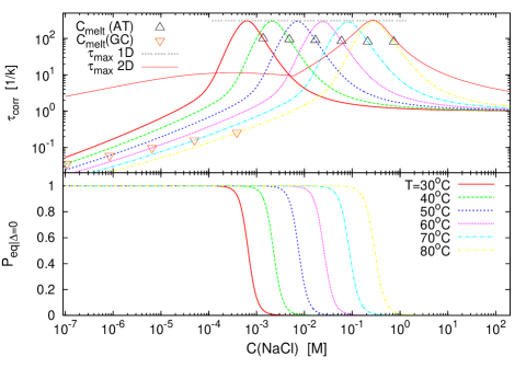
We notice that the longest relaxation time scales as M2similar-toabsentsuperscript𝑀2\sim M^{2} at melting, in agreement with the findings in bicout . Fig. 8 demonstrates the good agreement of the homopolymer result (τmaxsubscript𝜏max\tau_{\mathrm{max}}, 1D in the figure) with the maxima of the correlation time, that coincide with the melting concentration.
Refer to caption
Figure 8: Top: Mean correlation time τcorr=0𝑑tA(t)/A(0)subscript𝜏corrsuperscriptsubscript0differential-dsuperscript𝑡𝐴superscript𝑡𝐴0\tau_{\rm corr}=\int_{0}^{\infty}dt^{\prime}A(t^{\prime})/A(0) versus NaCl concentration for various temperatures T𝑇T for the AT9 construct of Ref. altan , showing a critical slowing down at the melting concentration (compare lower panel). The triangles denotes the melting concentration for infinitely long random AT and GC stretches. The curve denoted by τmax1Dsubscript𝜏max1𝐷\tau_{{\rm max}1D} is the result given in Eq. (60), and τmax2D=max{τp}subscript𝜏max2𝐷subscript𝜏𝑝\tau_{{\rm max}2D}=\max\{\tau_{p}\}, p=1,,S𝑝1𝑆p=1,\ldots,S is the maximum relaxation time of the full problem specified in Sec. III. Bottom: Opening probability of bp xTsubscript𝑥𝑇x_{T}.

VI Conclusions

In this study we considered the bubble breathing dynamics in a heteropolymer DNA-region characterized by statistical weights ust(x)subscript𝑢st𝑥u_{\rm st}(x) for disrupting a stacking interaction between neighboring bps, and the weight uhb(x)subscript𝑢hb𝑥u_{\rm hb}(x) for breaking a Watson-Crick hydrogen bond (x𝑥x labels different bps), as well the bubble initiation parameter (the ring-factor) σ0subscript𝜎0\sigma_{0} (ξ𝜉\xi). For that purpose, we introduced a (2+1)21(2+1)-variable master equation governing the time evolution of the probability distribution to find a bubble of size m𝑚m with left fork position xLsubscript𝑥𝐿x_{L} at time t𝑡t, as well as a complementary Gillespie scheme. The time averages from the stochastic simulation agree well with the ensemble properties derived from the ME. We calculate the spectrum of relaxation times, and in particular the experimentally measurable autocorrelation function of a tagged bp is obtained. All parameters in our model are known from recent equilibrium measurements available for a wide range of temperatures and NaCl concentrations, except for the rate constant k𝑘k for (un)zipping that is the only free fit parameter. A better understanding of the zipping rate k𝑘k remains an open question, requiring a detailed microscopic modelling of DNA-breathing.

For the case of a long homopolymer DNA region with internal tagging and below the melting temperature the position of the bubble becomes negligible, and the master equation reduces to previous (1+1)-variable approaches in terms of the bubble size.

Acknowledgements.
We thank Maxim Frank-Kamenetskii, Oleg Krichevsky, and Kim Splitorff for very helpful discussion. SKB acknowledges support from Virginia Tech through ASPIRES award program. TA acknowledges partial support through a Research Career Award from the Knut and Alice Wallenberg foundation. RM acknowledges partial funding from the Natural Sciences and Engineering Research Council (NSERC) of Canada and the Canada Research Chairs program.

Appendix A Gillespie approach

In this section we briefly review the Gillespie algorithm. Together with the explicit expressions for the transfer coefficients introduced in the previous section it is used to generate stochastic time series of bubble breathing. In particular we show how the motion of a tagged bp is obtained.

To denote a bubble state of m𝑚m broken bps at position xLsubscript𝑥𝐿x_{L} we define the occupation number b(xL,m)𝑏subscript𝑥𝐿𝑚b(x_{L},m) for each lattice point in Fig. 3 with the properties b(xL,m)=1𝑏subscript𝑥𝐿𝑚1b(x_{L},m)=1 if the particular state {xL,m}subscript𝑥𝐿𝑚\{x_{L},m\} is occupied and b(xL,m)=0𝑏subscript𝑥𝐿𝑚0b(x_{L},m)=0 for unoccupied states. For the completely zipped state m=0𝑚0m=0 there is no dependence on xLsubscript𝑥𝐿x_{L}, and we introduce the occupation number b(0)𝑏0b(0). The stochastic DNA breathing then corresponds to the nearest neighbor jump processes in the triangular lattice in Fig. 3. Each jump away from the state {xL,m}subscript𝑥𝐿𝑚\{x_{L},m\} (i.e., from the state with b(xL,m)=1𝑏subscript𝑥𝐿𝑚1b(x_{L},m)=1) occurs at a random time τ𝜏\tau and in a random direction to one of the nearest neighbors; it is governed by the reaction probability density function Gillespie ; Gillespie1

P(τ,μ,ν)=𝗍νμ(xL,m)exp(τμ,ν𝗍νμ(xL,m)),𝑃𝜏𝜇𝜈subscriptsuperscript𝗍𝜇𝜈subscript𝑥𝐿𝑚𝜏subscript𝜇𝜈subscriptsuperscript𝗍𝜇𝜈subscript𝑥𝐿𝑚P(\tau,\mu,\nu)=\mathsf{t}^{\mu}_{\nu}(x_{L},m)\exp\left(-\tau\sum_{\mu,\nu}\mathsf{t}^{\mu}_{\nu}(x_{L},m)\right), (61)

which for a given state (xL,m)subscript𝑥𝐿𝑚(x_{L},m) defines after what waiting time τ𝜏\tau the next step occurs and in what ’direction’, ν{G,L,R}𝜈𝐺𝐿𝑅\nu\in\{G,L,R\}, μ{+/}\mu\in\{+/-\}. A simulation run produces a time series of occupied states {xL,m}subscript𝑥𝐿𝑚\{x_{L},m\} and how long time τ=τj𝜏subscript𝜏𝑗\tau=\tau_{j} (j=1,,N𝑗1𝑁j=1,...,N, where N𝑁N is the number of steps in the simulation) this particular state is occupied. This waiting time τ𝜏\tau, that is, according to Eq. (61) follows a Poisson distribution cox .

A.1 Tagged bp survival and waiting time densities

The stochastic variable I(t)𝐼𝑡I(t) is then obtained by summing the Gillespie occupation number b(xL,m)𝑏subscript𝑥𝐿𝑚b(x_{L},m) (b(xL,m)𝑏subscript𝑥𝐿𝑚b(x_{L},m) takes only values 00 or 111) over region 11\mathbb{R}1, i.e.

I(t)=xL,m1b(xL,m).𝐼𝑡subscriptsubscript𝑥𝐿𝑚1𝑏subscript𝑥𝐿𝑚I(t)=\sum_{x_{L},m\in\mathbb{R}1}b(x_{L},m). (62)

From the time series for I(t)𝐼𝑡I(t) one can, for instance, calculate the waiting time distribution ψ(τ)𝜓𝜏\psi(\tau) of times spent in the I=0𝐼0I=0 state, as well as the survival time distribution ϕ(τ)italic-ϕ𝜏\phi(\tau) of times in the I=1𝐼1I=1 state. Explicit examples for ψ(τ)𝜓𝜏\psi(\tau) and ϕ(τ)italic-ϕ𝜏\phi(\tau) are shown in Sec. IV.

The probability that the tagged bp is open becomes

PG(tj)=1tNj=1NτjI(tj)subscript𝑃𝐺subscript𝑡𝑗1subscript𝑡𝑁superscriptsubscript𝑗1𝑁subscript𝜏𝑗𝐼subscript𝑡𝑗P_{G}(t_{j})=\frac{1}{t_{N}}\sum_{j=1}^{N}\tau_{j}I(t_{j}) (63)

where tj=j=1jτjsubscript𝑡𝑗superscriptsubscriptsuperscript𝑗1𝑗subscript𝜏superscript𝑗t_{j}=\sum_{j^{\prime}=1}^{j}\tau_{j^{\prime}}. For long times the explicit construction of the Gillespie scheme together with the detailed balance conditions guarantee that PG(tj)subscript𝑃𝐺subscript𝑡𝑗P_{G}(t_{j}) tends to the equilibrium probability, i.e. that PG(tj)=xL,m1Peq(xL,m)subscript𝑃𝐺subscript𝑡𝑗subscriptsubscript𝑥𝐿𝑚1superscript𝑃eqsubscript𝑥𝐿𝑚P_{G}(t_{j}\rightarrow\infty)=\sum_{x_{L},m\in\mathbb{R}1}P^{\rm eq}(x_{L},m), where Peq(xL,m)superscript𝑃eqsubscript𝑥𝐿𝑚P^{\rm eq}(x_{L},m) is given in Eq. (2).

A.2 Tagged base-pair autocorrelation function

The autocorrelation function for a tagged bp is obtained through

At(xT,t)subscript𝐴𝑡subscript𝑥𝑇𝑡\displaystyle A_{t}(x_{T},t) =\displaystyle= I(t)I(0)¯(I(t)¯)2¯𝐼𝑡𝐼0superscript¯𝐼𝑡2\displaystyle\overline{I(t)I(0)}-(\overline{I(t)})^{2} (64)
=1T0TI(t+t)I(t)𝑑t(1T0TI(t)𝑑t)2absent1𝑇superscriptsubscript0𝑇𝐼𝑡superscript𝑡𝐼superscript𝑡differential-dsuperscript𝑡superscript1𝑇superscriptsubscript0𝑇𝐼superscript𝑡differential-dsuperscript𝑡2\displaystyle=\frac{1}{T}\int_{0}^{T}I(t+t^{\prime})I(t^{\prime})dt^{\prime}-\left(\frac{1}{T}\int_{0}^{T}I(t^{\prime})dt^{\prime}\right)^{2}

which for long times agrees with the the ensemble average, Eq. (14), from the master equation. The function At(xT,t)subscript𝐴𝑡subscript𝑥𝑇𝑡A_{t}(x_{T},t) corresponds to the blinking autocorrelation function obtained in the FCS experiment from Ref. altan .

References

  • (1) A. Kornberg, DNA Synthesis (W. H. Freeman, San Francisco, CA, 1974).
  • (2) D. Poland and H. A. Scheraga, Theory of Helix-Coil Transitions in Biopolymers (Academic Press, New York, 1970).
  • (3) R. M. Wartell and A. S. Benight, Phys. Rep. 126, 67 (1985).
  • (4) C. R. Cantor and P. R. Schimmel, Biophysical Chemistry, Part 3 (W. H. Freeman, New York, 1980).
  • (5) Note that for T=37𝑇superscript37T=37^{\circ}C we used that 1kBT=0.621subscript𝑘𝐵𝑇0.621k_{B}T=0.62kcal/mol. Also note that writing Boltzmann factors for the free energies as exp(βΔG)𝛽Δ𝐺\exp(\beta\Delta G), with β=1/(kBT)𝛽1subscript𝑘𝐵𝑇\beta=1/(k_{B}T), a positive ΔGΔ𝐺\Delta G denotes an unstable bond.
  • (6) R. D. Blake, J. W. Bizzaro, J. D. Blake, G. R. Day, S. G. Delcourt, J. Knowles, K. A. Marx, and J. SantaLucia Jr., Bioinformatics 15, 370 (1999).
  • (7) R. Blossey and E. Carlon, Phys. Rev. E 68, 061911 (2003).
  • (8) A. Krueger, E. Protozanova, and M. D. Frank-Kamenetskii, Biophys. J. 90, 3091 (2006).
  • (9) E. Protozanova, P. Yakovchuk, and M. D. Frank-Kamenetskii, J. Mol. Biol. 342, 775 (2004).
  • (10) M. Guéron, M. Kochoyan, and J.-L. Leroy, Nature 328, 89 (1987).
  • (11) G. Altan-Bonnet, A. Libchaber, and O. Krichevsky, Phys. Rev. Lett. 90, 138101 (2003).
  • (12) K. Pant, R. L. Karpel, and M. C. Williams, J. Mol. Biol. 327, 571 (2003).
  • (13) K. Pant, R. L. Karpel, I. Rouzina, and M. C. Williams, J. Mol. Biol. 336, 851 (2004).
  • (14) R. L. Karpel, IUBMB Life 53, 161 (2002).
  • (15) T. Ambjörnsson and R. Metzler, Phys. Rev. E 72, 030901(R) (2005).
  • (16) T. Ambjörnsson and R. Metzler, J. Phys. Cond. Mat. 17, S1841 (2005).
  • (17) T. Ambjörnsson, S. K. Banik, and R. Metzler, Biophys. J., submitted.
  • (18) M. Fixman and J. J. Freire, Biopol. 16, 2693 (1977).
  • (19) See C. Richard and A. J. Guttmann, J. Stat. Phys. 115, 925 (2004) and Refs. therein.
  • (20) H. Risken, The Fokker-Planck equation (Springer-Verlag, Berlin, 1989).
  • (21) Also, 𝗍L+(xL=1,m)=0superscriptsubscript𝗍𝐿subscript𝑥𝐿1𝑚0\mathsf{t}_{L}^{+}(x_{L}=-1,m)=0 and 𝗍R(xL,m=MxL+1)=0superscriptsubscript𝗍𝑅subscript𝑥𝐿𝑚𝑀subscript𝑥𝐿10\mathsf{t}_{R}^{-}(x_{L},m=M-x_{L}+1)=0 for m=2,,M+1𝑚2𝑀1m=2,...,M+1 for completeness.
  • (22) N. G. van Kampen, Stochastic Processes in Physics and Chemistry, 2nd Ed. (North-Holland, Amsterdam, 1992).
  • (23) C. W. Gardiner, Handbook of Stochastic Methods for Physics, Chemistry and the Natural Sciences (Springer, Berlin, 1989).
  • (24) T. Ambjörnsson, S. K. Banik, and R. Metzler, Phys. Rev. Lett. 97, 128105 (2006).
  • (25) E. A. Di Marzio, C. M. Guttman, and J. D. Hoffman, Faraday Disc. 68, 210 (1979).
  • (26) T. Ambjörnsson, M. A. Lomholt, and R. Metzler, J. Phys. Cond. Mat. 17, S3945 (2005).
  • (27) S. K. Banik, T. Ambjörnsson, and R. Metzler, Europhys. Lett. 71, 852 (2005).
  • (28) G. Kalosakas, K. Ø. Rasmussen, A. R. Bishop, C. H. Choi, and A. Usheva, Europhys. Lett. 68, 127 (2004).
  • (29) J. SantaLucia Jr., Proc. Natl. Acad. Sci. USA 95, 1460 (1998).
  • (30) D. J. Bicout and E. Kats, Phys. Rev. E 70, 010902(R) (2004).
  • (31) D. T. Gillespie, J. Comp. Phys. 22, 403 (1976).
  • (32) D. T. Gillespie, J. Phys. Chem. 81 2340 (1977).
  • (33) D. R. Cox, Renewal Theory (J. Wiley & Sons, New York, NY, 1962).