Present address: ]Department of Physics, Massachusetts Institute of Technology, Cambridge, MA 02139, USA

Correlation-Induced Resonances and Population Switching in a Quantum Dot Coulomb Valley

Abstract

Strong correlation effects on electron transport through a spinless quantum dot are considered. When two single-particle levels in the quantum dot are degenerate, a conserved pseudospin degree of freedom appears for generic tunneling matrix elements between the quantum dot and leads. Local fluctuations of the pseudospin in the quantum dot give rise to a pair of asymmetric conductance peaks near the center of a Coulomb valley. An exact relation to the population switching is provided.

Introduction.— Electronic transport through a quantum dot (QD) is a useful probe of the strong Coulomb interaction effects in zero dimensional systems Sohn97Book . One of well-known interaction effects is the Coulomb blockade Kastner93PT , which allows the current to flow through the QD only at special gate voltages and suppresses the current at other gate voltages (Coulomb valleys). The interaction also induces electronic correlations responsible for deviations from the orthodox Coulomb blockade theory Kastner93PT . In Coulomb valleys, the current may be enhanced by the spin fluctuations via the spin Kondo effect SpinKondoTh ; SpinKondoExp , or by the orbital fluctuations via the orbital Kondo effect OrbitalKondoTh ; Boese01PRB ; OrbitalKondoExp .

Recently an intriguing experimental report Schuster97Nature of the anomalous transmission phase through a QD motivated theoretical studies Silvestrov00PRL ; Sindel05PRB ; Kim06PRB ; Meden06PRL of the correlation effects in a spinless QD system with two single-particle levels [Fig. 1(a)]. In particular, the study Meden06PRL using the functional renormalization group method revealed that when the two levels are degenerate, the conductance through the QD is anomalously enhanced near the center of a Coulomb valley and forms a pair of asymmetric peaks. These peaks are termed as correlation-induced resonances (CIRs). The nature of the correlation, however, remains unclear. The spin Kondo effect SpinKondoTh ; SpinKondoExp is not applicable since the system is spinless. The orbital Kondo effect in Refs. OrbitalKondoTh ; Boese01PRB ; OrbitalKondoExp is not applicable either since it occurs only when the tunneling matrix elements between the QD and leads satisfy certain constraints OrbitalKondoTh ; Boese01PRB while the CIRs appear for generic tunneling matrix elements. A possibly related phenomenon is the so-called population switching (PS) Silvestrov00PRL ; Sindel05PRB ; Kim06PRB ; Near the center of the Coulomb valley, the electron population of the QD switches from one single-particle level to the other. The relation between the CIRs and the PS also remains unclear however. In this Letter, (i) we show that the QD system with two single-particle levels possesses a conserved pseudospin degree of freedom when the two levels are degenerate, (ii) provide an exact relation between the CIRs and the PS, and (iii) demonstrate that local fluctuations of the pseudospin in the QD are the origin of the CIRs.

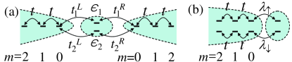
Figure 1: (Color online) (a) A quantum dot with two single-particle levels $\epsilon_{1}$, $\epsilon_{2}$ coupled to two leads. When $\epsilon_{1}=\epsilon_{2}$, the system may be transformed to a new system shown in (b).

The spinless QD system may be realized in experiments, for instance, when a QD with two orbital levels, each with the two-fold spin degeneracy, is subjected to a strong magnetic field. If the resulting Zeeman splitting is sufficiently larger than the energy difference of the two orbital levels, the transport through the QD in the Coulomb valley with only one electron in the QD can be described by the following spinless Hamiltonian Sindel05PRB ; Meden06PRL ,

$${\cal H}={\cal H}_{\rm dot}+{\cal H}_{\rm lead}+{\cal H}_{T},$$ (1)

where ${\cal H}_{\rm dot}\equiv\sum_{j=1}^{2}\epsilon_{j}d_{j}^{\dagger}d_{j}+U(n_{1}-1/2)(n_{2}-1/2)$, ${\cal H}_{\rm lead}\equiv-t\sum_{l=L,R}\sum^{\infty}_{m=0}(c^{\dagger}_{m,l}c_{m+1,l}+H.c.)$, ${\cal H}_{T}\equiv-\sum_{j,l}(t_{j}^{l}c_{0,l}^{\dagger}d_{j}+H.c.)$. Here $\epsilon_{j}$ denotes the energy of the single-particle state $j$ in the QD. $d_{j}$ and $c_{m,l}$ are the annihilation operators for the electron in the QD and for the electron at the site $m$ in the lead $l$, respectively. $n_{j}\equiv d^{\dagger}_{j}d_{j}$. Note that each lead contains only one channel [Fig. 1(a)]. This is motivated by the experimental situation in Ref. Schuster97Nature , where narrow constrictions are introduced between a QD and leads in order to force the system into the single channel regime.

Pseudospin.— The pseudospin degree of freedom can be revealed by the following unitary transformations from $c_{m,L(R)}$, $d_{1(2)}$ to the new operators $c_{m,\uparrow(\downarrow)}$, $d_{\uparrow(\downarrow)}$,

$$\left(\begin{array}[]{cc}c_{m,\uparrow}\\ c_{m,\downarrow}\end{array}\right)\!=\!{\cal U}_{\rm lead}\!\left(\!\begin{array}[]{cc}c_{m,L}\\ c_{m,R}\end{array}\!\right), {\cal U}_{\rm lead}=\left(\begin{array}[]{cc}\eta&\zeta^{*}\\ \zeta&-\eta^{*}\end{array}\right),$$ (8)

$$\left(\begin{array}[]{cc}d_{\uparrow}\\ d_{\downarrow}\end{array}\right)={\cal U}_{\rm dot}\left(\begin{array}[]{cc}d_{1}\\ d_{2}\end{array}\right), {\cal U}_{\rm dot}=\left(\begin{array}[]{cc}\alpha&\beta^{*}\\ \beta&-\alpha^{*}\end{array}\right),$$ (15)

under which ${\cal H}_{\rm lead}$ remains invariant for general $\alpha$, $\beta$, $\eta$, $\zeta$ with $\left|\alpha\right|^{2}+\left|\beta\right|^{2}=\left|\eta\right|^{2}+\left|\zeta\right|^{2}=1$. When the two dot levels are degenerate $\epsilon_{1}=\epsilon_{2}=\epsilon$, ${\cal H}_{\rm dot}$ transforms to ${\cal H}_{\rm dot}^{\rm(1)}\equiv\sum_{\sigma=\uparrow,\downarrow}\epsilon d_{\sigma}^{\dagger}d_{\sigma}+U(n_{\uparrow}-{1\over 2})(n_{\downarrow}-{1\over 2})$, and thus ${\cal H}_{\rm dot}$ also remains invariant. Finally ${\cal H}_{T}$ transforms to

$${\cal H}_{T}=-\left(\begin{array}[]{cc}c_{0,\uparrow}^{\dagger}&c_{0,\downarrow}^{\dagger}\end{array}\right)\Lambda\left(\begin{array}[]{cc}d_{\uparrow}\\ d_{\downarrow}\end{array}\right)+H.c.,$$ (16)

where $\Lambda\equiv{\cal U}_{\rm lead}T{\cal U}_{\rm dot}^{\dagger}$ and $T=\left(\begin{array}[]{cc}t_{1}^{L}&t_{2}^{L}\\ t_{1}^{R}&t_{2}^{R}\end{array}\right)$. We choose ${\cal U}_{\rm lead}$ and ${\cal U}_{\rm dot}$ in such a way that $\Lambda$ becomes diagonal with diagonal elements $\lambda_{\uparrow}$ and $\lambda_{\downarrow}$, i.e., ${\cal H}_{T}=-(\lambda_{\uparrow}c_{0,\uparrow}^{\dagger}d_{\uparrow}+\lambda_{\downarrow}c_{0,\downarrow}^{\dagger}d_{\downarrow}+H.c.)$. Such a diagonalization can be achieved for general $T$ by choosing ${\cal U}_{\rm lead}$ and ${\cal U}_{\rm dot}$ to be the solutions of the eigenvalue equations $(TT^{\dagger}){\cal U}_{\rm lead}^{\dagger}={\cal U}_{\rm lead}^{\dagger}(\Lambda^{\dagger}\Lambda)$ and $(T^{\dagger}T){\cal U}_{\rm dot}^{\dagger}={\cal U}_{\rm dot}^{\dagger}(\Lambda\Lambda^{\dagger})$. Without loss of generality, we may assume that both $\lambda_{\uparrow}$ and $\lambda_{\downarrow}$ are real and $\lambda_{\uparrow}\geq\lambda_{\downarrow}\geq 0$. Note that in the transformed system, the electron tunneling between the pseudospin $\uparrow$ states [upper half in Fig. 1(b)] and the pseudospin $\downarrow$ states (lower half) is prohibited. This illustrates the existence of the conserved pseudospin $\sigma$ ($\uparrow$ or $\downarrow$) for general $t_{j}^{l}$’s. This generalizes the earlier reports Boese01PRB ; Meden06PRL of the conserved pseudospin for special $t_{j}^{l}$’s, for which $\lambda_{\uparrow}=\lambda_{\downarrow}$ and the system possesses the SU(2) pseudospin symmetry. In contrast, the symmetry is reduced to U(1) when $\lambda_{\uparrow}\neq\lambda_{\downarrow}$. Later in this Letter, it will be demonstrated that the difference $\lambda_{\uparrow}\neq\lambda_{\uparrow}$ is crucial for the CIRs.

On the other hand, when the degeneracy is lifted $\epsilon_{1(2)}=\epsilon\pm\delta/2$, the original Hamiltonian [Eq. (1)] transforms to ${\cal H}_{\rm dot}^{(1)}+{\cal H}_{\rm dot}^{(2)}+{\cal H}_{\rm dot}^{(3)}+{\cal H}_{\rm lead}+{\cal H}_{T}$ under the transformations [Eqs. (8),(15)] that diagonalize $\Lambda$. Here the two additional terms ${\cal H}_{\rm dot}^{(2)}$ and ${\cal H}_{\rm dot}^{(3)}$ are defined as ${\cal H}_{\rm dot}^{(2)}\equiv\delta(|\alpha|^{2}-|\beta|^{2})(n_{\uparrow}-n_{\downarrow})/2$, and ${\cal H}_{\rm dot}^{(3)}\equiv\delta(\alpha\beta^{*}d_{\uparrow}^{\dagger}d_{\downarrow}+\beta\alpha^{*}d_{\downarrow}^{\dagger}d_{\uparrow})$. Since $(n_{\uparrow}-n_{\downarrow})/2$ amounts to the QD pseudospin along the pseudospin quantization axis, say $z$, ${\cal H}_{\rm dot}^{(2)}$ can be interpreted as the Zeeman coupling to the parallel pseudo-magentic field $H^{\delta}_{z}=-\delta(|\alpha|^{2}-|\beta|^{2})$ along the $z$-axis. ${\cal H}_{\rm dot}^{(2)}$ preserves the pseudospin conservation. On the other hand, ${\cal H}_{\rm dot}^{(3)}$ can be interpreted as the Zeeman coupling to the perpendicular pseudomagnetic field, whose $x$-component is given by $H^{\delta}_{x}=-2\delta{\rm Re}(\alpha\beta^{*})$ and $y$-component by $H^{\delta}_{y}=2\delta{\rm Im}(\alpha\beta^{*})$. ${\cal H}_{\rm dot}^{(3)}$ breaks the pseudospin conservation along the $z$-axis.

CIRs vs. PS.— To examine transport properties for the degenerate case, we first construct the $\uparrow$- and $\downarrow$-scattering states in the transformed system [Fig. 1(b)], $\psi_{\uparrow}(x)=\chi_{\uparrow}(e^{+ikx}+e^{2i{\theta}_{\uparrow}}e^{-ikx})$, $\psi_{\downarrow}(x)=\chi_{\downarrow}(e^{+ikx}+e^{2i{\theta}_{\downarrow}}e^{-ikx})$, where $\chi_{\uparrow}$ and $\chi_{\downarrow}$ denote the spinors representing the pseudospin $\uparrow$ and $\downarrow$ states, respectively, and $x\propto-m(\leq 0)$. Note that the pseudospin flip between $\uparrow$ and $\downarrow$ states is prohibited in the scattering states due to the pseudospin conservation. From the Friedel sum rule Langer61PR , the scattering phases $\theta_{\uparrow}=\pi\langle n_{\uparrow}\rangle$ and $\theta_{\downarrow}=\pi\langle n_{\downarrow}\rangle$, where $\langle n_{\sigma}\rangle$ denotes the expectation value of $n_{\sigma}\equiv d_{\sigma}^{\dagger}d_{\sigma}$ with respect to the ground state. Next we take proper coherent superpositions (see for instance Ref. Lee99PRL ) of $\psi_{\uparrow}$ and $\psi_{\downarrow}$ to evaluate the transmission probability in the original system [Fig. 1(a)]. Then from the Landauer-Büttiker formula, one obtains the zero temperature conductance $G$,

$$G=G_{\rm max}\sin^{2}\left[\pi\left(\langle n_{\uparrow}\rangle-\langle n_{\downarrow}\rangle\right)\right],$$ (17)

where $G_{\rm max}/(e^{2}/h)=4|t_{1}^{L}{t_{1}^{R}}^{*}+t_{2}^{L}{t_{2}^{R}}^{*}|^{2}/[(|t_{1}^{L}|^{2}+|t_{2}^{L}|^{2}-|t_{1}^{R}|^{2}-|t_{2}^{R}|^{2})^{2}+4|t_{1}^{L}{t_{1}^{R}}^{*}+t_{2}^{L}{t_{2}^{R}}^{*}|^{2}]$. As illustrated in Fig. 2, Eq. (17) provides a relation between the CIRs and the PS.

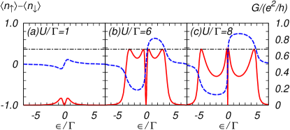
Figure 2: (Color online) The relation between the conductance $G$ (red solid line) and the population difference $\langle n_{\uparrow}\rangle-\langle n_{\downarrow}\rangle$ (blue dashed line) when the two dot levels are degenerate $\epsilon_{1}=\epsilon_{2}=\epsilon$. In all three panels, $t_{1}^{L}:t_{1}^{R}:t_{2}^{L}:t_{2}^{R}=\sqrt{0.27}:\sqrt{0.33}:\sqrt{0.16}:-\sqrt{0.24}$. The black horizontal dash-dotted line represents $G_{\rm max}\approx 0.68(e^{2}/h)$ predicted by Eq. (17). Here $\Gamma\equiv\pi[(|t_{1}^{L}|^{2}+|t_{2}^{L}|^{2})\rho^{L}+(|t_{1}^{R}|^{2}+|t_{2}^{R}|^{2})\rho^{R}]$, where $\rho^{l}$ is the local density of states at the end of the lead $l$. The curves for $G$ are from Fig. 2 in Ref. Meden06PRL while the curves for $\langle n_{\uparrow}\rangle-\langle n_{\downarrow}\rangle$ are obtained comment-fig2 from Eq. (17). (a) For a small $U$, where the PS (sign change of $\langle n_{\uparrow}\rangle-\langle n_{\downarrow}\rangle$ at $\epsilon=0$) is a weak feature and $|\langle n_{\uparrow}\rangle-\langle n_{\downarrow}\rangle|$ remains below the critical value 1/2, only two conductance peaks appear with the peak centers located at the positions where $|\langle n_{\uparrow}\rangle-\langle n_{\downarrow}\rangle|$ is maximized. (b) For a large $U$, where the PS becomes manifest and $|\langle n_{\uparrow}\rangle-\langle n_{\downarrow}\rangle|$ becomes larger than the critical value 1/2 in certain ranges of $\epsilon$, four conductance peaks appear with the peak centers located at the positions where $|\langle n_{\uparrow}\rangle-\langle n_{\downarrow}\rangle|=1/2$; the two peaks close to $\epsilon=0$ are the CIRs while the other two peaks are the Coulomb blockade peaks. (c) For a still larger $U$, where the PS becomes stronger, the distinction between the CIRs and the Coulomb blockade peaks becomes more evident. Note that $G$ is related to the population difference of the transformed dot states, $\langle n_{\uparrow}\rangle-\langle n_{\downarrow}\rangle$, instead of the population difference of the original dot states, $\langle n_{1}\rangle-\langle n_{2}\rangle$.

It is illustrative to compare Eq. (17) with the corresponding expression for the conventional spin Kondo effect in a QD SpinKondoTh , where spin-up and spin-down scattering states generates two incoherent contributions [$\sin^{2}(\pi\langle n_{\uparrow}\rangle)$ vs. $\sin^{2}(\pi\langle n_{\downarrow}\rangle)]$ to the conductance. Thus in the absence of a magnetic field, where $\langle n_{\uparrow}\rangle=\langle n_{\downarrow}\rangle$, $G$ is proportional to $\sin^{2}(\pi\langle n_{\uparrow}\rangle)+\sin^{2}(\pi\langle n_{\downarrow}\rangle)=2\sin^{2}[\pi(\langle n_{\uparrow}\rangle+\langle n_{\downarrow}\rangle)/2]$. In our system, in contrast, the two pseudospin scattering states $\psi_{\uparrow}$, $\psi_{\downarrow}$ should be coherently superposed to construct scattering states in the original system, which are then used to evaluate $G$. This coherent summation procedure takes into account the interference between the two transport paths in Fig. 1(a), one mediated by $\epsilon_{1}$ and the other by $\epsilon_{2}$. This explains the difference between the two expressions for $G$.

Pseudospin fluctuations.— To examine fluctuations of the QD pseudospin $S_{z}\equiv(n_{\uparrow}-n_{\downarrow})/2$, it is useful to map the Hamiltonian ${\cal H}$ into a $s$-$d$ model by using the Schrieffer-Wolff transformation Hewson93Book . In the large $U$ limit and near the center of the Coulomb valley, one finds Kdiagonalization ,

$${\cal H}_{s-d}={\cal H}_{\rm ex}+{\cal H}_{\rm lead}+{\cal H}_{B},$$ (18)

where ${\cal H}_{\rm ex}=\sum_{kk^{\prime}}[J^{+}S^{+}c^{\dagger}_{k\downarrow}c_{k^{\prime}\uparrow}+J^{-}S^{-}c^{\dagger}_{k\uparrow}c_{k^{\prime}\downarrow}+J^{z}S_{z}(c^{\dagger}_{k\uparrow}c_{k^{\prime}\uparrow}-c^{\dagger}_{k\downarrow}c_{k^{\prime}\downarrow})]$, ${\cal H}_{B}=-S_{z}{\cal B}_{z}^{\rm eff}$, and ${\cal B}_{z}^{\rm eff}=B_{z}-\sum_{kk^{\prime}}J^{z,2}_{kk^{\prime}}(c^{\dagger}_{k\uparrow}c_{k^{\prime}\uparrow}+c^{\dagger}_{k\downarrow}c_{k^{\prime}\downarrow})$. Here $c_{k\sigma}$ is the annihilation operator of the eigenstate with energy $\varepsilon_{k}$ in ${\cal H}_{\rm lead}$. The degeneracy of the dot states is still assumed. Various coefficients are defined as follows; $J^{+}=J^{-}=4V_{\uparrow}V_{\downarrow}/U$, $J^{z}=2(V_{\uparrow}^{2}+V_{\downarrow}^{2})/U$, $B_{z}=(V_{\uparrow}^{2}-V_{\downarrow}^{2})\sum_{k}(U/2-\epsilon+\varepsilon_{k})^{-1}$, and $J^{z,2}_{kk^{\prime}}=(V_{\uparrow}^{2}-V_{\downarrow}^{2})[(U/2+\epsilon-\varepsilon_{k^{\prime}})^{-1}+(U/2-\epsilon+\varepsilon_{k})^{-1}]/2$, where $V_{\sigma}\geq 0$ ($V_{\uparrow}/V_{\downarrow}=\lambda_{\uparrow}/\lambda_{\downarrow}$) denotes the matrix element for the tunneling from the dot state $d_{\sigma}$ to the lead state $c_{k\sigma}$. Note that ${\cal H}_{\rm ex}$ becomes an anisotropic antiferromagnetic ($J^{z}>J^{+}>0$) exchange interaction since $V_{\uparrow}\neq V_{\downarrow}$ in general. A crucial difference from the conventional Kondo effects Hewson93Book arises from the pseudomagnetic field ${\cal B}_{z}^{\rm eff}$, whose expectation value $H_{z}$ with respect to the Fermi sea in the leads becomes comment-pseudo-B

$$H_{z}\equiv\langle{\cal B}_{z}^{\rm eff}\rangle={\Gamma_{\uparrow}-\Gamma_{\downarrow}\over\pi}\ln{U/2+\epsilon\over U/2-\epsilon}\,,$$ (19)

where $\Gamma_{\sigma}\equiv\pi\rho_{0}V_{\sigma}^{2}$ and $\rho_{0}$ is the density of states in the leads. Note that $H_{z}$ does depend on $\epsilon$ and changes its sign at $\epsilon=0$, implying the sign change of $\langle S_{z}\rangle=(\langle n_{\uparrow}\rangle-\langle n_{\downarrow}\rangle)/2$ at $\epsilon=0$. This provides a simple explanation of the PS Silvestrov00PRL ; Sindel05PRB ; Kim06PRB . By the way, for the special $t_{j}^{l}$’s discussed in Refs. Boese01PRB ; Meden06PRL , where the conserved pseudospin exists but $\lambda_{\uparrow}=\lambda_{\downarrow}$, $H_{z}$ vanishes since $\Gamma_{\uparrow}=\Gamma_{\downarrow}$.

Next we perform the two-stage poor man’s scaling Hewson93Book , the first stage with the original Hamiltonian ${\cal H}$ and the second stage with ${\cal H}_{s-d}$ up to the second order in $J^{z}$ and $J^{\pm}$. One finds that the $S_{z}$ fluctuations are characterized by the Kondo temperature $T_{K}$ TK-comment ,

$$T_{K}\sim U\exp\left(-{1\over 4\rho_{0}J_{0}}\ln{J^{z}+J_{0}\over J^{z}-J_{0}}\right),$$ (20)

where $J_{0}\equiv\sqrt{(J^{z})^{2}-(J^{+})^{2}}$. Equation (20) may be expressed as $T_{K}\sim U\exp[-\pi U\ln(\Gamma_{\uparrow}/\Gamma_{\downarrow})/8(\Gamma_{\uparrow}-\Gamma_{\downarrow})]$. Interestingly ${\cal B}_{z}^{\rm eff}$ at each step of the scaling shares the same expectation value $H_{z}$ [Eq. (19)].

Figure 3: (a) $\langle S_{z}\rangle=(\langle n_{\uparrow}\rangle-\langle n_{\downarrow}\rangle)/2$ as a function of $H_{z}/T_{K}$ predicted by the exact solution of the anisotropic $s$-$d$ model Tsvelick83AP . $\langle S_{z}\rangle$ for negative $H_{z}$ can be obtained by using $\langle S_{z}\rangle$ being an odd function of $H_{z}$. (b) $G/G_{\rm max}$ vs. $\epsilon/T_{K}$ TK-comment obtained by Eqs. (17), (19), and the $\langle S_{z}\rangle$ vs. $H_{z}$ relation in (a). In these plots, $t_{1}^{L}:t_{1}^{R}:t_{2}^{L}:t_{2}^{R}=\sqrt{0.27}:\sqrt{0.33}:\sqrt{0.16}:-\sqrt{0.24}$ ($\lambda_{\uparrow}/\lambda_{\downarrow}\approx 1.29$), and $U/(\Gamma_{\uparrow}+\Gamma_{\downarrow})=7$ are used. $G/G_{\rm max}$ for negative $\epsilon$ can be obtained by using $G$ being an even function of $\epsilon$. In the inset, the logarithmic scale is used for the horizontal axis.

For further study, we approximate ${\cal H}_{s-d}$ by replacing ${\cal B}_{z}^{\rm eff}$ with $H_{z}$. Properties of the resulting Hamiltonian are well known via the Bethe ansatz method Tsvelick83AP . Figure 3(a) shows the $H_{z}$-dependence of $\langle S_{z}\rangle$ predicted by the exact solution Tsvelick83AP , and Fig. 3(b) shows the resulting $\epsilon$-dependence of $G/G_{\rm max}$ obtained from Eq. (17). For $|H_{z}|\lesssim T_{K}$, $\langle S_{z}\rangle$ is approximately given by $H_{z}/(2\pi T_{K})$ Tsvelick83AP . Within this linear approximation, the CIR peak positions $\epsilon_{\rm CIR}$ are given by

$$\epsilon_{\rm CIR}\approx\pm{U\over 2}\tanh\left({\pi^{2}\over 2}{T_{K}\over\Gamma_{\uparrow}-\Gamma_{\downarrow}}\right).$$ (21)

For $H_{z}\gg T_{K}$, $1/2-\langle S_{z}\rangle$ is proportional to $(T_{K}/H_{z})^{2\mu/\pi}$ Tsvelick83AP , where $\mu\equiv\cos^{-1}[\cos(2\pi\rho_{0}J^{z})/\cos(2\pi\rho_{0}J^{+})]\approx 2\pi\rho_{0}J_{0}$ in the weak tunneling regime $\rho_{0}J^{z}$, $\rho_{0}J^{+}\ll 1$. Due to the small exponent $2\mu/\pi\approx 4\rho_{0}J_{0}\ll 1$, $\langle S_{z}\rangle$ approaches its saturated value $1/2$ very slowly. Combined with Eqs. (17) and (21), this explains the origin of the strongly asymmetric peak shape of the CIRs Meden06PRL .

Discussion.— First we address the case of the nondegenerate dot levels $\epsilon_{1(2)}=\epsilon\pm\delta/2$. For small $\delta$, the two perturbations ${\cal H}_{\rm dot}^{(2)}$, ${\cal H}_{\rm dot}^{(3)}$ due to the nondegeneracy may be treated separately. Effects of ${\cal H}_{\rm dot}^{(2)}$ are rather trivial; After the Schrieffer-Wolff transformation, ${\cal H}_{\rm dot}^{(2)}$ becomes $-S_{z}H_{z}^{\delta}$, which renormalizes $H_{z}$ in Eq. (19) and induces a shift of the CIR peaks to the new positions $\epsilon_{\rm CIR}\approx\pm(U/2)\tanh[\pi^{2}(T_{K}\mp 2H_{z}^{\delta}/\pi)/2(\Gamma_{\uparrow}-\Gamma_{\downarrow})]$. ${\cal H}_{\rm dot}^{(2)}$ does not alter the peak heights. Effects of ${\cal H}_{\rm dot}^{(3)}$ are rather complicated since it breaks the pseudospin conservation. Equation (17) based on the pseudospin conservation is not applicable and we derive below a more general conductance formula. The time-reversal symmetry is assumed for simplicity. Electrons in the transformed lead [Fig. 1(b)] can be described by the following scattering matrix,

$$\left(\begin{array}[]{cc}r_{\uparrow\uparrow}&\tau_{\uparrow\downarrow}\\ \tau_{\downarrow\uparrow}&r_{\downarrow\downarrow}\end{array}\right)=e^{2i\theta_{\rm tot}}\left(\begin{array}[]{cc}e^{2i\theta}\cos\phi&i\sin\phi\\ i\sin\phi&e^{-2i\theta}\cos\phi\end{array}\right),$$ (22)

where $\theta_{\rm tot}=\pi(\langle n_{\uparrow}\rangle+\langle n_{\downarrow}\rangle)/2=\pi/2$ in the Coulomb valley due to the Friedel sum rule Langer61PR . After a similar algebra as in the derivation of Eq. (17), one obtains

$$G=G_{\rm max}|\sin 2\theta\cos\phi-\cot 2\nu\sin\phi|^{2},$$ (23)

where $\nu$ is independent of $\epsilon$ with $\cot^{2}2\nu=(|t_{1}^{L}|^{2}+|t_{2}^{L}|^{2}-|t_{1}^{R}|^{2}-|t_{2}^{R}|^{2})^{2}/4|t_{1}^{L}{t_{1}^{R}}^{*}+t_{2}^{L}{t_{2}^{R}}^{*}|^{2}$ while $\theta$ and $\phi$ in general depend on $\epsilon$. For small $\delta$, the $\epsilon$-dependence of $\theta$ and $\phi$ can be estimated from the knowledge in the limit $\delta\rightarrow 0$, where the pseudospin flip amplitudes $\tau_{\uparrow\downarrow}=\tau_{\downarrow\uparrow}$ approach zero and thus $\phi$ and $\theta$ approach respectively to zero and $\pi(\langle n_{\uparrow}\rangle-\langle n_{\downarrow}\rangle)/2$. Then in generic situations, where $\tau_{\uparrow\downarrow}=\tau_{\downarrow\uparrow}$ do not vanish in the narrow range of $\epsilon$ near the two CIRs, the second term in Eq. (23) does not change its sign near the CIRs whereas the first term changes its sign due to the sign reversal of $\sin 2\theta$. This implies that while the interference between the two terms is destructive near one CIR peak, suppressing the peak height, it is constructive near the other CIR peak, enhancing the peak height. This explains the $\delta$-induced difference of the two CIR peak heights reported in Ref. Meden06PRL .

Next we remark briefly on the conductance at the dip, $G_{\rm dip}$, between the two CIR peaks. For $\delta=0$, the PS always results in $G_{\rm dip}=0$ [Eq. (17)]. For nonzero but small $\delta$, $G_{\rm dip}$ should be still exactly $0$ if the system has the time-reversal symmetry since the exact cancellation of the two terms in Eq. (23) is possible. If the time-reversal symmetry is broken, a further generalization of Eq. (23) indicates that such an exact cancellation is not generic and $G_{\rm dip}$ acquires a finite value. This result is consistent with Ref. Lee99PRL ; Silvestrov03PRL .

In summary, we have demonstrated that a spinless quantum dot system with two degenerate single-particle levels allows a conserved pseudospin and that in the presence of the correlation caused by the strong Coulomb interaction, the fluctuations of the pseudospin at the quantum dot give rise to a pair of asymmetric conductance peaks in a Coulomb valley. The relation between these correlation-induced resonances and the phenomenon of the population switching has been established.

This work was supported by the SRC/ERC program (R11-2000-071) and the Basis Research Program (R01-2005-000-10352-0) of MOST/KOSEF, by the POSTECH Core Research Program, and by the KRF Grant (KRF-2005-070-C00055) funded by MOEHRD.

Note added.— After the submission of our paper, preprints Silvestrov06cond-mat ; Kashcheyevs06cond-mat reporting similar results appeared.

References

• (1) Mesoscopic Electron Transport, edited by L. L. Sohn, L. P. Kouwenhoven, and G. Schön (Kluwer, Dodrecht, 1997).
• (2) M. A. Kastner, Phys. Today 46, 24 (1993).
• (3) T. K. Ng and P. A. Lee, Phys. Rev. Lett. 61, 1768 (1988); L. Glazman and M. Raikh, JETP Lett. 47, 452 (1988).
• (4) D. Goldhaber-Gordon et al., Nature (London) 391, 156 (1998); S. M. Cronenwett et al., Science 281, 540 (1998); W. G. van der Wiel et al., Science 289, 2105 (2000).
• (5) K. A. Matveev, Zh. E’ksp. Teor. Fiz. 98, 1598 (1990) [Sov. Phys. JETP 72, 892 (1991)]; Phys. Rev. B 51, 1743 (1995).
• (6) D. Boese, W. Hofstetter, and H. Schoeller, Phys. Rev. B 64, 125309 (2001).
• (7) U. Wilhelm and J. Weis, Physica E 6, 668 (2000); A. W. Holleitner et al., Phys. Rev. B 70, 075204 (2004).
• (8) E. Schuster et al., Nature (London) 385, 417 (1997).
• (9) P. G. Silvestrov and Y. Imry, Phys. Rev. Lett. 85, 2565 (2000); Phys. Rev. B 65, 035309 (2002).
• (10) J. König and Y. Gefen, Phys. Rev. B 71, 201308(R) (2005); M. Sindel et al., Phys. Rev. B 72, 125316 (2005); M. Goldstein and R. Berkovits, cond-mat/0610810.
• (11) S. Kim and H.-W. Lee, Phys. Rev. B 73, 205319 (2006).
• (12) V. Meden and F. Marquardt, Phys. Rev. Lett. 96, 146801 (2006); C. Karrasch, T. Enss, and V. Meden, Phys. Rev. B 73, 235337 (2006); A spinless parallel double QD system studied in these reports is equivalent to a single QD system with two single-particle levels.
• (13) J. S. Langer and V. Ambegaokar, Phys. Rev. 121, 1090 (1961).
• (14) H.-W. Lee, Phys. Rev. Lett. 82, 2358 (1999).
• (15) Since the mapping from $G$ to $\langle n_{\uparrow}\rangle-\langle n_{\downarrow}\rangle$ in Eq. (17) is multi-valued, we impose the following constraints to resolve the ambiguity; (i) both $\langle n_{\uparrow}\rangle$ and $\langle n_{\downarrow}\rangle$ approach 0 as $\epsilon\rightarrow+\infty$ and 1 as $\epsilon\rightarrow-\infty$, (ii) $\langle n_{\uparrow}\rangle-\langle n_{\downarrow}\rangle$ is positive for $\epsilon>0$ and negative for $\epsilon<0$ (due to the PS mechanism in Ref. Silvestrov00PRL ), (iii) $d(\langle n_{\uparrow}\rangle-\langle n_{\downarrow}\rangle)/d\epsilon$ is a continuous function of $\epsilon$, (iv) near the conductance peaks, $G-G_{\rm max}\propto(\epsilon-\epsilon_{\rm peak})^{2}$, where $\epsilon_{\rm peak}$ denotes the peak center position.
• (16) A. C. Hewson, The Kondo Problem to Heavy Fermions (Cambridge University Press, New York, 1993).
• (17) In addition to the terms in Eq. (18), the Schrieffer-Wolff transformation also generates a potential scattering term. This term is not essential and thus ignored.
• (18) A similar expression appears in the context of a QD coupled to ferromagnetic leads [J. Martinek et al., Phys. Rev. B 72, 121302(R) (2005)]. However its effect on the conductance is considerably different.
• (19) The prefactor of $T_{K}$ in Eq. (20) is not certain. For example, higher order poor man’s scaling may modify the prefactor. In Fig. 3(b), the prefactor is assumed to be exactly $U$ for definiteness of the illustration.
• (20) A. M. Tsvelick and P. B. Wiegmann, Adv. Phys. 32, 453 (1983); In this paper, the low $H_{z}$ series expansion [Eq. (5.2.24)] and the high $H_{z}$ asymptotics [Eq. (5.2.25)] for $\langle S_{z}\rangle$ have some typos while the general formula [Eq. (5.2.20)] is correct.
• (21) H.-W. Lee and C. S. Kim, Phys. Rev. B 63, 075306 (2001); P. G. Silvestrov and Y. Imry, Phys. Rev. Lett. 90, 106602 (2003).
• (22) P. G. Silvestrov and Y. Imry, cond-mat/0609355.
• (23) V. Kashcheyevs et al., cond-mat/0610194.