Orbital Dependence of Quasiparticle Lifetimes in $Sr_{2}RuO_{4}$

Abstract

Using a phenomenological Hamiltonian, we investigate the quasiparticle lifetimes and dispersions in the three low energy bands, $\gamma$, $\beta$, and $\alpha$ of $Sr_{2}RuO_{4}$. Couplings in the Hamiltonian are fixed so as to produce the mass renormalization as measured in magneto-oscillation experiments. We thus find reasonable agreement in all bands between our computed lifetimes and those measured in ARPES experiments by Kidd et al. kidd and Ingle et al. ingle . In comparing computed to measured quasiparticle dispersions, we however find good agreement in the $\alpha$-band alone.

I Introduction

The ruthenate $Sr_{2}RuO_{4}$ has been extensively studied for a number of reasons, chief among them its unconventional superconducting state mack . Its electronic structure, reviewed in detail by Bergemann et al. bergemann , has also been of much interest. Three bands belonging to the $t_{2g}$ complex of 4d $Ru$ orbitals cross the Fermi energy. They are divided into two sets. One derived from the $d_{xy}$ orbital has a two-dimensional dispersion with little dispersion along the c-axis due to the layered structure of the material. The second set comprises the $d_{xz}$ and $d_{yz}$ bands which have predominantly one-dimensional dispersion. A key feature is the absence of hybridization between these sets in a single layer due to the opposite parity under reflection about a $RuO_{2}$ plane. This contrast in their dispersion has been invoked by Kidd and collaborators kidd to explain the strong difference in the energy and temperature dependence of the quasiparticle lifetimes between the two sets observed in recent ARPES (Angle Resolved Photoemission Spectroscopy) experiments. In this note we report on some simple calculations to examine this interpretation.

Figure 1: A schematic of the three bands on $Sr_{2}RuO_{4}$.

The Fermi surface is illustrated in Fig. 1 and consists of three sheets. The almost circular $\gamma$-sheet derives from orbitals with $d_{xy}$ symmetry. The $\alpha$ and $\beta$ sheets derive from the approximately linear sections due to the orbitals with $d_{xz}$ and $d_{yz}$ symmetry which however hybridize weakly with each other where they cross. Kidd and collaborators kidd measured the dispersion and linewidths of the quasiparticles on the $\gamma$- and the $\beta$- sheets along the line $\Gamma$-M and found a clear difference in their behavior as a function of both energy and temperature. Ingle et al. ingle measured the same quantities for the $\alpha$-band along the $\Gamma$-X direction finding similar linewidths to those observed by Kidd et al. in the $\beta$-band. At first sight this difference between the $\gamma$-band and the $\alpha$-, $\beta$-bands would seem to be simply a consequence of their differing dispersion and the lack of hybridization between them. While direct scattering of a quasiparticle between these bands is forbidden due to their different parities, quasiparticles in these band will still interact through the Coulomb interactions which leads to modifications of their strictly one and two-dimensional character. To explore this effect we undertake low order calculations of the lifetime using phenomenological interaction strengths. These interaction strengths are chosen so that the mass renormalization observed in magneto-oscillation experiments mack ; bergemann is reproduced.

Doing so we are able to account for the broad features of the observed linewidths. In particular we obtain a good fit to the linewidths in the $\gamma-$band as a function of binding energy and we find, consistent with experiment that the linewidths in the $\beta$- and $\alpha$-bands are far smaller. Our computations do however consistently underestimate to a small degree the linewidths. This points to, perhaps, some other contributory mechanism beyond electron-electron interactions. We also explored the finite temperature behavior of the linewidths. In both the $\gamma$- and $\beta$- bands, our computations match well the observed behaviour seen in kidd . Unlike the linewidths, the agreement between the measured and computed dispersion relations is mixed. For the $\alpha$-band, good agreement is found while for the $\beta$ and $\gamma$-bands, the measured mass renormalization is far less than what would be expected from magneto-oscillation experiments. We comment on this further in the discussion and conclusion section.

Figure 2: Diagrams contributing to the self energy at first and second order. Here the greek indices $\alpha,\beta$ refer to generic bands.

II Calculations of the Lifetime and Effective Mass

The multi-band Hamiltonian that describes a single layer is as follows

$${\cal H} = {\cal H}_{0}+{\cal H}_{\rm int};$$ (1)

$${\cal H}_{0} = \sum_{k\sigma\mu}\epsilon^{\mu}(k)c^{\dagger}_{\mu k\sigma}c_{\mu k\sigma};$$ (2)

$${\cal H}_{\rm int} = \sum_{\mu,\nu,\sigma,\sigma^{\prime},i}V_{\mu\nu}n_{\mu\sigma}(i)n_{\nu\sigma^{\prime}}(i).$$ (3)

Here the greek indices, $\mu,\nu$, are band indices and sum over the three bands, $\alpha,\beta,$ and $\gamma$. The two-dimensional $\gamma$-band, describing orbitals with $d_{xy}$ symmetry, takes the form morr ; ll ,

$$\epsilon^{\gamma}({\bf k})=-.88\cos(k_{x})-.88\cos(k_{y})-.56\cos(k_{x})\cos(k_{y})-.5.$$ (4)

The one-dimensional $\alpha$- and $\beta$-bands arise from weak hybridization between the $d_{xz}$ and $d_{yz}$ symmetry orbitals and appear as

$$\epsilon^{xz}({\bf k}) = -.62\cos(ak_{x})-.09\cos(ak_{y})$$ (6)

$$\hskip 36.135pt+.04\cos(ak_{x})\cos(ak_{y})-.24;$$

$$\epsilon^{yz}({\bf k}) = -.09\cos(ak_{x})-.62\cos(ak_{y})$$ (8)

$$\hskip 36.135pt+.04\cos(ak_{x})\cos(ak_{y})-.24;$$

$$\epsilon^{\pm}({\bf k}) = \frac{1}{2}(\epsilon^{xz}\pm\epsilon^{yz});$$ (9)

$$\epsilon^{\alpha/\beta} = \epsilon^{+}\mp\sqrt{(\epsilon^{-})^{2}+.01}.$$ (10)

All energies are in eV’s and $a=3.86A^{o}$ is the lattice spacing. The interaction vertices reduce to four terms describing intraband scattering between electrons in the $\gamma$-band ($V_{\gamma\gamma}$) and in the $\alpha$,$\beta$-bands ($V_{\alpha\alpha}=V_{\beta\beta}$) and interband scattering between $\gamma$ and the $\alpha,\beta$-bands($V_{\gamma\alpha}=V_{\gamma\beta}$) and between the $\alpha$ and $\beta$ bands ($V_{\alpha\beta}$). Simple estimates of the Fermi-Thomas screening length give strong screening due to the large density of states at the Fermi energy so we neglect the wavevector dependence of the interaction vertices. This leads to four independent parameters which we adjust phenomenologically as discussed below. The calculation of the self energy is restricted to the lowest orders in the phenomenological interaction vertices, illustrated in Fig 2. For the lifetime this amounts to calculating the decay processes of a single quasihole into three quasiparticles with renormalized interaction vertices. These processes will dominate the decay rate of low energy quasiholes as multiquasiparticle decays will rise more slowly with the energy of the quasihole measured from the Fermi energy. Our aim is to explore the effects of the differing band dispersions on the decay rates.

Our approach to this problem is then in the spirit of Landau Fermi liquid theory – we use the necessary mass renormalization to fit the coupling constants (akin to the Fermi liquid parameters) and then determine other quantities (the inverse lifetimes) in terms of these same couplings. In this spirit, the largeness of certain parameters (for example. the dimensionless coupling $u_{\gamma\gamma}=K_{F\gamma}V_{\gamma\gamma}/2\pi v_{F\gamma}$), should not be taken as problematic.

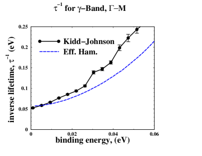
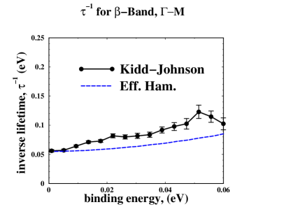
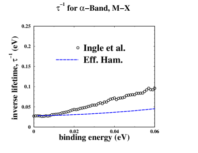
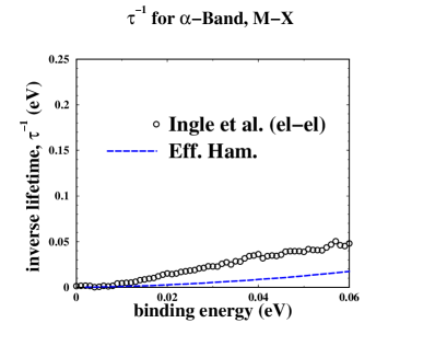
Figure 3: Plots of the inverse lifetimes in the three bands, $\gamma$, $\beta$ and $\alpha$.

The real part of the self energy is calculated employing the same set of diagrams. Any non-zero contribution to the real part at $\omega=0$ at the Fermi surface is absorbed into a redefinition of the chemical potential. The first order diagram, marking the exchange energy, contributes to the real part of the self-energy alone. It is the first in a series of diagrams but is the only member of the series to make a contribution. The remaining diagrams in the series simply renormalize the chemical potential and so are ignored.

	$\alpha$	$\beta$	$\gamma$
dHvA ($m_{*}$)	3.3	7.0	16
ARPES	3.3	2.3	3.0
LDA AV ($m_{LDA})$	1.2	2.3	2.3
$m_{R}=m_{*}/m_{LDA}$	2.8	3.0	7.0

Table 1: Mass renormalization of the electrons in the three bands of $Sr_{2}RuO_{4}$ as given by magneto-oscillation experiments mack ; bergemann (dHvA), ARPES measurements kidd ; ingle , and LDA computations . These three mass renormalizations are all given in terms of the bare electron mass.

To compute the strengths of phenomenological interaction parameters we insist that the computed self energy reproduce the mass renormalizations expected from magneto-oscillation experiments mack ; bergemann (see top line of Table 1). The mass renormalizations induced by the interaction terms in Eq. 2.1 are given by

$$m_{R}=\frac{m_{*}}{m_{LDA}}=\frac{1-\partial_{\omega}{\rm Re}\Sigma(w,k=K_{F})}{1+v_{LDA}^{-1}\partial_{k}{\rm Re}\Sigma(w,k=K_{F})}$$ (11)

where $m_{LDA}$ is the mass renormalization induced by the LDA band structure (also listed in Table I). The LDA values given in Table I are averages around the bands’ Fermi surfaces weighted by the local density of states (appropriate as the magneto-oscillations masses are themselves weighted averages). The interaction strengths are then determined by insisting that $m_{R}$ equal $m_{*}/m_{LDA}$ (as listed in Table 1) at a single point along the Fermi surface of each band. We do not attempt to average $m_{R}$ itself around the Fermi surfaces (requiring a computation of the self-energy everywhere) as too computationally costly.

In the presence of contact interactions, the $T=0$ self-energy for a given band $\mu$ at first order consists of a term independent of both momentum and energy and so may be ignored (at finite $T$, this term however does do more than renormalize the Fermi energy). At second order the contribution takes the form

$$\Sigma_{\mu}(\omega,k) = \sum_{\nu}\Sigma_{\mu\nu}(\omega,k)$$ (12)

$$= \sum_{\nu}\frac{V_{\mu\nu}^{2}}{4\pi^{3}}\int dq\int dx\frac{{\rm Im}\chi_{\nu}(q,x)}{w+i\delta-\epsilon_{\mu}(k-q)-x}$$ (16)

$$\times(\theta(-x)-\theta(\epsilon_{\mu}(k-q))),$$

where $\chi_{\nu}$ is the susceptibility of electrons in band $\nu$. We numerically compute the derivatives of the real part of the self energy necessary to computing $m_{R}$ in order to accurately capture the effect of the dispersion in each of the bands (without recourse to approximating the bands through a quadratic dispersion relation).

The values of the interaction parameters so determined are given in Table II. The first number marks the value used in later computations of the dispersion and lifetime. The ranges in brackets mark the range of parameters producing the desired mass renormalization, $m_{R}$. However other choices within the given ranges yield results for the lifetimes that differ by no more than $10\%$.

$V_{\gamma\gamma}$	$V_{\gamma\beta}$	$V_{\alpha\beta}$	$V_{\beta\beta}$
5.9 (5.1-6.5)	1.4 (0-2)	1.3 (.8-1.6)	1.5 (0-2.1)

Table 2: Strengths of the interaction couplings (all values in $a^{2}\cdot eV$ where $a$ is the lattice spacing.

The largest coupling by far is $V_{\gamma\gamma}$, dictated by the need to produce a mass renormalization of $m_{R}\sim 7$.

The real part of the self-energy will have terms beyond linear order in $\omega$ that however are not necessarily negligible a priori. In three dimensions the real part of the self energy would be expected to take the form

$${\rm Re}\Sigma(\omega)=a\omega+b\omega^{3}+\cdots.$$ (17)

By dimensional analysis $b$ would of the form, ${\rm dimensionless~{}constant}\times E_{F}^{-2}$, and so for $\omega$ small, the cubic term can be ignored. But in two dimensions, the self-energy develops non-analyticities and will appear as

$${\rm Re}\Sigma(\omega)=a\omega+b\omega^{2}{\rm sgn}(\omega)+\cdots.$$ (18)

It thus cannot be immediately neglected.

We can estimate this non-analytic term more precisely. Using chubukov , we know the non-analytic contribution to the self-energy at second order at arbitrary $\omega$ and $k$ is given for bands with quadratic dispersions chu1 by

$${\rm Re}\Sigma^{\rm non-anal.}_{\mu\mu}(\omega,k) = \frac{V^{2}_{\mu\mu}m^{2}_{\mu}}{64\pi^{2}E_{F\mu}}\times$$ (23)

$$\hskip-72.26999pt\bigg{[}(\omega^{2}+\frac{1}{4}(\omega-\epsilon_{\mu}(k))^{2}){\rm sign}(\omega-\epsilon_{\mu}(k))$$

$$\hskip-72.26999pt+(\omega^{2}-\frac{1}{4}(\omega-\epsilon_{\mu}(k))^{2}){\rm sign}(\omega+\epsilon_{\mu}(k))$$

$$\hskip-72.26999pt+\omega^{2}{\rm sign}(\omega)+\omega^{2}{\rm sign}(\frac{\omega}{\epsilon_{\mu}(k)});$$

$$\hskip-72.26999pt-(\omega+\epsilon_{\mu}(k))^{2}{\rm sign}(\frac{\omega+\epsilon_{\mu}(k)}{\epsilon_{\mu}(k)})\bigg{]};$$

$${\rm Re}\Sigma^{\rm non-anal.}_{\mu\neq\nu}(\omega,k) = \frac{V^{2}_{\mu\nu}m_{\mu}m_{\nu}^{2}}{32\pi^{2}K_{F\mu}K_{F\nu}}\times$$ (27)

$$\hskip-72.26999pt\bigg{[}(\omega^{2}+\frac{1}{4}(\omega-\epsilon_{\mu}(k))^{2}){\rm sign}(\omega-\epsilon_{\mu}(k))$$

$$\hskip-72.26999pt+(\omega^{2}-\frac{1}{4}(\omega-\epsilon_{\mu}(k))^{2}){\rm sign}(\omega+\epsilon_{\mu}(k))\bigg{]},$$

where $E_{F\mu}$ is the effective bandwidth of band $\mu$, and $m_{\mu}=K^{2}_{F\mu}/2E_{F\mu}$ with $K_{F\mu}$ the band’s corresponding Fermi wavevector. $\Sigma^{\rm non-anal.}_{\mu\mu}(\omega,k)$ has two contributions: one arising from the non-analyticity in the electron polarizability, $\chi_{\mu}(\omega,q)$, at $q$ near 0 and one from another non-analyticity in $q$ near $2K_{F\mu}$ chubukov . In contrast, the interband contribution to the self energy, $\Sigma_{\mu\nu}$, only sees a non-analytic contribution from $\chi_{\nu}(\omega,q\sim 0)$. To estimate the contribution these terms make to the self-energy we need to estimate the appropriate values for the effective (quadratic) masses appearing in the above. To do so we write down the corresponding expressions for the imaginary part of the self energy:

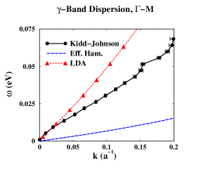
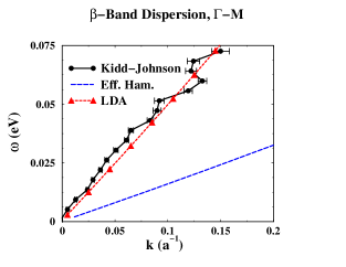
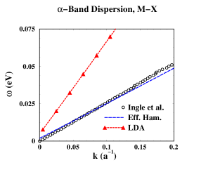
Figure 4: Plots of the dispersion in the three bands, $\gamma$, $\beta$ and $\alpha$.

$${\rm Im}\Sigma_{\mu\mu}(\omega,k) = \frac{V^{2}_{\mu\mu}m^{2}_{\mu}}{32\pi^{3}E_{\mu}}\times$$ (33)

$$\hskip-86.72377pt\bigg{[}(\omega^{2}+\frac{1}{4}(\omega-\epsilon_{\mu}(k))^{2})\ln(\big{|}\frac{\omega-\epsilon_{\mu}(k)}{E_{F\mu}}\big{|})$$

$$\hskip-86.72377pt+(\omega^{2}-\frac{1}{4}(\omega-\epsilon_{\mu}(k))^{2})\ln(\big{|}\frac{\omega+\epsilon_{\mu}(k)}{E_{F\mu}}\big{|})$$

$$\hskip-86.72377pt-\omega^{2}+\frac{\omega\epsilon_{\mu}(k)}{2}$$

$$\hskip-86.72377pt+\omega^{2}\ln(\big{|}\frac{\omega}{E_{F\mu}}\big{|})+\omega^{2}\ln(\big{|}\frac{\omega}{\epsilon_{\mu}(k)}\big{|});$$

$$\hskip-86.72377pt-(\omega+\epsilon_{\mu}(k))^{2}\ln(\big{|}\frac{\omega+\epsilon_{\mu}(k)}{\epsilon_{\mu}(k)}\big{|})\bigg{]};$$

$${\rm Im}\Sigma_{\mu\neq\nu}(\omega,k) = \frac{V^{2}_{\mu\nu}m_{\mu}m_{\nu}^{2}}{16\pi^{3}K_{F\mu}K_{F\nu}}\times$$ (38)

$$\hskip-86.72377pt\bigg{[}(\omega^{2}+\frac{1}{4}(\omega-\epsilon_{\mu}(k))^{2})\ln(\big{|}\frac{\omega-\epsilon_{\mu}(k)}{E_{F\mu}}\big{|})$$

$$\hskip-86.72377pt+(\omega^{2}-\frac{1}{4}(\omega-\epsilon_{\mu}(k))^{2})\ln(\big{|}\frac{\omega+\epsilon_{\mu}(k)}{E_{F\mu}}\big{|})$$

$$\hskip-86.72377pt-\omega^{2}+\frac{\omega\epsilon_{\mu}(k)}{2}\bigg{]}.$$

To determine $E_{F\mu}$, we fit a numerical evaluation of the imaginary part of self-energy via Eqn. 2.5 to the above expression. (The non-analytic portion of ${\rm Im}\Sigma(\omega,k)$ dominates because of the presence of the logs.) Having so extracted effective Fermi energies, $E_{F\mu}$ (see Table III), we then are able to evaluate the non-analytic real part of the self-energy. We find that it makes a significant contribution only for $\omega>.04eV$ and then only for ${\rm Re}\Sigma_{\gamma\gamma}$ – the dispersion relations for the $\alpha$ and $\beta$-bands are insensitive to this correction.

$E_{F\gamma}$	$E_{F\beta}$	$E_{F\alpha}$
0.6	0.5	1.

Table 3: The effective bandwidths for each of the three bands.

While the spirit of our computation is Landau Fermi liquid theory, we can nonetheless address the question of what contribution higher order diagrams (beyond those in Figure 2) make to the inverse lifetime. This is a difficult question of course, but for at least an infinite subset of diagrams studied by Chubukov et al. chubukov , we can give a definitive answer: not much. We focus on $\Sigma_{\gamma\gamma}$ (i.e. the contribution to the self energy of the $\gamma$-band due to the polarizability of $\gamma$-band electrons) as $V_{\gamma\gamma}$ is the largest coupling. Chubukov et al. chubukov have studied the behaviour of higher order forward scattering terms in the $V_{\gamma\gamma}$-perturbative series. They found that the relevant expansion parameter is $s=u_{\gamma\gamma}^{2}\omega/(\omega-\epsilon_{\gamma}(k))$. In terms of our lifetime computations, we are far off the mass shell because of the large mass renormalizations involved, i.e. $(\omega-\epsilon_{\gamma}(k))/\omega\sim 6$, $s$ will be smaller than might first appear, i.e. $s\sim 4$. While the radius of convergence of the series is unclear, if the series needs to be resummed, the effects are not particularly drastic. The terms in ${\rm Im}\Sigma(\omega,k)$ (see Eqn. 2.8) behaving as $\omega^{2}\ln(\omega)$ are modified to

$$\omega^{2}\ln(\frac{\omega}{E_{F\gamma}})\rightarrow\omega^{2}(\frac{1}{2}\ln(\frac{\omega}{E_{F\gamma}})-\frac{1}{2}|\ln(u^{2})|)$$ (39)

Given that $u_{\gamma\gamma}\sim 5$ and $E_{F\gamma}\sim 0.5eV$, for very small $\omega$ we would then expect higher order contributions to lead to a reduction in the inverse lifetime while for omega larger than $.02eV$, higher order contributions leave the answer effectively unchanged.

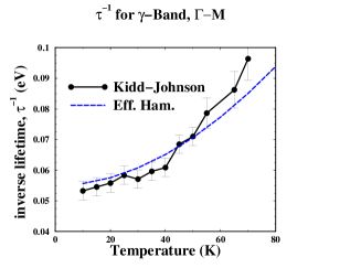
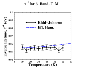
Figure 5: Plots of the temperature dependence in the $\gamma$- and $\beta$-bands..

III Comparison to ARPES Results

The ARPES studies of Kidd and collaborators kidd reported inverse lifetime results for a hole in the $\gamma$ and $\beta$ bands measured along the $\Gamma-M$ direction as a function of energy and of temperature. There is a pronounced difference between the bands with the inverse lifetime for holes in the $\gamma$-band rising much more rapidly with energy and temperature than in the $\beta$-band. The results for the $\beta$-band are mimicked by the linewidths observed in the $\alpha$-band in ingle .

In the top panel of Figure 3, we plot our computed inverse lifetime as a function of binding energy for the $\gamma$ and $\beta$-bands along $\Gamma-M$. To our computed result of the $\gamma$-band, we have added a static impurity contribution of ${\rm Im}\Sigma_{\rm imp}=.055eV$. This is chosen so that the experimental and theoretical values of the inverse lifetime coincide at $\omega=0$. To arrive at the experimental values of the inverse lifetime, we have taken the MDC widths as measured by Kidd et al. and multiplied them by the corresponding LDA value of the band velocity, $v_{F-LDA}$. For the $\gamma$-band this velocity changes rapidly near the Fermi surface and so we have correspondingly employed a $k$-dependent $v_{F-LDA}$. This yields a slightly larger experimental inverse lifetime than reported in kidd . While our computed values undershoot the measured values of the inverse lifetime, the agreement is reasonable for the $\gamma$-band and would be improved significantly if we treated ${\rm Im}\Sigma_{\rm imp}$ as a completely free parameter. In particular, we note that the uncertainties in the measured values do not reflect the uncertainty in the correct value of the bare LDA velocity to employ in converting an MDC width to an inverse lifetime.

For the $\beta$-band the computed and measured values of the inverse lifetime broadly match. In particular, the predicted and measured linewidths are much smaller than in the $\gamma$-band. Again we have added an impurity contribution to the computed inverse lifetime values so that the measured and computed values agree at zero binding energy. We do note however that the computed inverse lifetime is smaller than that measured. Over a range of binding energies of $.06eV$, the measured inverse lifetime increases by $\sim.05eV$ whereas the computed value increases only by half that. This disagreement may be in part explained by the presence at larger energies of correspondingly large error bars. However, unlike for the $\gamma-$ band, the band velocity in the $\beta$-band is not a strong function of wavevector.

In the bottom two panels of Figure 3, we plot our computed lifetime for the $\alpha$-band along the $M-X$ direction vs that measured by Ingle et al. ingle . Ingle et al. use samples with freshly cleaved surfaces where the $\alpha$-band can be resolved without employing surface aging. In the left panel, we plot our computations, again with a correcting ${\rm Im}\Sigma_{\rm imp}$, against the values measured by Ingle et al.. In the right panel we plot our computations (with no impurity correction) against the measured electron-electron contribution to the self-energy. Ingle et al. deduce this contribution by subtracting out an estimate of both the phonon contribution and the impurity contribution. Again we see that the computed value of the inverse lifetime in the $\alpha$-band is much less than that of the $\gamma$-band. However like the $\beta$-band, this value is less than that measured. If we look at only the value imputed to the electron-electron contribution, we see a rise in the inverse lifetime of $.05eV$ over a $.06eV$ range of binding energies whereas our computed value rises by a little less than $.02eV$.

In Figure 4 we compare the corresponding computed and measured dispersion relations for the three bands. The computed dispersions are essentially straight lines whose slope is determined by the value of the dHvA mass renormalizations (as this is how we determine the coupling strength). We have also plotted the LDA dispersion relations. For the $\gamma$- and $\beta$- bands, there is strong disagreement between measured and computed values. Alternatively, the measured dispersion for the $\beta$- and $\gamma$- bands show a mass renormalization far smaller than seen in magneto-oscillation experiments. For the $\beta$-band, the measured mass renormalization equals its LDA prediction. In the $\alpha$-band, in contrast, the dispersion closely matches the computed prediction, that is, the mass renormalization in the $\alpha$-band measured by ARPES closely matches that measured by dHvA.

Finally in Figure 5 we compare the computed temperature dependencies of the inverse lifetimes at zero binding energy in the $\gamma$- and $\beta$-bands to that measured by Kidd et al. kidd . The $\beta$-band results are well-matched. Both computed and measured values show only a weak dependence on temperature over a 100K range. Our computations, nonetheless are consistent with a quadratic Fermi-liquid like dependency on the temperature.

The $\gamma$-band results also agree well with that reported in kidd . We roughly expect the temperature dependency to behave as $A_{T}T^{2}\log(E_{F}/T)$ where $A_{T}$ is some constant. Similarly we expect the dependency of $\tau^{-1}$ on binding energy to be (at leading order, modulo the complications of Eqn. 9) $A_{\omega}\omega^{2}\log(E_{F}/\omega)$. From fits of the two computed curves we find that $A_{T}/A_{w}\sim 10$. The value of this ratio compares well with the expected value, $\pi^{2}$, from a single quadratic band chubukov .

IV Discussion and Conclusions

A primary conclusion from our analysis to the inverse lifetimes and effective masses is that there is a marked difference between the two sets of bands, $\gamma$, and $\alpha$ and $\beta$ in terms of effective coupling strengths. This difference is not a simple consequence of the band dispersion and its effect on the density of states in intraband scattering processes, but rather it is due to a stronger effective intraband interaction in the $\gamma$-band at low energies. This conclusion is rather surprising since all three bands derive from orbitals belonging to the same $t_{2g}$ manifold and standard multiband Hubbard models assign equal onsite interactions to all three orbitals eremin ; millis . Our results point to substantially different renormalizations of the low energy effective intraband interactions in the two sets of bands.

The different standing of the band $\gamma$ from the bands $\alpha$ and $\beta$ may arise from the latter two band’s highly one dimensional character. This character raises the question of whether some form of Luttinger liquid behavior is occurring. The fact that the transport properties show clear three-dimensional Landau-Fermi behavior bergemann shows this behavior dominates at low energy. Nonetheless a crossover to Luttinger liquid behavior could appear at higher energies. However the ARPES data reported by both Kidd et al. kidd and Ingle et al. ingle show no sign of such a crossover up to energies of 60 meV. Both the $\beta$ and $\alpha$ bands appear to have inverse lifetimes that depend quadratically on the binding energy. This perhaps is due to the hybridization and interband scattering between the three bands which act to suppress a strictly one-dimensional character in the $\alpha,\beta$- bands.

Our computed inverse lifetimes broadly match the scale of the observed linewidths in all three bands. Nonetheless they also consistently underestimate the corresponding measured values, more pronouncedly in the $\alpha$- and $\beta$- bands than in the the $\gamma$-band. This might suggest that some additional mechanism is making a contribution to the self energy, at least in the $\alpha$- and $\beta$-bands. This might point to a possible role played by some bosonic mechanism such as phonons. However if the shortfall is to be explained by phonons, phonons need to make a greater contribution to the self energy than posited in Ingle et al. ingle . As we can see from the bottom right panel of Figure 2, the portion of the self-energy in the $\alpha$-band measured by ingle due to electron-electron interactions is double that computed in our effective model.

In the $\gamma$- and $\beta$-bands we see that ARPES predicts a mass renormalization far smaller than that found in magneto-oscillation experiments. This might suggest that there is an effective scale in the problem below the sensitivity of typically ARPES measurements (i.e. $\ll 1meV$). However we also found that the ARPES dispersion in the $\alpha$-band closely matches that predicted by dHvA measurements. This might suggest that the surface aging performed by kidd to distinguish the bulk $\gamma$- and $\beta-$ bands from the surface counterparts changes the mass renormalization in some unexpected fashion. However our match to the $\alpha$-band dispersion measured in ingle is not without difficultly. Our match to their dispersion is predicated solely on electron-electron interactions. If we were to ascribe a role to phonons, it would mean we have overestimated the coupling strengths, $V_{\mu\nu}$. This in turn would mean we have overestimated the inverse lifetimes. But our inverse lifetimes are already smaller than the measured values. It is unclear whether phonons could then self-consistently make up the difference. Nor is it unproblematic to have phonons be the dominant interaction in a material where it is believed electron-electron interactions are responsible for its superconductivity.

Of course, the discrepancies found in regards to the real part of self energy might simply point to a need to go beyond our use of low order diagrams based on an effective Hamiltonian. It would be interesting to attempt a more sophisticated treatment of the set of interacting bands in $Sr_{2}RuO_{4}$. One approach may be to adopt a functional RG approach shankar . Extensive work of this sort has already been done on one-band two dimensional systems honer . It should be possible to extend this work to a multi-band system.

We thank both Peter Johnson and Tim Kidd for numerous useful discussions and direct access to their data. We are also grateful to A. Damascelli for providing us with data from Ref. ingle . RMK acknowledges support from US DOE under contract number DE-AC02 -98 CH 10886. TMR acknowledges hospitality from the Institute for Strongly Correlated and Complex Systems at BNL.

References

- (1) T. E. Kidd, T. Valla, A. V. Fedorov, P. D. Johnson, R. J. Cava and M. K. Haas, Phys. Rev. Lett. 94, 107003, (2005).
- (2) N. J. C. Ingle, K. M. Shen, F. Baumberger, W. Meervasana, D. H. Lu, Z. X. Shen, A. Damascelli, S. Nakatsuji, Z. Q. Mao, Y. Maeno, T. Kimura and Y. Tokura, Phys. Rev. B 72, 205114, (2005).
- (3) A. P. Mackenzie and Y. Maeno, Rev. Mod. Phys. 75 657 (2003).
- (4) C. Bergemann, A. P. Mackenzie, S. Julian, D. Fortsythe and E. Ohmichi, Adv. Phys. 52 639 (2003).
- (5) D. Morr, P. Trautman, and M. Graf, Phys. Rev. Lett. 86 (2001) 5978.
- (6) A. Liebsch and A. Lichtenstein, Phys. Rev. Lett. 84 (2000) 1591.
- (7) I. Eremin, D. Manske and K. H. Bennemann, Phys. Rev. B 65, 220502(R) (2002).
- (8) S. Okamoto and A. Millis, cond-mat/0402267.
- (9) A. Chubukov and D. Maslov, Phys. Rev. B 68, 155113 (2003); A. Chubukov, D. Maslov, S. Gangadharaiah, L. Glazman, Phys. Rev. B 71, 205112 (2005).
- (10) Deviations from a quadratically dispersing band can lead to a change in the non-analytical structure of the self-energy (A. Chubukov and A. Millis, cond-mat/0604496) if the curvature of the band at the Fermi surface in the transverse direction vanishes. This is not the case here.
- (11) R. Shankar, Rev. Mod. Phys. 66, 129 (1994).
- (12) C. Honerkamp, M. Salmhofer, and T. M. Rice, Euro. Phys. J. B 27, 127 (2004), C. Honerkamp, D. Rohe, S. Andergassen, and T. Enss, Phys. Rev. B 70, 235115 (2004).