Nonlinear Seebeck and Peltier Effects in Quantum Point Contacts

Abstract

The charge and entropy currents across a quantum point contact is expanded as a series in powers of the applied bias voltage and the temperature difference. After that, the expansions of the Seebeck voltage in temperature difference and the Peltier heat in current are obtained. With a suitable choice of the average temperature and chemical potential, the lowest order nonlinear term in both cases appear to be of third order. The behavior of the third-order coefficients in both cases are then investigated for different contact parameters.

I INTRODUCTION

Various aspects of the ballistic electron transport across quantum point contacts are studied extensively in the past. The most striking feature of this transport is the quantization of conductanceqc1 ; qc2 at integer multiples of the conductance quantum $2e^{2}/h$. This phenomenon is usually treated with the Landauer-Büttiker formalismlandauer ; buttiker1 which provides a transparent explanation for the effect. Electrons in each sub-band corresponding to the transverse modes in the contact contribute one quantum to the conductance if the sub-band is sufficiently populated. As the size of the constriction is changed by varying the negative voltage on split gates, which are used to define the contact on a two-dimensional electron gas, the conductance changes in smooth steps from one conductance quantum into the other. It is observed that the linear Seebeck and Peltier coefficients for these structures display quantum oscillationsstreda ; proetto ; houten ; molenkamp1 ; molenkamp2 with peaks coincident with the conductance steps.

Nonlinear transport in these systems has also been studied extensively both theoreticallyma:weak ; ma:harm ; ma:kinetic ; qiao ; todorov ; bogachek1 ; bogachek2 and experimentally.krishnaswamy ; dzurak Since Onsager’s reciprocity relations connecting the Seebeck and Peltier transport coefficients loose its meaning in this regime, these two effects show distinctively different behavior. New peaks appear in the differential Peltier coefficient as the driving voltage is increased,bogachek1 ; bogachek2 while the thermopower does not change much even for very large temperature differences.dzurak

A major theoretical difficulty in the nonlinear regime is, due to the small size of these systems, finite voltage differences create large changes in the distribution of electrons around the contact. As a result, more involved calculations are necessary for describing the electron transport.buttiker2 ; christen However, it is of some interest to analyze the nonlinear transport properties without taking such changes into account. The purpose of this article is to investigate the nonlinearities in not so commonly studied Seebeck and Peltier effects, assuming that the contact potential is not changed apart from the uniform shift caused by the gate voltage. It is hoped that this will clarify the importance of the effects mentioned above. In the following section, the charge and heat currents are expanded as a series in powers of the potential and temperature differences. Appropriate expansions for the Seebeck and Peltier phenomena are obtained and the series coefficients are investigated in sections 2 and 3, respectively. Finally, the results are summarized and discussed.

II Theory

In the following we consider two electron gases connected by a quantum point contact. The chemical potentials $\mu_{L}$ and $\mu_{R}$ and the temperatures $\theta_{L}$ and $\theta_{R}$ of the left ($L$) and right ($R$) reservoirs are the parameters that define the whole system. The difference between the chemical potentials, $\Delta\mu=\mu_{L}-\mu_{R}$, is equal to $(-e)V$ where $V$ is interpreted as the electrical potential difference between $L$ and $R$. A difference in temperatures $\Delta\theta=\theta_{L}-\theta_{R}$ as well as a potential difference cause electron transport which can carry both charge and heat across the contact. The average currents on the contact are completely determined by the sum

$$T(E)=\sum_{n}T_{n}(E)\quad,$$

where $T_{n}(E)$ is the transmission probability of an electron with energy $E$ incident from the $n$th mode. The charge and entropy currents from $L$ to $R$ can then be expressed asform:imry

$$I = 2\frac{(-e)}{h}\int_{-\infty}^{\infty}dE(f(x_{L})-f(x_{R}))T(E)\quad,$$ (1)

$$I_{S} = 2\frac{k_{B}}{h}\int_{-\infty}^{\infty}dE(s(x_{L})-s(x_{R}))T(E)\quad,$$ (2)

where

$$f(x) = \frac{1}{1+e^{x}}\quad,$$ (3)

$$s(x) = -f(x)\log f(x)-(1-f(x))\log(1-f(x)),$$ (4)

$$x_{L,R} = \frac{E-\mu_{L,R}}{k_{B}\theta_{L,R}}\quad,$$ (5)

and the spin degeneracy factor is added for both currents.

For the case of weak nonlinearities, it is useful to expand the currents in terms of the driving temperature and potential differences $\Delta\theta$ and $V$. In order to do this the variable of integration is changed from energy $E$ to a dimensionless variable denoted by $\overline{x}$, which is defined as the arithmetic average of $x_{L}$ and $x_{R}$.

$$\overline{x}=\frac{1}{2}(x_{L}+x_{R})\quad.$$

This leads us to define average temperature and chemical potentials by

$$\overline{x} = \frac{E-\overline{\mu}}{k_{B}\overline{\theta}}\quad,$$ (6)

$$\overline{\theta} = \frac{2\theta_{L}\theta_{R}}{\theta_{L}+\theta_{R}}\quad,$$ (7)

$$\overline{\mu} = \frac{\theta_{R}\mu_{L}+\theta_{L}\mu_{R}}{\theta_{R}+\theta_{L}}\quad.$$ (8)

Here, $\overline{\theta}$ is the harmonic average of the temperatures of the two electron gases and $\overline{\mu}$ is an average of chemical potentials weighted by inverse temperatures. These two quantities will be considered as the fundamental parameters describing the contact. In other words all of the transport coefficients are considered as functions of these average quantities.

With these definitions the energy variable can expressed as $E=\overline{\mu}+\overline{x}k_{B}\overline{\theta}$ and the difference of the dimensionless $x$ parameter is

$$\Delta x=x_{L}-x_{R}=-\frac{\Delta\mu+\overline{x}k_{B}\Delta\theta}{k_{B}\theta_{A}}$$ (9)

where $\theta_{A}$ is the arithmetic average of the temperatures on both sides of the contact

$$\theta_{A}=\frac{1}{2}(\theta_{L}+\theta_{R})\quad.$$

Finally, dimensionless driving forces are defined as

$$\epsilon = \frac{\Delta\theta}{\theta_{A}}\quad,$$ (10)

$$\delta = \frac{\Delta\mu}{k_{B}\theta_{A}}\quad.$$ (11)

The obvious advantage of these definitions is the elimination of some terms in the power series expansion of the integrands in equations (1) and (2). We have

$$I = 2\frac{(-e)}{h}\sum_{m=0}^{\infty}\frac{k_{B}\overline{\theta}}{2^{2m}(2m+1)!}\times$$ (12)

$$\times \int d\overline{x}~{}(\delta+\overline{x}\epsilon)^{2m+1}f^{(2m+1)}(\overline{x})T(\overline{\mu}+\overline{x}k_{B}\overline{\theta})\quad,$$

$$I_{S} = 2\frac{k_{B}}{h}\sum_{m=0}^{\infty}\frac{k_{B}\overline{\theta}}{2^{2m}(2m+1)!}\times$$ (13)

$$\times \int d\overline{x}~{}(\delta+\overline{x}\epsilon)^{2m+1}s^{(2m+1)}(\overline{x})T(\overline{\mu}+\overline{x}k_{B}\overline{\theta})\quad,$$

where even order derivatives of the functions $f(x)$ and $s(x)$ have disappeared. This is the primary reason for defining the averages in Eqs. (7) and (8) in this particular way. Defining the parameters

$$f_{m,p}=f_{m,p}(\overline{\mu},\overline{\theta})=(-1)^{m}\int d\overline{x}~{}\overline{x}^{p}f^{(m)}(\overline{x})T(\overline{\mu}+\overline{x}k_{B}\overline{\theta})\quad,$$ (14)

which are only functions of the contact parameters $\overline{\mu}$ and $\overline{\theta}$, the currents can be expressed as

$$I = 2\frac{(-e)}{h}k_{B}\overline{\theta}\sum_{m=0}^{\infty}\sum_{p=0}^{2m+1}\frac{f_{2m+1,p}\epsilon^{p}\delta^{2m+1-p}}{2^{2m}p!(2m+1-p)!}\quad,$$ (15)

$$I_{S} = 2\frac{k_{B}}{h}k_{B}\overline{\theta}\sum_{m=0}^{\infty}\sum_{p=0}^{2m+1}\frac{[f_{2m+1,p+1}-2mf_{2m,p}]\epsilon^{p}\delta^{2m+1-p}}{2^{2m}p!(2m+1-p)!}\quad.$$ (16)

This is the desired expansion of currents in terms of the driving forces $\epsilon$ and $\delta$ with the coefficients being functions of the average quantities $\overline{\mu}$ and $\overline{\theta}$.

One notable property of the equations (15) and (16) is that only the odd powers of the driving forces combined together appear in those expressions. This implies that if both driving forces change sign $\epsilon\rightarrow-\epsilon$ and $\delta\rightarrow-\delta$ then the charge and entropy currents change direction. Including only up to the third order terms in the expansions we have

$$I = 2\frac{(-e)}{h}k_{B}\overline{\theta}\left(f_{10}\delta+f_{11}\epsilon\right.$$ (17)

$$\left.+\frac{1}{24}\left(f_{30}\delta^{3}+3f_{31}\delta^{2}\epsilon+3f_{32}\delta\epsilon^{2}+f_{33}\epsilon^{3}\right)+\cdots\right)$$

$$I_{S} = 2\frac{k_{B}^{2}\overline{\theta}}{h}\left(f_{11}\delta+f_{12}\epsilon+\frac{1}{24}\left((f_{31}-2f_{20})\delta^{3}+3(f_{32}-2f_{21})\delta^{2}\epsilon\right.\right.$$ (18)

$$\qquad\left.\left.+3(f_{33}-2f_{22})\delta\epsilon^{2}+(f_{34}-2f_{23})\epsilon^{3}\right)+\cdots\right)$$

These equations give the currents for arbitrary values of the temperature and potential differences. However, measurements are rarely carried out for arbitrary $\Delta\theta$ and $V$. Electrical conductance and Peltier effect measurements are carried out at isothermal conditions while the thermal conductance and Seebeck effect measurements are done with zero electrical current. But, the equations above is a starting point for each particular phenomenon. In the following, only the Seebeck and Peltier effects are investigated.

III Seebeck Effect

In the Seebeck effect, a temperature difference creates a potential difference across the point contact when there is no electrical current ($I=0$). This potential difference can be expressed in dimensionless form as

$$-\delta=\sigma_{1}\epsilon+\sigma_{3}\epsilon^{3}+\sigma_{5}\epsilon^{5}+\cdots$$ (19)

where the first two coefficients are

$$\sigma_{1} = \frac{f_{11}}{f_{10}}$$ (20)

$$\sigma_{3} = \frac{1}{24f_{10}}\left(f_{33}-3f_{32}\sigma_{1}+3f_{31}\sigma_{1}^{2}-f_{30}\sigma_{1}^{3}\right)$$ (21)

In terms of $V$ and $\Delta\theta$ the series expansion is

$$-V=S_{1}\Delta\theta+S_{3}\Delta\theta^{3}+S_{5}\Delta\theta^{5}+\cdots$$ (22)

where

$$S_{m}=\frac{k_{B}}{(-e)}\frac{1}{\theta_{A}^{m-1}}\sigma_{m}\qquad m=1,3,5,\ldots$$

Appearance of only the third order terms in Eq. (22) implies that when the temperatures of the two reservoirs are exchanged (in other words the sign of $\Delta\theta$ is changed without changing $\theta_{A}$ and $\overline{\theta}$), the induced potential difference due to the Seebeck effect is reversed.

The nonlinear terms in Eq. (22) becomes significant when

$$\Delta\theta_{\mathrm{threshold}}\sim\sqrt{\left|\frac{S_{1}}{S_{3}}\right|}\quad.$$

It is possible to get a theoretical estimate of this quantity in the small temperature limit, when $k_{B}\overline{\theta}\ll E_{L}$, where $E_{L}$ is the energy range where $T(E)$ changes by one. In this case, the Taylor series expansion

$$T(\overline{\mu}+xk_{B}\overline{\theta})\approx T(\overline{\mu})+xk_{B}\overline{\theta}T^{\prime}(\overline{\mu})$$

in Eq. (14) gives the following approximate expressions for $\sigma_{1}$ and $\sigma_{3}$

$$\sigma_{1}\approx\frac{\pi^{2}}{3}\frac{T^{\prime}}{T}k_{B}\overline{\theta}\quad,\qquad\sigma_{3}\approx\frac{\pi^{2}}{12}\frac{T^{\prime}}{T}k_{B}\overline{\theta}\quad.$$

The threshold level for nonlinearity is then

$$\Delta\theta_{\mathrm{threshold}}\sim 2\theta_{A}=\theta_{L}+\theta_{R}\quad.$$

Since $\Delta\theta$ can never go above this level, the nonlinearities in the Seebeck effect are always small.dzurak For this reason, the expansion (22) is appropriate for almost all nonlinear cases. For the opposite, high temperature limit, numerical calculations of the Seebeck coefficients indicates that the threshold expression given above does not change much.

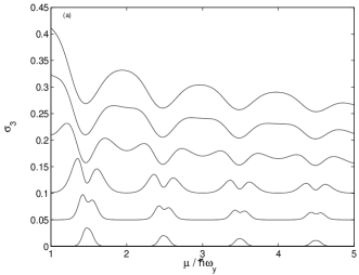
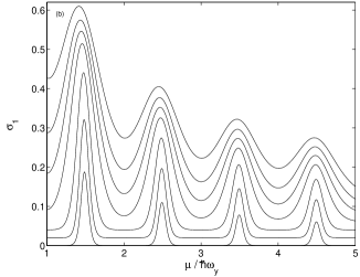
Figure 1: (a) The third order Seebeck coefficient, $\sigma_{3}=(-e)\theta_{A}^{2}/k_{B}~{}S_{3}$, is plotted as a function of average chemical potential $\overline{\mu}$ for $\omega_{y}/\omega_{x}=6$ and $k_{B}\overline{\theta}/\hbar\omega_{y}=$ 0.01, 0.02, 0.04, 0.08, 0.105 and 0.125 (from bottom to top). Each curve is shifted by 0.05 units for clarity. (b)For comparison the linear Seebeck coefficient, $\sigma_{1}=(-e)/k_{B}~{}S_{1}$, is plotted for the same set of parameters. Each curve is shifted by 0.02 units and the temperature increases from bottom to top.

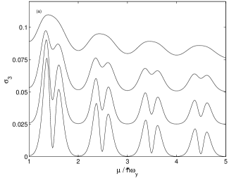
Figure 2: (a) The third order Seebeck coefficient, $\sigma_{3}=(-e)\theta_{A}^{2}/k_{B}~{}S_{3}$, is plotted as a function of average chemical potential $\overline{\mu}$ for $k_{B}\overline{\theta}/\hbar\omega_{y}=0.04$ and $\omega_{y}/\omega_{x}=$ 1.5, 3, 6 and 12 (from top to bottom) respectively. Each plot is shifted by 0.025 units for clarity. (b)For comparison, the linear Seebeck coefficient, $\sigma_{1}=(-e)/k_{B}~{}S_{1}$, is plotted for the same set of parameters. Each plot is shifted by 0.2 units and $\omega_{y}/\omega_{x}$ ratio increases from top to bottom.

As for the general behavior of $S_{3}$, we calculate it for a contact defined by the saddle potential

$$V(x,y)=-\frac{1}{2}m\omega_{x}^{2}x^{2}+\frac{1}{2}m\omega_{y}^{2}y^{2}\quad.$$

For this case the energy dependent transmission probability for the $n$th transverse mode ($n=0,1,2,\ldots$) is

$$T_{n}(E)=\frac{1}{1+\exp\left(-\frac{2\pi}{\hbar\omega_{x}}[E-\hbar\omega_{y}(n+\frac{1}{2})]\right)}\quad.$$

In Fig. 1, $S_{3}$ is plotted against $\overline{\mu}$ for this potential. At sufficiently low temperatures, third order Seebeck coefficient, $S_{3}$, has single peaks coincident with the peaks of $S_{1}$. When the temperature is increased, these peaks start to split into two. This change happens around $k_{B}\overline{\theta}/\hbar\omega_{x}\sim 0.08$. It is observed that the distance between the peaks is proportional to the temperature. For this reason, with increasing temperature, the structure develops into two separate peaks. Also, the widths of the peaks increase proportionally with the temperature. Inevitably, when the temperature is increased further (around $k_{B}\overline{\theta}/\hbar\omega_{y}\sim 0.08$), each peak of the pair starts overlapping with the peaks of the neighboring steps. For this reason, in this high temperature regime the nonlinearity in the Seebeck effect becomes more significant away from the steps (at the plateaus of the electrical conductance). Same graphs are shown in Fig. 2 for different values of $\omega_{y}/\omega_{x}$ ratio. It can be seen that $S_{3}$ has single peaks for small values of $\omega_{y}/\omega_{x}$ ratio (around $\omega_{y}/\omega_{x}\sim 1$), and peak splitting occurs for larger values of the $\omega_{y}/\omega_{x}$ ratio.

In all cases it can be seen that $S_{3}$ is always negative ($\sigma_{3}$ is always positive) and never changes sign. It implies that the nonlinearity increases the generated Seebeck voltage further than the linear term alone suggests. Note that this feature of $S_{3}$ is not apparent from its definition, Eqn. (21). This appears to be a model dependent feature. Especially if $T(E)$ may decrease for some energies, $S_{3}$ may display sign changes. But for the saddle potential model and for all parameter ranges investigated in this study, $S_{3}$ is found to have the same sign.

IV Peltier Effect

The Peltier heat is defined as the heat carried $\dot{Q}=\theta I_{S}$ by the charge current $I$ at isothermal conditions ($\theta_{L}=\theta_{R}=\theta$). The expansion of the Peltier heat and the charge current in terms of the $\delta$ parameter is

$$\dot{Q} = 2\frac{(k_{B}\theta)^{2}}{h}\left(f_{11}\delta+\frac{1}{24}(f_{31}-2f_{20})\delta^{3}+\frac{1}{1920}(f_{51}-4f_{40})\delta^{5}+\cdots\right)\quad,$$ (23)

$$I = 2\frac{(-e)}{h}\left(f_{10}\delta+\frac{1}{24}f_{30}\delta^{3}+\frac{1}{1920}f_{50}\delta^{5}+\cdots\right)\quad.$$ (24)

Both of these expressions can be used to expand $\dot{Q}$ as a power series in the current $I$

$$\dot{Q}=\Pi_{1}I+\Pi_{3}I^{3}+\Pi_{5}I^{5}+\cdots\quad,$$ (25)

where the first two terms of the expansion are

$$\Pi_{1} = \frac{k_{B}\theta}{(-e)}\frac{f_{11}}{f_{10}}\quad,$$ (26)

$$\Pi_{3} = \frac{h^{2}}{(-e)^{3}k_{B}\theta}\frac{f_{10}(f_{31}-2f_{20})-f_{11}f_{30}}{96f_{10}^{4}}\quad,$$ (27)

The appearance of only the odd powers of the current in the expansion of $\dot{Q}$ signifies the reversible character of the Peltier heat. The coefficient $\Pi_{1}$ is for the linear Peltier effect, which is related to $S_{1}$ through the Thomson-Onsager relation by $\Pi_{1}=\theta S_{1}$.

The plots of $\Pi_{3}$ are shown in Fig. 3 and 4 for the saddle potential model as a function of $\overline{\mu}$ for different values of parameters $k_{B}\theta/\hbar\omega_{y}$ and $\omega_{y}/\omega_{x}$, respectively. For low temperatures, $\Pi_{3}$ is non-zero only around the steps of the conductance. But, in contrast to $S_{3}$, it displays a change of sign for all parameter values. In particular $\Pi_{3}$ has opposite sign at the peaks of $\Pi_{1}=\theta S$. This behavior is an indication of the peak splittingbogachek1 ; bogachek2 behavior of the Peltier coefficient under nonlinear currents. In other words, with nonlinear currents, the Peltier heat decreases at the peaks of the linear Peltier coefficient, but increases at the foothills of these peaks. Similar to $S_{3}$, $\Pi_{3}$ is extremely small at the plateaus of the conductance for small temperatures, but when the temperature is higher (comparable to $\hbar\omega_{y}$) it also becomes significant at the plateau region. Finally, $\Pi_{3}$ is significant only around the first few steps. At higher steps, it is observed that the peak heights are inversely proportional to the cube of $T(\overline{\mu})$.

To estimate the threshold level for nonlinearity, we use the following approximations valid in small temperature limit

$$f_{31}-2f_{20} = \frac{\pi^{2}}{3}(k_{B}\overline{\theta})^{3}T^{\prime\prime\prime}\quad,$$

$$f_{11} = \frac{\pi^{2}}{3}(k_{B}\overline{\theta})T^{\prime}\quad,$$

in Eq. (23). Therefore, the nonlinearity sets in when the driving potential difference is of the order of $eV_{\textrm{threshold}}\sim E_{L}$. Since it is possible that the driving potential difference on the contact can easily exceed this threshold level, in these highly nonlinear cases it will not be reasonable to use only a few terms of the expansion in Eq. (25). However, for weakly nonlinear cases, the expansion above might be useful.

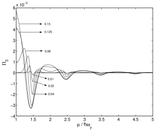
Figure 3: The third-order Peltier coefficient $\Pi_{3}$ (in arbitrary units) is plotted as a function of average chemical potential $\overline{\mu}$ for $\omega_{y}/\omega_{x}=6$ and different values of temperatures ($k_{B}\theta/\hbar\omega_{y}$ values are indicated in the figure).

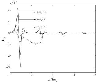
Figure 4: The third order Peltier coefficient $\Pi_{3}$ is plotted as a function of average chemical potential $\overline{\mu}$ for $k_{B}\theta/\hbar\omega_{y}=0.04$ and different values of $\omega_{y}/\omega_{x}$ whose values are indicated in the figure.

High-order nonlinearity in Peltier effect at small temperatures

As it was discussed above, highly nonlinear cases cannot be treated appropriately by the power series expansion discussed here. For this case, we need to have a better method for evaluating the heat and charge currents passing through the contact. We consider only the isothermal case appropriate for the Peltier effect. The charge and entropy currents for this case can be expressed as

$$I = 2\frac{(-e)}{h}\int_{-\infty}^{\infty}dx(-f^{\prime}(x))[A(\mu_{L}+xk_{B}\theta)-A(\mu_{R}+xk_{B}\theta)]\quad,$$ (28)

$$I_{S} = 2\frac{k_{B}}{h}\int_{-\infty}^{\infty}dx(-xf^{\prime}(x))[A(\mu_{L}+xk_{B}\theta)-A(\mu_{R}+xk_{B}\theta)]\quad,$$ (29)

where $A(E)$ is the energy integral of $T(E)$,

$$A(E)=\int_{-\infty}^{E}T(E)dE\quad.$$

Assuming small temperatures ($k_{B}\theta\ll E_{L}$), the integrands can be expanded as

$$A(\mu+xk_{B}\theta)\approx A(\mu)+xk_{B}\theta T(\mu)\quad.$$

Keeping only the lowest order terms the currents can be expressed as

$$I = 2\frac{(-e)}{h}(A(\mu_{L})-A(\mu_{R}))\quad,$$ (30)

$$\dot{Q} = \frac{2\pi^{2}}{3h}(k_{B}\theta)^{2}(T(\mu_{L})-T(\mu_{R}))\quad.$$ (31)

As was discussed by Bogachek et al.,bogachek1 ; bogachek2 the differential Peltier coefficient can be expressed as (assuming constant $\overline{\mu}$)

$$\Pi_{d}=\left(\frac{\partial\dot{Q}}{\partial I}\right)_{\overline{\mu}}=\frac{\pi^{2}(k_{B}\theta)^{2}}{3(-e)}\frac{T^{\prime}(\mu_{L})+T^{\prime}(\mu_{R})}{T(\mu_{L})+T(\mu_{R})}\quad.$$

The peak splitting effect of the nonlinearity can be seen from this expression. When the potential difference across the contact is less than $E_{L}$, the individual peaks of $T^{\prime}(\mu_{L})$ and $T^{\prime}(\mu_{R})$ will join in a single peak observed in the linear Peltier effect. However, if the potential difference is more than $E_{L}$, the contribution of these two terms can be distinguished since they will form two separate peaks. The distance between the peaks, then, will be proportional to the applied potential difference.

V Conclusions

The expansions of the charge and entropy currents as a power series in temperature and potential differences are obtained, assuming that the transmission probabilities are unchanged by the nonlinearities. The main advantage of this particular expansion is, through a different definition of average chemical potential, $\overline{\mu}$, and temperature, $\overline{\theta}$, some particular terms disappear from the expressions. The Seebeck and Peltier effects are investigated as special cases and it is found that the lowest order nonlinearities are of third order in both cases.

In the case of the Seebeck effect, $S_{3}$ is found to have the same sign as $S_{1}$. Although at low temperatures $S_{3}$ is found to be simply proportional to $S_{1}$, its peaks split into two at high temperatures. If $k_{B}\overline{\theta}$ is comparable to the energy difference between the successive sub-bands, these peaks may join with the peaks of the neighboring steps, creating an unusual appearance where $S_{3}$ has maxima at the plateaus of the conductance and minima at the steps. In all cases, it is found that the nonlinear signal is small compared to the linear one.

For the case of the Peltier effect, $\Pi_{3}$ changes sign as the gate voltage is changed for all parameter values. The main shortcoming of the expansion developed here is that in this case the potential difference driving the current may be chosen above the threshold level for nonlinearity. In such a case, the expansion is useless as more and more terms have to be added up to obtain the correct response. In the small temperature limit, an alternative expression has been developed for the differential Peltier coefficient that is also valid for highly nonlinear cases.

References

- (1) B. J. van Wees, H. van Houten, C. W. J. Beenakker, J. G. Williamson, L. P. Kouwenhoven, D. van der Marel, and C. T. Foxon, Phys. Rev. Lett. 60, 848 (1988).
- (2) D. A. Wharam, T. J. Thornton, R. Newbury, M. Pepper, H. Ahmed, J. E. F. Frost, D. G. Hasko, D. C. Peacock, D. A. Ritchie, and G. A. C. Jones, J. Phys. C: Solid State Phys. 21, L209 (1988).
- (3) R. Landauer, Philos Mag. 21, 863 (1970).
- (4) M. Büttiker, Y. Imry, R. Landauer and S. Pinhas, Phys. Rev. B 31, 6207 (1985).
- (5) P. Streda, J. Phys.: Condensed Matter 1, 1025 (1988).
- (6) C. R. Proetto, Phys. Rev. B 44, 9096 (1991).
- (7) H. van Houten, L. W. Molenkamp, C. W. J. Beenakker, C. T. Foxon, Semicond. Sci. Technol. 7, B215 (1992).
- (8) L. W. Molenkamp, H. van Houten, C. W. J. Beenakker, R. Eppenga, C. T. Foxon, Phys. Rev. Lett. 65, 1052 (1990).
- (9) L. W. Molenkamp, Th. Gravier, H. van Houten, O. J. A. Buijk, M. A. A. Mabesoone, C. T. Foxon, Phys. Rev. Lett. 68, 3765, (1992).
- (10) Z.-S. Ma, L. Schülke, Phys. Rev. B 59, 13209 (1998).
- (11) Z.-S. Ma, J. Wang, H. Guo, Phys. Rev. B 59, 7575 (1999).
- (12) Z.-S. Ma, H. Guo, L. Schülke, Z.-Q. Yuan, H.-Z. Li, Phys. Rev. B 61, 317 (2000).
- (13) B. Qiao, H. E. Ruda, Z. Xianghua, Physica A 311, 429 (2002).
- (14) T. N. Todorov, J. Phys.: Condensed Matter 12, 8995 (2000).
- (15) E. N. Bogachek, A. G. Scherbakov and U. Landman, Solid State Comm. 108, 851 (1998).
- (16) E. N. Bogachek, A. G. Scherbakov and U. Landman, Phys. Rev. B 60, 11678 (1999).
- (17) A.E. Krishnaswamy, S.M Goodnick, M.N. Wyborne, C. Berven, Microelectronic Engineering 63, 123 (2002).
- (18) A. S. Dzurak, C. G. Smith, L. Martin-Moreno, M. Pepper, D. A. Ritchie, G. A. C. Jones, and D. G. Hasko, J. Phys: Condens. Matter 5, 8055 (1993).
- (19) M. Büttiker, J. Phys: Condens Matter 5, 9361 (1993).
- (20) T. Christen and M. B ttiker, Europhys. Lett. 35, 523 (1996).
- (21) U. Sivan and Y. Imry, Phys. Rev. B 33, 551 (1986).