Dynamical transition for a particle in a squared Gaussian potential

Abstract

We study the problem of a Brownian particle diffusing in finite dimensions in a potential given by $\psi=\phi^{2}/2$ where $\phi$ is Gaussian random field. Exact results for the diffusion constant in the high temperature phase are given in one and two dimensions and it is shown to vanish in a power-law fashion at the dynamical transition temperature. Our results are confronted with numerical simulations where the Gaussian field is constructed, in a standard way, as a sum over random Fourier modes. We show that when the number of Fourier modes is finite the low temperature diffusion constant becomes non-zero and has an Arrhenius form. Thus we have a simple model with a fully understood finite size scaling theory for the dynamical transition. In addition we analyse the nature of the anomalous diffusion in the low temperature regime and show that the anomalous exponent agrees with that predicted by a trap model.

1 Introduction

Systems with quenched disorder are often taken as paradigms for systems exhibiting a structural glass transition. The basic physical idea is that for a sufficiently complex and frustrated system without quenched disorder, a single particle sees an effectively quenched and random potential due to the other particles. At a mean field level there exist models where, to all intents and purposes, this analogy becomes exact. One can have two models one with quenched disorder and the other without, but highly frustrated, which exhibit the same thermodynamics in the high temperature phase and the same glass transition at low temperatures [1]. Even if the frustrated non-random system possesses a crystalline ground state not shared by the disordered system, this fact is practically irrelevant as this state is dynamically never attained. An analogy between mean field spin glass models with one step replica symmetry breaking and structural glasses has been put forward [2, 3], and this theory of the glass transition has become known as the random first order scenario. Further extensions of the analogy between the dynamics of these mean field spin glasses and finite dimensional glass formers have provided much insight into glassy dynamics and related phenomena such as ageing and effective temperatures [3]. One of the simplest models, which has been extensively studied, is the so called toy model. Here one takes a particle in a $D$ dimensional space with Hamiltonian

$$H({\bf x})=\psi({\bf x})+{1\over 2}\mu{\bf x}^{2}\ ,$$ (1)

where $\psi$ is a quenched random potential taken from some statistical ensemble. The most convenient choice is to take $\psi$ to be Gaussian of zero mean with correlation function

$$\langle\psi({\bf x})\psi({\bf y})\rangle=\Delta(|{\bf x}-{\bf y}|),$$ (2)

so the field is statistically isotropic and invariant by translation in space. The statics of this model can be solved in the Gaussian variational approximation in finite dimensions [4]. This approximation becomes exact in limit of the number of spatial dimensions $D$ going to infinity if $\Delta$ scales as

$$\Delta(x)=DF({x^{2}\over D}).$$ (3)

In this limit when the correlation function of $F$ is short range a structural glass transition is found [4, 5]. First, at a temperature $T_{d}$ there is a dynamical transition, which is independent of the precise nature of the dynamics as long as it is local. This dynamical transition appears due to the appearance of an exponentially large number of metastable states and it can be located via static arguments, thus explaining its independence of the precise form of the local dynamics [5]. This transition is not accompanied by a strict thermodynamic transition. The thermodynamic transition appears at a lower temperature $T_{s}$ where the entropy of the system becomes very small. In the free case, where the harmonic confining potential is removed (the case $\mu=0$), a dynamical transiting occurs at a non-zero temperature, but the static transition is occurs only at $T=0$. The existence of the dynamical transition in the free case shows up as a transition between a stationary dynamics characterised by the time translational invariance of the correlation function and a form (for unbounded systems) of the fluctuation dissipation theorem [5] and a low temperature ageing regime exhibiting ageing in the correlation function and modified fluctuation dissipation relations [5]. In addition at high temperature the late time behaviour of a Brownian tracer particle in the force field generated by the potential is normal and is characterised by a non-zero diffusion constant which vanishes at $T_{d}$ [6]. A little thought convinces one that this is not possible in finite dimensions and that there is thus something pathological about the large $D$ limit as it is taken in this model. When the correlation length of the random field is finite (the case where the correlation function of the field is infinite is another matter and anomalous diffusion is clearly possible in this case) one can view the system on a coarse grained scale at the order of a few tens of this correlation length. We denote this length scale by $l_{*}$. The process can now be viewed as a discrete random walk between neighbouring regions with an exponentially distributed time to jump to a neighbouring region whose average is given by the Arrhenius law as $\tau=\tau_{0}\exp({\Delta E\over T})$. Here $\Delta E$ is the energy barrier associated with moving from one region to another. When the average value of $\tau$, $\overline{\tau}$ is finite the system will look like a random walk in the coarse grained picture and we find that

$$\langle{\bf X}_{t}^{2}\rangle\sim{l_{*}^{2}\over\overline{\tau}}\,t,$$ (4)

showing that we should have a finite diffusion constant. When $\psi$ is Gaussian we expect that the energy barriers $\Delta E$ are also Gaussian and thus obtain a value of $\overline{\tau}$ which behaves as

$$\overline{\tau}=\tau_{0}\exp\left({A\over T^{2}}\right),$$ (5)

which is referred to as a super-Arrhenius behaviour. The dynamical transition is however clearly relegated to zero temperature. This argument is backed up by numerical simulations, perturbative and renormalisation group calculations [6, 7]. In a finite system we will always have finite energy barriers and they will always be overcome by activated barrier hopping, all be it after very long but finite times. Mean field models have diverging energy barriers and it is this divergence which leads to the dynamical transition. Indeed the formula Eq. (5) should ultimately become Arrhenius-like for systems where the energy barrier are bounded and we will discuss this point in the next section on exact results.

A commonly used paradigm for glassy systems is the trap model [8] where the phase space is considered to be made up of a set of traps denoted by $i$ each of depth $\Delta E_{i}$. The simplest version is that where the traps are on a tree-like geometry, as is the case in the random energy model [8]. The generalised random energy model has traps within traps and is inspired by the Parisi solution for mean field spin glasses where the states (corresponding to the bottom of traps) are organised in with an ultra-metric structure [9]. The time spent in a trap is exponentially distributed with mean time $\tau_{i}=\tau_{0}\exp(\beta\Delta E_{i})$ and the distribution of the $\Delta E_{i}$ induces the distribution of the $\tau_{i}$. When the disorder averaged value of $\tau_{i}=\overline{\tau}$ diverges a dynamical transition occurs. Forms of the trap model where the traps are located on a finite dimensional lattice have been extensively studied [10, 11]. Also a non-random microscopic realisation, based on number partitioning combinatorics, of the trap model has been found [12]. Intuitively we expect the trap model picture to be applicable to the problem of a particle diffusing in a short range correlated random potential at sufficiently large time and length scales. In this paper we show that for the model we study this is indeed the case.

Going back to the problem of diffusion in a random potential, we consider a model where $\psi=\phi^{2}/2$ where $\phi$ is Gaussian. Clearly from the arguments above we do expect to see a dynamical/glass transition. We assume that the potential energy barriers also behave as the energy itself, we thus assume that the statistics of the barrier heights behaves as $\alpha\phi^{2}/2$, where $\alpha$ is some positive constant. Therefore average time spent in a trap will behave as

$$\tau\sim\tau_{0}\exp({\beta\alpha\phi^{2}\over 2})$$ (6)

If we take a Gaussian field $\phi$ with correlation function

$$\langle\phi({\bf x})\phi({\bf y})\rangle=\Delta({\bf x}-{\bf y})$$ (7)

with $\Delta(0)=1$, then $\overline{\tau}$ diverges for $\beta\alpha>1$, giving a dynamical transition temperature $T_{g}=\alpha$. Note that in [13] the problem of a dipole diffusing in a Gaussian electrostatic field $\psi$ was considered. Here the effective potential felt by the dipole is $\psi=-{1\over 2}(\nabla\phi)^{2}$. The above argument indicates that a dynamical transition, indicated by a vanishing of the diffusion constant, should occur in this model. However in [13] no clear evidence for a phase transition was found in numerical simulations in three dimensions. However standard methods for generating the Gaussian field used here and in [13] use a finite number of Fourier modes. Indeed we will show that, in the case studied here where exact results are possible, there is a finite size scaling in the number of modes $N$. This finite size scaling smears out the dynamical transition, just as is the case in the standard theory of equilibrium second order phase transitions.

The Langevin of dynamics we shall study of a particle in a potential $\psi$ is given by,

$$\dot{\bf X}_{t}={\bf\eta}(t)-\beta\nabla\psi({\bf X}_{t})$$ (8)

where $\eta(t)$ is Gaussian white noise with correlation function

$$\langle\eta_{i}(t)\eta_{j}(t^{\prime})\rangle=2\delta_{ij}\delta(t-t^{\prime}).$$ (9)

This choice of white noise amplitude ensures that the stationary measure is the Gibbs-Boltzmann equilibrium one. The diffusion constant, when it exists, of the system is defined by the late time behaviour of the mean squared displacement as

$$\langle{\bf X}^{2}_{t}\rangle\sim 2D\kappa_{e}t.$$ (10)

Therefore using this notation the bare diffusion constant of the particle in the absence of the field $\psi$ will always be given by $\kappa_{e}=\kappa_{0}=1$.

We will find here that the low temperature phase is characterised by an anomalous sub-diffusive behaviour

$$\langle{\bf X}^{2}_{t}\rangle\sim t^{2\nu},$$ (11)

where the exponent associated with the anomalous diffusion $\nu<1/2$. We then argue that the problem can be mapped onto an effective trap model which allows us to predict the value of $\nu$. This prediction, in one dimension, is confirmed by a formal replica calculation applied to a first passage time problem. It is also supported by our numerical results.

2 Exact Results

The diffusion constant for a particle in a one dimensional random potential, which is statistically invariant under translation, can be obtained exactly in a number of ways [14, 15]. It is given by

$$\kappa_{e}={1\over\langle\exp\left(\beta\psi\right)\rangle_{d}\langle\exp\left(-\beta\psi\right)\rangle_{d}},$$ (12)

where the subscript $d$ indicates the disorder average over the field $\psi$ taken at any point. An interesting point about this formula is that the resulting $\kappa_{e}$ is independent of the sign of $\beta$. In the case where $\psi=\phi^{2}/2$ where the one-point distribution function for $\phi$ is Gaussian and given by

$$p(\phi)={1\over\sqrt{2\pi}}\exp(-\phi^{2}/2)$$ (13)

we have the result

$$\kappa_{e}=\sqrt{1-\beta^{2}}$$ (14)

and so at $\beta_{g}=1$ a dynamical transition thus occurs where the diffusion constant becomes zero. This transition is really present, and below this transition temperature the diffusion will become anomalous.

Note that if the energy barrier corresponding to a coarse grained region is given by $\alpha\phi^{2}\over 2$ with the distribution of $\phi$ given by equation (13), then the induced distribution on the trapping time $\tau$ given by equation (6) is

$$\rho(\tau)={\tau_{0}^{1\over\alpha\beta}\over\tau^{1+{1\over\alpha\beta}}\sqrt{\pi\alpha\beta\ln({\tau\over\tau_{0}})}}.$$ (15)

The above trapping time distribution is almost Levy like apart from the logarithmic term. Below the critical temperature given by $\alpha\beta_{c}=1$ we see that the mean value diverges, as can be seen directly. The trap model has been extensively studied in finite dimensions in this regime. The precise definition is as follows, the system consists of a series of traps on a finite dimensional lattice. Associated with each site $i$ is an trap whose residence time, the time before the next jump is made, is exponential with quenched mean $\tau_{i}$. If the distribution of the $\tau_{i}$ are independent and identically distributed with distribution

$$\rho(\tau)\approx A{\tau_{0}^{\mu}\over\tau^{\mu+1}}$$ (16)

then we see that $\overline{\tau_{i}}$ diverges for $\mu<1$. For $\mu>1$ in one dimension we have that

$$\langle{\bf X}_{t}^{2}\rangle\sim C\ t\ \;;\mu>1$$ (17)

which is normal diffusion. In the anormal phase, $\mu<1$ the mean squared displacement behaves as [16]

$$\langle{\bf X}_{t}^{2}\rangle \sim C\ t^{2\mu\over\mu+1}\ \;;D=1$$ (18)

$$\sim C\ t^{\mu}(\ln(t))^{1-\mu}\ \;;D=2$$

$$\sim C\ t^{\mu}\ \;;D>2.$$

From equation (15) we see that up, to logarithmic corrections, the model studied here should correspond to a trap model where the exponent of this anomalous diffusion is given by

$$\mu=\frac{1}{\alpha\beta}.$$ (19)

The low temperature phase of the model should thus be characterised by anomalous diffusion. In fact, in what follows, we shall see, both from analytic arguments and numerics, that the effective value of $\alpha$ in all the above is in fact $1$. The difficulty of trap models with quenched disorder is that a particle may in general visit a trap several times and thus it is not necessarily a good approximation to draw a new $\tau_{i}$ from the quenched distribution each time an already visited site is revisited. This approximation is called the annealed approximation and fails badly in one and two dimensions where the random walk is recurrent [16]. The model corresponding to the annealed approximation is the annealed model where each time a particle visits a site the trapping time is redrawn from the distribution of waiting times (which is site independent). Above the critical value $\mu_{c}=1$ the annealed model in one dimension diffuses as

$$\langle{\bf X}_{t}^{2}\rangle\sim C\ t+O(\sqrt{t})\ \;;\mu>2.$$ (20)

However, still above $\mu_{c}=1$ but with $1<\mu<2$ we find

$$\langle{\bf X}_{t}^{2}\rangle\sim C\ t+O(t^{1\over\mu})\;;1<\mu<2.$$ (21)

This change in the exponent of the sub-leading temporal behaviour stems from the fact that the variance of the time spent in a trap ${\overline{\tau}_{i}^{2}}-{\overline{\tau}_{i}}^{2}$ diverges, while the mean value remains finite. Thus we see that there are two regimes of normal diffusion, a high temperature one corresponding to $\mu>2$ as given by equation (20) and a low temperature normal phase with $1<\mu<2$ and where the corrections to pure diffusion change from $O(\sqrt{t})$ to $O(t^{\frac{1}{\mu}})$. The key point is the divergence of the variance of the trapping time at a given site and we thus expect a similar transition to occur in the quenched version of the model. For $\mu<1$ the annealed model gives

$$\langle{\bf X}_{t}^{2}\rangle\sim Ct^{\mu}$$ (22)

in all dimensions. Thus we see that, in low dimensions, the exponent associated with the anomalous diffusion in the annealed model is not the same as that associated with the quenched model. This is precisely due to the recurrence of random walks in two and less dimensions.

For our later comparison with numerical simulations we will need to compute the correction to normal diffusion in the high temperature limit. As random walks are recurrent in one dimension transient effects are very important and unless one can predict them the extraction of a diffusion constant from a numerical simulation becomes extremely difficult.

In the high temperature phase we write

$$\langle{\bf X}_{t}^{2}\rangle\sim 2\kappa_{e}t+O(t^{\theta}).$$ (23)

Now if the corresponding trap model is characterised by $\alpha=1$ then we have $\mu=1/\beta$. Adapting the scaling argument found in [16] to the finite time corrections we predict that

$$\theta = 3/4\ {\rm for}\ \mu>2$$ (24)

$$= {1\over 2}+{1\over 2\mu}={\beta+1\over 2}\ {\rm for}\ 1\leq\mu\leq 2,$$

The above results for the exponent $\theta$ turn out to be in good agreement with our numerical results. This supports both our scaling arguments and the identification of our model with a trap model characterised by the exponent $\mu=1/\beta$ (equivalently $\alpha=1$). The prediction of equation (24) shows that the finite time corrections to diffusion are always important, and as one approaches the transition at $\beta=1$ they become of the same order as the normal diffusion term.

Returning to the Langevin problem one may be tempted to argue that the transition seen in one dimension could be rather pathological in that the system is obliged to overcome all energy barriers in one dimension. Unfortunately no general exact results exist in higher dimensions, however in two dimensions if the field $\psi$ is statistically the same as $-\psi$ a duality argument can be used [17] (in a rather indirect way) to show that

$$\kappa_{e}={1\over\langle\exp\left(-\beta\psi\right)\rangle_{d}}.$$ (25)

This clearly allows us to compute $\kappa_{e}$ in two dimensions in the case where $\psi$ Gaussian. We can however get an exact result for another potential by judiciously choosing a field of the form

$$\psi={\phi^{2}\over 2}-{\phi^{\prime 2}\over 2},$$ (26)

where $\phi$ and $\phi^{\prime}$ are independent Gaussian fields with the same statistics. Clearly $\psi\sim-\psi$ in the statistical sense and we thus obtain the exact result

$$\kappa_{e}=\sqrt{1-\beta^{2}},$$ (27)

showing that the same dynamical transition occurs in two dimensions for this particular choice of $\psi$.

If one wants to simulate the Langevin process considered here on a computer, without resorting to a lattice model, one may use a standard method to generate a Gaussian random field [18], where one takes

$$\phi=\sqrt{{2\over N}}\sum_{n=1}^{N}\cos({\bf k}_{n}\cdot{\bf x}+\epsilon),$$ (28)

where $N$ is the number of modes chosen. When, as we assume here, $\Delta(0)=1$ one takes each wave vector ${\bf k}_{n}$ independently from the distribution

$$P({\bf k})={1\over(2\pi)^{D}}\int d{\bf x}\,\exp(i{\bf k}\cdot{\bf x})\Delta({\bf x}).$$ (29)

For instance here we will carry out simulations with

$$\Delta({\bf x})=\exp(-{{\bf x}^{2}\over 2})$$ (30)

and so each component of a vector ${\bf k}_{n}$ is a Gaussian of mean zero and variance one. In the limit of large $N$ the field so generated becomes Gaussian but it is interesting to see what the effect of a finite number of modes is from both a theoretical and practical (for comparison with numerical simulations) point of view. We start with the simple Gaussian case where we have

$$\langle\exp\left(\beta\phi\right)\rangle_{d}=\left[{1\over 2\pi}\int_{0}^{2\pi}d\epsilon\,\exp\left(\beta\sqrt{2\over N}\cos(\epsilon)\right)\right]^{N}=I_{0}\left(\beta\sqrt{2\over N}\right)^{N}\ ,$$ (31)

where $I_{0}$ is a modified Bessel function [19]. The function $I_{0}$ has the small $z$ behaviour given by [19]

$$I_{0}(z)=1+{{1\over 4}z^{2}\over(1!)^{2}}+{({1\over 4}z^{2})^{2}\over(2!)^{2}}+O(z^{6})\ ,$$ (32)

and the large $z$ asymptotic behaviour [19]

$$I_{0}(z)={\exp(z)\over\sqrt{2\pi z}}\left[1+O({1\over z})\right].$$ (33)

From equation (32) we thus find that in the limit $N\to\infty$ but keeping $\beta$ finite we find

$$\kappa_{e}=\exp(-{\beta^{2}})=\exp(-{1\over T^{2}})$$ (34)

in one dimension. We thus obtain the super-Arrhenius law associated with as expected. However at much lower temperatures such that $\beta\gg N^{2}$ we use the asymptotic form equation (33) to obtain

$$\kappa_{e}=\left({8\pi^{2}\beta^{2}\over N}\right)^{1\over 2}\exp\left(-2\beta\sqrt{2N}\right)\sim\exp(-{2\sqrt{2N}\over T})$$ (35)

and thus we recover the Arrhenius law at extremely low temperatures. Note that the term $\Delta E$ in equation (35) is simply the maximal difference in energy possible for the field $\phi$ expressed as a finite Fourier series as in equation (28).

As stated earlier when $\psi=\phi$ we have the statistical equivalence necessary to use the result equation (25) and we find the corresponding two dimensional results

$$\kappa_{e}=\exp(-{\beta^{2}\over 2})=\exp(-{1\over 2T^{2}})$$ (36)

for $N\to\infty$ and $\beta$ finite , and

$$\kappa_{e}=\left({8\pi^{2}\beta^{2}\over N}\right)^{1\over 4}\exp\left(-\beta\sqrt{2N}\right)\sim\exp(-{\sqrt{2N}\over T}),$$ (37)

for $\beta\gg N^{2}$. We see again that the Arrhenius law is recovered in this limit, but in contrast with the one dimensional case, the term $\Delta E$ in equation (37) is only half of the maximal energy difference between two points. This makes sense as in two dimensions one can go around this maximal energy barrier.

The case of a squared Gaussian potential is treated similarly using

$$\langle\exp(\beta\psi)\rangle_{d} = \int_{-\infty}^{\infty}{dz\over\sqrt{2\pi}}\exp(-{z^{2}\over 2})\langle\exp(z\sqrt{\beta}\phi)\rangle_{d}$$ (38)

$$= \int_{-\infty}^{\infty}{dz\over\sqrt{2\pi}}\exp(-{z^{2}\over 2})I_{0}\left(z\sqrt{2\beta\over N}\right)^{N}$$

$$= \sqrt{{N\over 2\pi}}\int_{-\infty}^{\infty}du\exp\left(Nf(u)\right)$$

where

$$f(u)=-{u^{2}\over 2}+\ln\left[I_{0}\left(u\sqrt{2\beta}\right)\right].$$ (39)

The integral in equation (38) can now be treated in the saddle point approximation. From the small $z$ expansion of $I_{0}$ of equation (32) we see that, about $u=0$, $f(u)$ takes the form

$$f(u)=-(1-\beta){u^{2}\over 2}-\beta^{2}{u^{4}\over 16}+O(u^{6}).$$ (40)

We therefore see that the dynamical transition occurring at $\beta=1$ is mathematically equivalent to a mean field ferromagnetic transition ! Note that if $\beta$ is negative then no transition occurs so the term $\langle\exp(-\beta\psi)\rangle$ behaves analytically as $N\to\infty$. In the high temperature phase $\beta<1$ therefore we have

$$\langle\exp(\beta\psi)\rangle_{d}={1\over\sqrt{1-\beta}}\left[1-{3\over N(1-\beta)^{2}}+O({1\over N^{2}})\right]\ ,$$ (41)

which gives

$$\kappa_{e}=\sqrt{1-\beta^{2}}\left[1+{3\beta^{2}\over 8N}{\beta^{2}+1\over(1-\beta^{2})^{2}}+O({1\over N^{2}})\right].$$ (42)

When $\beta>1$ the saddle point is no longer at $u=0$ and the function $f$ has a maximum value greater than zero at the points $\pm u_{c}$ where the maximum is attained. Here we find that

$$\kappa_{e}={1\over 2}\sqrt{(1+\beta)|f^{\prime\prime}(u_{c})|}\exp\left(-Nf(u_{c})\right).$$ (43)

For $\beta\sim 1$ we find that $u_{c}=2\sqrt{\beta-1}/\beta$ and consequently

$$\kappa_{e}={1\over 2}\sqrt{2(\beta^{2}-1)}\exp\left(-N{(\beta-1)^{2}\over\beta^{2}}\right).$$ (44)

At low temperatures we can use the asymptotic behaviour in equation (33) to obtain $u_{c}\approx\sqrt{2\beta}$ and thus

$$\kappa_{e}={1\over 2}\sqrt{(1+\beta)}\exp\left(-\beta N\right)\sim\exp\left(-{N\over T}\right).$$ (45)

Again note that that the last part of the above equation indicates an Arrhenius law corresponding to the maximum difference in energy between two points, the lowest value of $\psi$ being zero and the maximum being $N$. In two dimensions for the symmetric potential of equation (26) we find exactly the same results as for the one dimensional potential.

To give the reader a feel for what happens when the number of modes is finite we have plotted the $N=\infty$ result, equation (14), against the corresponding results for $N=64$ and $N=128$, often considered to be sufficient for simulation purposes, which are evaluated numerically using the exact equation (38). We see that even for $N=128$ that the value of $\kappa_{e}(1)$ is still of order 1 !

Given the above, it is interesting to examine the case of a diffusing dipole as studied in [13]. In the case of positive temperature the potential $\psi=-{1\over 2}(\nabla\phi)^{2}$ has localised minima of varying depths which can be regarded as traps. Therefore in this case one would think that the trap model picture would be a reasonably good approximation. If we take the equation (6) with $\alpha=1$ and apply it to this case (authors of [13] used $\Delta({\bf x})=\exp(-{\bf x^{2}}/2)$) one finds that the transition occurs at $\beta=1$. Interestingly the numerical results of [13] indicate a cross over from a concave behaviour to a convex behaviour of $\kappa_{e}$ in this region, rather reminiscent of the behaviour of the finite $N$ values in figure (1) near the dynamical transition. It is also interesting to note that the third and fourth order perturbation theory results of [13] give values of $\kappa_{e}$ which vanish close to $\beta=1$ (extremely close in the case of the third order result). Having said this we have no rigorous proof that there should be a transition in the model studied in [13]. However, for the reasons presented here, a finite size scaling analysis could resolve this issue. In [13] there is no evidence for a transition at negative temperatures.

Figure 1: Exact value of the diffusion constant $\kappa_{e}$ in one dimension for a squared potential. The solid line shows the exact Gaussian result ($N=\infty$ modes) and the dotted and dashed lines are for $N=128$ and $N=64$ modes respectively. Note that at the Gaussian transition temperature given by $\beta=1$ the corresponding $\kappa_{e}$ for $N=128$ modes is $\kappa_{e}(1)\approx 0.3$

To summarise, our exact results have shown that, in the squared Gaussian cases studied here, the high temperature regime is characterised by a relaxation time $\tau$ (using the fact that the correlation length scale is O(1)) which is finite but diverges as $T\to T_{g}$ as

$$\tau\sim{1\over(T-T_{g})^{{1\over 2}}}.$$ (46)

However when the potential is constructed from a finite number of modes we find that for $T<T_{g}$.

$$\tau\sim\exp({N\Delta\epsilon(T)\over T})$$ (47)

where $N\Delta\epsilon(T)$ can be interpreted as a temperature dependent energy barrier. In one dimension this barrier height tends to the maximal difference in potential possible between two points as the temperature approaches zero and in two dimensions it tends to half the maximal difference.

In one dimension one can obtain information about transport behaviour by analysing first passage time. This method can be used to calculate the diffusion constant in a one dimensional potential [14] and was used in [20] to determine the exponents of the anomalous diffusion in a Gaussian potential with long range (logarithmic) correlations. To simplify the calculation one considers diffusion on the half line with reflecting boundary conditions at the origin $0$. We denote by $T(L)$ the average (in the thermal sense of averaging over realisations of the white noise) time at which the tracer particle starting at the origin first reaches the point $L$. This average first passage time is given by (see [20] and references within) the following double integral which depends on the realisation of the driving field $\psi$

$$T(L)=\int_{0}^{L}dydx\;\theta(y-x)\exp\left(\beta\psi(y)-\beta\psi(x)\right).$$ (48)

In general we can compute the moments of $T$ by replicating the double integrals to yield upon disorder averaging

$$\overline{T(L)^{n}}=\int_{0}^{L}\prod_{a}dy_{a}dx_{a}\theta(y_{a}-x_{a})\det\left(I+\beta A\Lambda\right)^{-{1\over 2}},$$ (49)

where the matrices $A$ and $\Lambda$ are symmetric $2n\times 2n$ matrices with

$$A_{ab}=\Delta(y_{a}-y_{b})$$ (50)

and

$$\Lambda_{ab} = -\delta_{ab}\ \ \ {\rm for}\ 1\leq a,b\leq n$$ (51)

$$= 0\ \ \ {\rm for}\ 1\leq a\leq n,\ n+1\leq b\leq 2n$$

$$= \delta_{ab}\ \ \ {\rm for}\ n+1\leq a,b\leq 2n,$$

where we have used the notation $x_{a}=y_{n+a}$. For the first moment $n=1$ we find, where it is finite, that

$$\overline{T(L)}=\int_{0}^{L}\prod dydx\;\theta(y-x){1\over\left(1-\beta^{2}+\beta^{2}\Delta^{2}(y-x)\right)^{1\over 2}}$$ (52)

For $\beta<1$ we may write

$$\overline{T(L)}={1\over 2L^{2}\sqrt{1-\beta^{2}}}+\int_{0}^{L}dydx\;\theta(y-x)\left({1\over\left(1+{\beta^{2}\over 1-\beta^{2}}\Delta^{2}(y-x)\right)^{1\over 2}}-1\right),$$ (53)

which becomes for large $L$,

$$\overline{T(L)}={L^{2}\over 2\sqrt{1-\beta^{2}}}-LC$$ (54)

where

$$C=\int_{0}^{\infty}dz\;\left[1-{1\over\left(1+{\beta^{2}\over 1-\beta^{2}}\Delta^{2}(z)\right)^{1\over 2}}\right]$$ (55)

when it is finite. The leading order in $L$ of the right hand side above yields the correct high temperature diffusion constant.

Inspection of the double integral in equation (52) shows that, assuming that $\Delta(x)$ is monotonically decreasing, the value of ${\overline{T}(L)}$ is finite as long as $\Delta(L)^{2}>(\beta^{2}-1)/\beta^{2}$. This is clearly always the case in the high temperature phase $\beta<1$. In the low temperature phase there is now a length scale $L_{c}$, which is temperature dependent: for $L<L_{c}$ $\overline{T(L)}$ is finite, and for $L>L_{c}$ it is divergent. For a monotone $\Delta$ this means that $L_{c}$ decreases with temperature and we may tentatively relate this with the idea of the system progressively freezing on smaller and smaller length scales as the temperature is decreased. This image of the system becoming frozen on smaller and smaller length scales is one which has been used extensively to interpret experiments on spin glasses [21].

We will now present an argument which will give a prediction for the exponent of anomalous diffusion in the low temperature phase. The argument is similar in spirit to that of [20] for long range Gaussian potentials in one dimension, although it is difficult to make it as rigorous as in the long range case. First notice that as one approaches the transition temperature the terms causing the divergence in equation (52) are those where $x$ and $y$ are far away from each other and hence uncorrelated. Secondly note that in the equation (48) we expect (in the case of $\beta>0$) that the first passage time is dominated by the maximal value of $\phi$. Let us denote this value by $y_{*}$. In the replicated averaged formula equation (49) we thus expect the most divergent term to occur at $y_{a}=y_{*}$ for all $a$. Also we expect that their are many values of $x$ which contribute to the most divergent term in equation (49) and these are points where $\phi(x)=0$. In general theses points will be well separated and far from $y_{*}$. Thus over most of the replicated interval $|x_{a}-x_{b}|\gg 1$ and $|x_{a}-y_{*}|\gg 1$. This means that one can make the approximation in the integral that $\Delta(x_{a}-x_{b})\approx 0$ and $\Delta(x_{a}-y_{*})\approx 0$ and thus the replicated integral in equation (49) can be approximated as

$$\overline{T(L)^{n}} \approx \int_{0}^{L}dy_{*}\int_{0}^{y_{*}}dx_{a}\det\left(I+\beta B\Lambda\right)^{-{1\over 2}}$$

$$\approx \det\left(I+\beta B\Lambda\right)^{-{1\over 2}}\ {L^{n+1}\over n+1}$$

where

$$B_{ab} = -1\ \ \ {\rm for}\ 1\leq a,b\leq n$$ (57)

$$= 0\ \ \ {\rm for}\ 1\leq a\leq n,\ n+1\leq b\leq 2n$$

$$= \delta_{ab}\ \ \ {\rm for}\ n+1\leq a,b\leq 2n,$$

The eigenvalues of $B$ are easily calculated, there being $1$ equal to $-n\beta$, $n-1$ equal to $0$ and $n$ equal to $1$.

This now gives

$$\overline{T(L)^{n}}\approx{1\over(1+n)(1-n\beta)^{1\over 2}(1+\beta)^{n\over 2}}L^{n+1}$$ (58)

Now if we choose the exponent $n$ to be very close to ${1\over\beta}$ we find that the equation (58) is indeed diverging and should be the dominant contribution. This yields

$$\overline{T(L)^{1\over\beta}}\sim L^{1+{1\over\beta}}$$ (59)

and thus dimensionally we have

$$\langle X_{t}^{2}\rangle\sim t^{2\over 1+\beta}$$ (60)

in agreement with the arguments in [11] and references therein.

In the presence of an external field the potential becomes ${1\over 2}\psi^{2}-hx$. The same line of reasoning now gives for large $L$

$$\overline{T(L)^{n}} \approx \int_{0}^{L}dy_{*}\int_{0}^{y_{*}}dx_{a}\exp\left(-nhy_{*}+\sum_{a}hx_{a}\right)\det\left(I+\beta B\Lambda\right)^{-{1\over 2}}$$

$$\approx \det\left(I+\beta B\Lambda\right)^{-{1\over 2}}{L\over(\beta h)^{n}}.$$

Again we set $n$ very close to ${1\over\beta}$ and dimensionally find the form

$$\langle X_{t}\rangle\sim h^{1\over\beta}t^{1\over\beta}$$ (62)

again in agreement with the results of [11], not only for the temporal exponent but also for the exponent associated with $h$. The above calculation also show that the value of $\alpha$ associated with the effective trap model defined by equation (6) for this problem is indeed $\alpha=1$.

3 Numerical Simulations

In this section we will verify the analytical results of the previous sections via two distinct types of numerical simulations. We begin with a direct simulation of the Langevin process using a second order Runga-Kutta integration of the Langevin equation as developed in references [22] and generating the random field $\phi$ via equation (28) as proposed originally in [18]. This simulation technique allows access to the asymptotic regime, where the relevant transport coefficients can be evaluated, at high temperatures in the regime of normal diffusion and at temperatures below $T_{g}$, but not too low. Clearly in order to attain the asymptotic regime at low temperatures we need to diffuse over a sufficiently large distance. However as the diffusion becomes progressively slower the times needed to attain this regime become prohibitive from the computational point of view. We expect that the low temperature phase should be described by a one dimensional trap model but, as discussed above, it is not completely obvious what parameters we should take for this trap model. We have therefore constructed an effective trap model directly from a realisation of the random field as generated by equation (28). The procedure used is the following. We take a realisation of the field $\psi$ over a suitably large interval. Each minima $\alpha$ of the field is associated with a point $\alpha$ on the line at its actual position denoted by $x_{\alpha}$. We then calculate the energy barrier to move to the nearest minima to the left $\alpha-1$ and the right $\alpha+1$. These two energy barriers are denoted by $\Delta E_{\alpha}^{(L)}$ and $\Delta E_{\alpha}^{(R)}$ respectively. The particle then is taken to jump to the left/right at an exponentially distributed random time $T_{L/R}$ with average value given by the Arrhenius law $\tau_{L/R}=\exp\left(\beta\Delta E_{\alpha}^{(L/R)}\right)$ (the over all scaling of time is unimportant to determine the exponent associated with the anomalous diffusion). From the site $\alpha$ $T_{L/R}$ are generated numerically and the particle hops to the site corresponding to the shorter time. The time of the simulation is then increased by this shorter time. In this way we can assure that the system has diffused sufficiently far and the total simulation time is independent of the physical time, allowing us to attain the asymptotic regime.

Our numerical integration of the stochastic differential in the high temperature normal phase yields the following results. Shown in figure (2) is the value of the diffusion constant $\kappa_{e}$ determined from a fit $\langle X^{2}_{t}\rangle=2\kappa_{e}t+Bt^{\theta}$, where $\theta$ is the exponent predicted by equation (24). The numerical result is generated by averaging over $10000$ particles in each realisation of the random field and averaging over $100$ realisations generated using $128$ modes. The total time of the simulation consisted of $5000$ integration steps using $\Delta t=0.5$ in the second order stochastic Runga-Kutta. Again we see that the above fit is in good agreement with the theoretical result for $N=128$ (dashed line) modes. Also shown is the $N\to\infty$ result (solid line)

Figure 2: Fit of simulation results (circles), assuming an exponent $\theta$ given by equation (24), of the diffusion constant $\kappa_{e}$ in one dimension using $N=128$ modes. The dashed line shows the analytic result for $N=128$ modes and the solid line that in the limit $N\to\infty$.

In figure (3) we show the fitted value of the exponent $\theta$ assuming the exact result (for $N=128$ modes) for $\kappa_{e}$. We see that the result is in good accord with the scaling prediction of equation (24) for $\theta$.

Figure 3: Fit of simulation results (circles), of the exponent $\theta$, using the analytic result for $\kappa_{e}$ in one dimension with $N=128$ modes. The solid line shows the scaling prediction equation (24) for $\theta$.

For temperatures not too far below $T_{g}$ we may use a direct numerical integration to estimate the exponent $\nu$. The results of these simulations are shown in figure (4) (empty squares). We see that the numerically measured value of the exponent is close to the predicted one up to $\beta\sim 1.5$ but after it departs from the predicted value. We believe that this because we are not carrying out the simulation for sufficiently long times. Indeed when we simulate the trap model, where simulation time is no longer a problem, we see from figure (4) (filled circles) that the agreement with the theoretical result is much improved for the larger values of $\beta$.

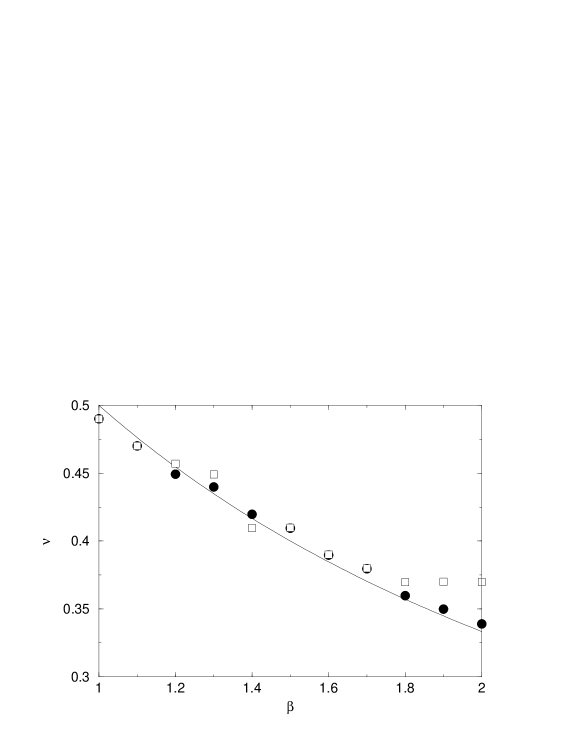
Figure 4: Fit of exponent of anomalous diffusion $\nu$ obtained from the one dimensional effective trap model (circles) and direct integration of the stochastic differential equation (squares) shown against the prediction $\nu=1/(1+\beta)$ (solid line).

4 Conclusions

We have studied the dynamics of a particle diffusing in an potential which is given by the square of a Gaussian potential whose statistics are translationally invariant in space and whose correlation function is short ranged. In contrast to the Gaussian case, there really is a dynamical transition for this model. The transition manifests itself as a crossover between a high temperature diffusive regime and a low temperature regime where the particle diffusion is anomalous and more specifically is sub-diffusive. We showed how the diffusion constant could be computed in one dimension and in a special case in two dimensions. Interestingly when the Gaussian field is constructed using a finite Fourier series we see that, instead of vanishing at the dynamical transition temperature, the diffusion constant obeys an Arrhenius form dependent on the maximal energy barrier present in the system, Explicitly we have shown

$$\kappa_{e}\sim C\exp(-{AN\over T}),$$ (63)

at low temperatures. This result is physically intuitive and our calculation allows for a complete understanding of the finite size scaling underlying this dynamical transition. We also showed that these finite scaling effects can be important for the number of modes typically used in numerical simulations. In addition, in one dimension we show that the low temperature phase can be described in terms of a trap model where the energy barriers are assumed to have the same statistics as the energy function itself. The resulting sub-diffusive behaviour for the low temperature regime in one dimension is

$$\langle X^{2}_{t}\rangle\sim t^{2\over 1+\beta}.$$ (64)

This scaling, form and that for the mean displacement in the presence of a uniform drift was also obtained via a, non-rigorous, replica based computation of the moments of the mean first passage time. Finally in the case of a finite number of modes it is a natural question ask which time scale must one go to in order to see the finite size effect diffusive behaviour in the low temperature regime as opposed to anomalous diffusion. A simple way to estimate this cross over time $t_{c}$ is to equate the mean squared displacements in the anomalous and diffusive cases, i.e.

$$t_{c}^{2\over 1+\beta}\sim\exp(-{AN\over T})\ t_{c},$$ (65)

which yields at low temperatures

$$t_{c}\sim\exp\left({AN\over T}\right).$$ (66)

Acknowledgments: DSD would like to thank the Isaac Newton Institute Cambridge where part of this work was carried out during the programme Principles of the Dynamics of Non-Equilibrium Systems. We would also like to thank J.-P. Bouchaud for useful conversations and pointing out the interest of this model.

References

References

- [1] Marinari E, Parisi G and Ritort F 1994 . J. Phys. A 27 7615; Marinari E, Parisi G and Ritort F 1994 J. Phys. A 27 7647; Bouchaud J-P and Mezard M (1994) J. Phys. I 4 1109
- [2] Kirkpatrick T R and Thirumalai D 1987 Phys. Rev. B 36 5388
- [3] Bouchaud J-P , Cugliandolo L F, Kurchan J and Mézard M 1998 Out of Equilibrium dynamics in spin-glasses and other glassy systems, in Spin-glasses and Random Fields edited by A. P. Young (World Scientific)
- [4] Mézard M and Paris G 1991 J. Phys. I France 1 809; Engel A 1993 Nucl. Phys. B, 410 617; Fyodorov Y V and Sommers H-J cond-mat/0610035
- [5] Franz S and Mézard M 1994 Physica A 210 48; Cugliandolo L F and Le Doussal P 1996, Phys. Rev. E 53 1525; Kinzelbach H and Horner H 1993 J. Phys. I 3 1329
- [6] Dean D S, Drummond I T, Horgan R R and Da-Silvo-Santos C A 1998, Europhys. Lett. 42 241
- [7] Dean D S, Drummond I T and Horgan R R 1994 J. Phys. A: Math Gen 27 5135; Deem M W and Chandler D 1994 J. Stat. Phys. 76 911
- [8] Bouchaud J-P 1992 J. Phys. I 2 1705
- [9] Bouchaud J-P and Dean D S 1995 J. Phys. I 5, 265
- [10] Monthus C 2004 Phys. Rev. E, 69 026103; Monthus C 2003 Phys. Rev. E, 67 046109; Monthus C 2003 Phys. Rev. E, 68 036114; Ben Arous G and Cerny J 2005 Ann. App. Prob, 15 1161, Monthus C and Bouchaud J-P 1996 J. Phys. A 29 3847; Monthus C 2003 J. Phys. A 36 11605
- [11] Bertin E and Bouchaud J-P 2003 Phys. Rev. E 67 065105; Bertin E and Bouchaud J-P 2003 Phys. Rev. E 67 026128
- [12] Junier I and Kurchan J 2004 J. Phys. A, 37 3945
- [13] Drummond I T, Horgan R R and da Silva Santos C A 1998 J. Phys. A: Math Gen 30 1341
- [14] Zwanzig R 1988 Proc. Natl. Acad. Sci USA 85 2029
- [15] Dean D S, Drummond I T , Horgan R R and Lefèvre A 2004 J. Phys. A. 37 10459
- [16] Bouchaud J-P and Georges A 1990 Phys. Reps 195 127
- [17] Dean D S, Drummond I T and Horgan R R 1997 J. Phys. A: Math Gen 30 385; Dean D S, Drummond I T and Horgan R R 2004, J. Phys. A. 37 2039
- [18] Kraichnan R H 1976 J. Fluid. Mech. 77 753
- [19] Abramowitz M and Stegun I A (Eds) 1964 Handbook of Mathematical Functions Dover (New York)
- [20] Castillo H E and Le Doussal P 2001 Phys. Rev. Lett 86 4859
- [21] Bouchaud J-P, Dupuis V, Hammann J and Vincent E 2002 Phys. Rev. B 65 024439; Berthier L and Holdsworth P C W 2002 Europhys. Lett. 58 35; Bethier L and Bouchaud J-P 2002 Phys. Rev. B 66 054404
- [22] Drummond I T, Duane A and Horgan R R 1984 J. Fluid Mech. 138 75; Honeycutt R L 1992 Phys Rev A 45 600