Maximal height statistics for $1/f^{\alpha}$ signals

Abstract

Numerical and analytical results are presented for the maximal relative height distribution of stationary periodic Gaussian signals (one dimensional interfaces) displaying a $1/f^{\alpha}$ power spectrum. For $0\leq\alpha<1$ (regime of decaying correlations), we observe that the mathematically established limiting distribution (Fisher-Tippett-Gumbel distribution) is approached extremely slowly as the sample size increases. The convergence is rapid for $\alpha>1$ (regime of strong correlations) and a highly accurate picture gallery of distribution functions can be constructed numerically. Analytical results can be obtained in the limit $\alpha\to\infty$ and, for large $\alpha$, by perturbation expansion. Furthermore, using path integral techniques we derive a trace formula for the distribution function, valid for $\alpha=2n$ even integer. From the latter we extract the small argument asymptote of the distribution function whose analytic continuation to arbitrary $\alpha>1$ is found to be in agreement with simulations. Comparison of the extreme and roughness statistics of the interfaces reveals similarities in both the small and large argument asymptotes of the distribution functions.

I Introduction

Whereas the extreme value statistics (EVS) of independent and identically distributed (i.i.d.) random variables has been thoroughly understood for a long time Fisher and Tippett (1928); Gnedenko (1943); Gumbel (1958), our knowledge about the EVS of correlated variables is less general. Many natural processes, like flood-water levels, meteorological parameters, and earthquake magnitudes Katz et al. (2002); v. Storch and Zwiers (2002); Gutenberg and Richter (1944), are, however, characterized by large variations, a phenomenon connected to long term correlations. Since extremal occurrences in physical quantities may be of great significance, it is essential to develop an understanding of EVS in the presence of correlations. The last few years have seen increased activity in this direction, with several particular cases worked out in detail. For example, extremal height fluctuations in 1+1 dimensional Edwards–Wilkinson surfaces have been investigated recently Majumdar and Comtet (2004, 2005), and a nontrivial distribution function, the Airy distribution, was found analytically for the stationary surface. Equivalently, considering the latter as a time signal, this result relates to maximal displacements in Brownian random walks. Other studies of surface fluctuations also demonstrate the effect of correlations on EVS, and several examples show that nontrivial EVS may emerge even in the simplest surface evolution models Antal et al. (2001); Györgyi et al. (2003); Lee (2005); Bolech and Rosso (2004); Bertin (2005); Guclu and Korniss (2004). Remarkable connections have also been found between EVS and propagating front solutions, exploited in such problems as random fragmentation Krapivsky and Majumdar (2000), or random binary-tree searches Majumdar and Krapivsky (2002). Correlations have also been shown to play an important role in effecting extreme events in weather records Bunde et al. (2005); Király et al. (2006). To summarize, problems related to extremes regularly arise, and it is a fundamental question whether they obey a limit distribution characterizing i.i.d. variables, or some special, nontrivial, statistics emerges.

In order to develop an intuition about the effect of correlations, we shall consider here the EVS of periodic signals displaying Gaussian fluctuations with $1/f^{\alpha}$ power spectra. While we shall use the terminology of time signals, one-dimensional stationary interfaces may equally be imagined, with the same spatial spectrum, and periodic boundary conditions. Systems with $1/f^{\alpha}$ type fluctuations are abundant in nature, with examples ranging from voltage fluctuations in resistors Yakimov and Hooge (2000), through temperature fluctuations in the oceans Monetti et al. (2002), to climatological temperature records Blender et al. (2006), to the number of stocks traded daily Lillo and Mantegna (2000). In addition, most of these fluctuations appear to be Gaussian, thus our results may have relevance in answering questions about the probability of extreme events therein.

The $1/f^{\alpha}$ signals we consider are rather simple in the sense that they decompose into independent modes in Fourier space. The modes are not identically distributed, however, giving rise to temporal correlations, which are by now well understood (see Sec. II). Correlations are tuned by $\alpha$, yielding signals with no correlations ($\alpha=0$), decaying ($0<\alpha<1$), and diverging correlations ($1\leq\alpha<\infty$). Thus $1/f^{\alpha}$ processes are also well suited for studying the effect of a wide range of correlations on extreme events in signals.

The central quantity we investigate is the maximum relative height (MRH), first studied in Raychaudhuri et al. (2001). This is the highest peak of a signal over a given time interval $T$, measured from the average level. Specifically, for each realization of the signal, $h(t)$, the MRH is

$$h_{m}:=\max_{t}h(t)-\bar{h}(t)\,.$$ (1)

where $\max_{t}h(t)$ is the peak of the signal and $\bar{h}(t)$ is its time average. The MRH, $h_{m}$, varies from realization to realization, and is therefore a random variable whose probability density function (PDF), denoted by $P(h_{m})$, we would like to determine. The physical significance of $h_{m}$ is obvious. For instance, in a corroding surface it gives the maximal depth of damage or, in general, it is the maximal peak of a surface. To name another example, when natural water level fluctuations are considered, it is related to the necessary dam height.

Since the Fourier components of the signal are independent variables, it is relatively easy to generate $h_{m}$-s numerically and thereby obtain sufficient statistics for sampling $P(h_{m})$ (see Sec. III). Scanning through $0\leq\alpha<\infty$ reveals that $\alpha_{c}=1$ separates two regions with distinct behaviors in both the limiting functions and the convergence to them as the signal length ($0\leq t\leq T$) tends to infinity. At $\alpha=0$, the signal is made up of i.i.d. variables and the EVS is governed by the FTG distribution, which is one of the three possible limit distributions for i.i.d. variables in the traditional categorization Galambos (1978); de Haan and Ferreira (2006). In fact, this property extends to the whole $0\leq\alpha<1$ interval Berman (1964), where the correlations decay in a power-law fashion. Our results indicate that, at least in the $0\leq\alpha<0.5$ region, not only the limit distribution but the convergence to it follows closely the logarithmically slow convergence which characterizes $\alpha=0$ (Sec. IV). We find that the convergence further slows down in the $0\leq\alpha<0.5$ region and it remains an open question whether it is slower or not than logarithmic.

For $\alpha>1$, the signal becomes rough, that is, the correlations diverge with signal length, and we find that the qualitative features of the EVS in this range are the same as in the $\alpha=2$ case (Sec. V), exactly solved by Comtet and Majumdar Majumdar and Comtet (2004, 2005). Namely, the divergent scale of the extreme values $\langle h_{m}\rangle\sim T^{\beta}$, where $\beta=(\alpha-1)/2$, is proportional to the scale of the fluctuations in the signal (square root of the roughness in interface language) and, furthermore, the large- and small-argument asymptotes of the limiting distribution functions are of similar type. In order to demonstrate these similarities, we study the generalized, higher order, random acceleration problem ($\alpha=$ even integer) in Sec. VI, and calculate the propagator of this process. Using this result, we develop a generalization of the trace formula (Sec. VII) which was instrumental in solving the $\alpha=2$ problem. It turns out that the trace formula can be written in a scaling form, which yields the scale of the MRH values (Sec. VIII) as well as, under a rather mild and natural assumption, the small-argument asymptote of the MRH distribution (Sec. IX). Our numerical evaluations of the distributions are all in excellent agreement with the analytical results.

Analytical results can also be obtained in the $\alpha\to\infty$ limit (Sec. V), where the lowest frequency mode determines the shape of the signal. We find that the MRH distribution has the functional form $\sim x\exp{(-x^{2})}$. Corrections to the $\alpha\to\infty$ limit may be obtained by keeping the lowest frequency modes. With only three modes, a satisfactory description of the whole $\alpha\geq 6$ region can be obtained (Sec. X). Since both the $\alpha=2$ and $\alpha=\infty$ results suggest that the large-argument tail of the distribution takes the form $\sim x^{\gamma}\exp{(-x^{2})}$, we checked this property for other $\alpha$-s as well, and found it to be an excellent description for all $\alpha>1$.

The common scaling properties of the maximal height and the root mean square height for $\alpha>1$ lead us to compare the MRH distributions to the roughness distributions of $1/f^{\alpha}$ interfaces Antal et al. (2002). We find in Sec. XI that, in addition to the general shape of the PDF-s, both the small and large argument asymptotes of these functions have analogous functional forms provided the replacement $h_{m}\to(roughness)^{1/2}$ is made. Similar conclusions can also be reached when $P(h_{m})$ is compared with the distribution of maximal intensities Györgyi et al. (2003).

Concluding remarks are collected in Sec. XII while details of the calculations of the generalized random acceleration process and of the large $\alpha$ expansion are given in Appendix A and B, respectively.

II Gaussian periodic $1/f^{\alpha}$ signals

We consider Gaussian periodic signals $h(t)=h(t+T)$ of length $T$. The probability density functional of $h(t)$ is given by

$$\mathcal{P}[h(t)]\sim e^{-S[h(t)]},$$ (2)

where the effective action $S$ can be formally defined in real space but, in practice, is defined through its Fourier representation

$$S[c_{n};\alpha]=2\lambda T^{1-\alpha}\sum_{n=1}^{N/2}n^{\alpha}|c_{n}|^{2}\,.$$ (3)

Here $\lambda$ is a stiffness parameter which is set to $(2\pi)^{\alpha}/2$ hereafter (for the details and notation we follow Antal et al. (2002)), and the $c_{n}$-s are the Fourier coefficients of $h(t)$

$$h(t)=\sum_{\small{n=-N/2+1}}^{N/2}c_{n}e^{2\pi int/T}\,,$$ (4)

where $c_{n}^{*}=c_{-n}$ and their phases (for $n\not=N/2$) are independent random variables uniformly distributed in the interval $[0,2\pi]$, while $c_{N/2}$ is real. Since $c_{0}$ does not appear in the action (3) we can set the average of the signal to zero, i.e. $c_{0}=0$. Note that the cutoff introduced by $N$ means that the timescale is not resolved below

$$\tau=T/N$$ (5)

and thus a measurement of $h(t)$ yields effectively $N$ data points.

As one can see from Eqs. (2) and (3), the amplitudes of the Fourier modes are independent, Gaussian distributed variables – but they are not identically distributed. Indeed, the fluctuations increase with decreasing wavenumber, with power spectrum

$$\langle|c_{n}|^{2}\rangle\propto\frac{1}{n^{\alpha}},$$ (6)

as befitting a $1/f^{\alpha}$ signal.

By scanning through $\alpha$, systems of wide interest may be generated. For example, $\alpha=0,1,2,4$ correspond respectively to white-noise, $1/f$-noise Weissman (1988), an Edwards-Wilkinson interface Edwards and Wilkinson (1982) or Brownian curve, and a Mullins-Herring interface Mullins (1957); Villain (1991) or random acceleration process Burkhardt (1993).

An important feature of $1/f^{\alpha}$ signals is that correlations may be tuned by the parameter $\alpha$. Indeed, as one can see in Fig.1, an $\alpha$-scan leads us from the absence of correlations ($\alpha=0$, white noise) to the limit of a deterministic signal ($\alpha=\infty$). In between $\alpha=0$ and $\alpha\to\infty$, $\alpha_{c}=1$ separates decaying $(0\leq\alpha<1)$ and strongly-correlated $(1\leq\alpha<\infty)$ signals.

Figure 1: Typical profiles of various $1/f^{\alpha}$ signals of length $N=T/\tau=8192$. Note that, contrary to the visual illusion, the $0\leq\alpha<1$ surfaces are flat, while the $1\leq\alpha<\infty$ signals are rough. In the former case, the amplitude of the signals is size independent, while in the latter case the amplitude diverges with system size. For ease of comparison, we have rescaled the signals to be approximately equal in height.

As we shall see, the extreme statistics is different in these two regions, thus it may be worth spelling out the distinctions between decaying and strong correlations. We therefore briefly describe some known results regarding the correlations in $1/f^{\alpha}$ signals that will be relevant to the understanding of the rest of the paper.

A global (integral) characteristic of correlations is given by the mean-square fluctuations of the signal, called roughness or width in surface terminology Krug (1997); Barabási and Stanley (1995)

$$w_{2}=\overline{[\,h(t)-{\overline{h}}\,]^{2}}=2\sum_{n=1}^{N/2}|c_{n}|^{2}\,,$$ (7)

where the overbar indicates an average over $t$, and the second equality shows that $w_{2}$ is the integrated power-spectrum of the system. This quantity has been much investigated Foltin et al. (1994); Antal et al. (2002) and its probability distribution will be compared to the extreme statistics of the surface in Sec. XI. For the present purpose it is sufficient to recall that the ensemble average over surfaces, $\langle w_{2}\rangle$, yields the following asymptote for large system sizes ($T\to\infty$)

$$\langle w_{2}\rangle\sim\left\{\begin{array}[]{ll}\,T^{\alpha-1}&\mbox{ for }1<\alpha\leq\infty\\ \,\ln{T/\tau}&\mbox{ for }\,\,\alpha=1\\ \,\tau^{\alpha-1}&\mbox{ for }0\leq\alpha<1\,\,.\end{array}\right.$$ (8)

Thus the fluctuations diverge with system size for $1\leq\alpha<\infty$ in contrast to the finite fluctuations in the $0\leq\alpha<1$ regime. Since diverging fluctuations are the sign of strong correlations, this gives a reason for separating the $0\leq\alpha<1$ and $1\leq\alpha<\infty$ regions and attaching the name of decaying and strong correlations to each, respectively.

A more detailed characterization of the $\alpha$-dependence of the correlation can be obtained by examining the correlation function $C_{\alpha}(t,T)=\langle h(t^{\prime})h(t^{\prime}+t)\rangle$ itself. A simple calculation shows that the limit $T\to\infty$ and $t/T\to finite$ yields the following scaling form

$$C_{\alpha}(t,T)=T^{\alpha-1}F_{\alpha}(t/T)\,,$$ (9)

and that the nature of the correlations follows from the properties of scaling function $F_{\alpha}$.

For $1<\alpha<\infty$, the scaling function is of order ${\cal O}(1)$ and $F_{\alpha}(t/T\to 0)$ is finite. As a consequence,

$$C_{\alpha>1}(t,T)\sim T^{\alpha-1}\,,$$ (10)

so that the correlations diverge in the $T\to\infty$ limit. The divergence is also present for $\alpha=1$ but it is only logarithmic, $C_{1}(t,T)\sim\ln{(T/\tau)}$. Systems with $1\leq\alpha<\infty$ can therefore be regarded as strongly correlated.

For $0<\alpha<1$, the correlations are ${\cal O}(1)$ since the scaling function behaves as $F_{\alpha}(u)\sim u^{1-\alpha}$ for $u\ll 1$ and, consequently, one has a power law decay of correlations, independent of system size

$$C_{\alpha<1}(t,T)\sim 1/t^{1-\alpha}\,.$$ (11)

In the bulk $(u\sim 1/2)$, the correlations quickly approach zero, $C_{\alpha}\sim 1/T^{1-\alpha}$ in the $T\to\infty$ limit. The correlations disappear entirely for $\alpha=0$ since, in this case, $h(t)$ are i.i.d. variables. Systems with $0\leq\alpha<1$ have decaying correlations hence the name used for their identification.

Thus we see how the regions $0\leq\alpha<1$ and $1\leq\alpha<\infty$ are distinguished. Furthermore, we also have a characterization of correlations taken into account when we study the EVS of periodic Gaussian $1/f^{\alpha}$ signals.

III Extreme statistics: technicalities

The quantity of interest is the distribution function $P(h_{m})$ of the maximum height $h_{m}$ of the signal measured from the average, as defined in Eq. (1). In order to construct the histogram for the frequency distribution of $h_{m}$, we generate a large number $(\approx 10^{6}-10^{7})$ of signals, as prescribed by the action $S[c_{k};\alpha]$ in Eq. (3). Each signal is Fourier transformed and the real-space signal, which has zero average ($c_{0}=0$), is used to determine the value of $h_{m}$. Finally, the $h_{m}$-s are binned to build the histogram for the MRH distribution.

Since $h_{m}$ is selected as the largest from $N=T/\tau$ numbers, $P(h_{m})$ obtained by the above recipe depends on $N$. The goal of EVS is to find the limiting distribution which emerges for $N\to\infty$

$$P(z)=\lim_{{}_{N\to\infty}}a_{{}_{N}}P_{{}_{N}}(h_{m}=a_{{}_{N}}z+b_{{}_{N}})\,.$$ (12)

Here $a_{N}$ and $b_{N}$ are introduced to take care of the possible singularities in $\langle h_{m}\rangle_{N}$ and in $\sigma_{{}_{N}}^{2}=\langle(h_{m}-\langle h_{m}\rangle)^{2}\rangle$ (one expects e.g. that $\langle h_{m}\rangle_{N\to\infty}\to\infty$ for distributions with no finite upper endpoint).

For any finite $N$, the parameters $a_{{}_{N}}$ and $b_{{}_{N}}$ can be related to $\langle h_{m}\rangle_{{}_{N}}$ and $\sigma_{{}_{N}}$ and, in practice, one builds a scaled distribution function where $a_{{}_{N}}$ and $b_{{}_{N}}$ do not play any role. In the following, we shall employ two distinct scaling procedures. If the large $N$ behaviors of $\langle h_{m}\rangle_{{}_{N}}$ and $\sigma_{{}_{N}}$ coincide (e.g. $\langle h_{m}\rangle_{{}_{N}}\sim\sigma_{{}_{N}}\sim N^{\theta}$) then we use scaling by the average by introducing the variable

$$x=h_{m}/\langle h_{m}\rangle_{{}_{N}}$$ (13)

which ensures that $\langle x\rangle=1$ and makes the corresponding scaling function

$$\Phi(x)=\lim_{{}_{N\to\infty}}\Phi_{{}_{N}}(x)=\lim_{{}_{N\to\infty}}\langle h_{m}\rangle_{{}_{N}}P_{{}_{N}}(\langle h_{m}\rangle_{{}_{N}}x)\,$$ (14)

devoid of any fitting parameters.

If $\langle h_{m}\rangle_{{}_{N}}$ and $\sigma_{{}_{N}}$ scale differently in the large $N$ limit then the above procedure leads either to a delta function or to an ever widening distribution. One can deal with this problem by measuring $h_{m}$ from $\langle h_{m}\rangle$ in units of the standard deviation i.e. by introducing the scaling variable

$$y=\frac{h_{m}-\langle h_{m}\rangle}{\sqrt{\langle h^{2}_{m}\rangle-\langle h_{m}\rangle^{2}}}=(h_{m}-\langle h_{m}\rangle)/\sigma_{{}_{N}}\,.$$ (15)

Using $y$ will be called $\sigma$-scaling and the corresponding scaling function will be denoted by $\tilde{\Phi}(y)$. Provided the limit $N\to\infty$ exists,

$$\tilde{\Phi}(y)=\lim_{{}_{N\to\infty}}\tilde{\Phi}_{{}_{N}}(y)=\lim_{{}_{N\to\infty}}\sigma_{{}_{N}}P_{{}_{N}}(\langle h_{m}\rangle_{{}_{N}}+\sigma_{{}_{N}}y)$$ (16)

is again a function without any fitting parameters.

IV EVS in the regime of decaying correlations ($0\leq\alpha<1$)

In the white-noise limit $\alpha\to 0$, each point on the signal constitutes a random i.i.d. variable with Gaussian distribution. Under these conditions, the MRH limiting distribution falls under the domain of attraction of the Fisher-Tippett-Gumbel distribution Fisher and Tippett (1928); Gnedenko (1943). In fact, in the range $0\leq\alpha<1$, it has been shown that the decaying correlations are too weak to change the FTG limit Berman (1964). Therefore, in the regime of decaying correlations, the MRH statistics of $1/f^{\alpha}$ signals may be said to be universal.

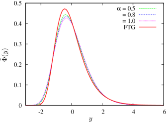
Figure 2: Numerically constructed MRH distributions for $\alpha=0.5,0.8$ and $1.0$ for system size $N=T/\tau=16384$. The FTG distribution is shown by the thick black line. Each distribution is rescaled to zero mean and unit standard deviation. It should be mentioned that the $\alpha<0.5$ curves are not displayed since they are indistinguishable from the $\alpha=0.5$ case.

However, in the case of i.i.d. random variables drawn from a Gaussian parent distribution (i.e. for $\alpha=0$), it has also been established that the convergence in $N$ towards the limiting FTG distribution is logarithmically slow Fisher and Tippett (1928); de Haan and Resnick (1996); Gomes and de Haan (1999). Therefore, in practice, the MRH distribution may appear different from FTG. An even worse rate of convergence may be expected with increasing $\alpha$, since, heuristically, increasing correlations decrease the effective number of degrees of freedom. In Fig. 2 we illustrate this trend by comparing numerical MRH distributions for a range of $\alpha$ but fixed $N$ with the FTG limiting distribution. For $\alpha<0.5$ the numerical distributions are practically indistinguishable from the case $\alpha=0.5$. This figure serves as a warning when comparing real-world data with known extreme value distributions.

We note here that Eichner et al. Eichner et al. (2006) have recently investigated EVS for $\alpha=0.6$. Although they do not spell it out explicitly, their Figs. 2 and 3 do demonstrate that the convergence at $\alpha=0.6$ (Fig. 3) is slower than at $\alpha=0$ (Fig. 2), in agreement with our findings described above.

In order to shed more light on convergence rates towards limiting distributions, we have measured the skewness $\gamma_{1}=\kappa_{3}/\kappa_{2}^{3/2}$ where $\kappa_{n}$ is the $n$-th cumulant of the MRH distribution function. The results for a range of $\alpha$ and $N$ are displayed in Fig. 3. From this plot one can discern a number of remarkable features. First, in the range $0\leq\alpha<1$, we note that the measured skewnesses are far from the skewness of the FTG distribution (approximately $1.140\ldots$), even for the largest system size available. Second, for $\alpha=0$, we know theoretically that the convergence rate is logarithmically slow, but, somewhat surprisingly, this convergence rate appears to be shared for all $\alpha\leq 0.5$, after which convergence slows down markedly. Thus, the universality in the ultimate limiting distribution for $0\leq\alpha<1$ may not carry over to a universality in the finite-size corrections. Note that if we did not know the limit but would try to determine it from finite-N skewnesses, then for $\alpha\lesssim 1$ we would be wrong to conclude that the asymptotic value had nearly been reached.

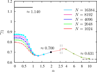
Figure 3: Strong finite-size effects at low values of $\alpha$ as seen in the scaled skewness, $\gamma_{1}=\kappa_{3}/\kappa_{2}^{3/2}$ of the MRH distribution. Note the exponential increasing system sizes $N=T/\tau$ used for comparisons. Note also that the scale of the horizontal axis changes at $\alpha=2.5$. The limiting value of $\gamma_{1}$ for $\alpha<1$ is $\gamma_{1}\approx 1.140$. Other exactly known values are $\gamma_{1}(\alpha=2)\approx 0.700$ and $\gamma_{1}(\alpha\to\infty)\approx 0.631$.

The case of strong correlations is discussed in the following sections. Here, we just observe that the skewnesses for $\alpha>1$ rapidly collapse for different $N$, and that they are virtually indistinguishable from each other for $\alpha\gtrsim 1.5$. In this case we may be quite sure that the skewnesses have practically reached their limiting values, since they match their corresponding theoretical values for $\alpha=2$ and $\infty$ with high accuracy. As we shall argue in Section VIII, in contrast to the very slow convergence for $0\leq\alpha<1$, convergence rate improves as it becomes a power law for $\alpha>1$.

V Strong-correlation regime: Exact results for $\alpha=2$ and $\alpha=\infty$.

The $1\leq\alpha<\infty$ region is characterized by diverging mean-square fluctuations (see Eq. (8)). Since $\langle h_{m}\rangle\geq\sqrt{\langle w_{2}\rangle}$, this is also a range where the characteristic scale of $\langle h_{m}\rangle$ diverges with the size of the system at least as $\langle h_{m}\rangle\sim T^{(\alpha-1)/2}$. An important exact result in the strongly-correlated regime is related to the Brownian random walk ($\alpha=2$). Majumdar and Comtet Majumdar and Comtet (2004, 2005) have shown that $\langle h_{m}\rangle\sim\sqrt{T}$ and, furthermore, they calculated the MRH distribution using path-integral techniques as well as by making a mapping to the problem of the area distribution under a Brownian excursion Takacs (1991, 1995). The resulting distribution is known as the Airy distribution. Under scaling by the average ($x=h_{m}/\langle h_{m}\rangle$), the Airy distribution can be written as follows (note that slightly different scaling has been used in Majumdar and Comtet (2004, 2005))

$$\Phi(x)=\frac{8\sqrt{3}}{\sqrt{\pi}x^{10/3}}\sum_{n=1}^{\infty}e^{-v_{n}/x^{2}}v_{n}^{2/3}U(-5/6,4/3,v_{n}/x^{2})\,.$$ (17)

Here $U(a,b,z)$ is the confluent hypergeometric function and $v_{n}=(2/\pi)\cdot(2\alpha_{n}/3)^{3}$ is related to the $n$-th zero $-\alpha_{n}$ of the Airy function.

The small and large $x$ asymptotes of $\Phi(x)$ have also been calculated Majumdar and Comtet (2004, 2005) with the results

$$\Phi(x\to 0)\sim\frac{8\sqrt{3}v_{1}^{3/2}}{\sqrt{\pi}x^{5}}e^{-v_{1}/x^{2}}\,$$ (18)

and

$$\ln\Phi(x\to\infty)\sim{-3\pi x^{2}/4}\,.$$ (19)

It is noteworthy that the above asymptotes are quite close in functional form to those obtained for the width distribution of the Edwards-Wilkinson model Foltin et al. (1994).

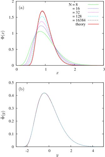
Figure 4: Convergence of the MRH distribution to its exactly known $N\to\infty$ limit Majumdar and Comtet (2004). Results for same system sizes are displayed in both panels using scaling by the average ($x=h_{m}/\langle h_{m}\rangle$) and $\sigma$-scaling [$y=(h_{m}-\langle h_{m}\rangle)/\sigma$] in the upper and lower panels, respectively. Very small system sizes were also displayed in order to demonstrate the remarkably fast convergence by $\sigma$-scaling.

The plot of $\Phi(x)$ is shown on Fig. 4a where a rather fast convergence to the limiting function can be seen (the convergence rate is $T^{-1/2}$ as calculated in Schehr and Majumdar (2006)). It is remarkable that the convergence is even faster if $\sigma$-scaling is used (Fig. 4b). The reason for this is the finite-size scaling of higher cumulants of the MRH distribution function. At this point we present this just as a numerical observation. A detailed study of the finite-size scaling of MRH will be published separately Györgyi et al. .

The review of the properties of the MRH distribution for $\alpha=2$ presented above gives a guidance for the discussion of EVS in the strong correlation regime. As we shall see below, the basic properties of EVS ($\langle h_{m}\rangle\sim\sqrt{\langle w_{2}\rangle}$, the general shape of $\Phi(x)$, the structure of the small- and large-$x$ asymptotics of $\Phi(x)$, the fast convergence to the limiting function) are similar in the whole $1<\alpha<\infty$ region.

The other analytically solvable case is the $\alpha\to\infty$ limit. Indeed, here only the $n=1$ mode survives, and the resulting signal $h(t)=|c_{1}|\sin{(2\pi t/T+\varphi)}$. Consequently, $h_{m}=|c_{1}|$ and the distribution of $h_{m}$ is just the distribution of $|c_{1}|$ given by $P(|c_{1}|)\sim|c_{1}|\exp{[-(2\pi)^{\alpha}T^{1-\alpha}|c_{1}|^{2}]}$. Using the average scaling, the scaling function $\Phi_{{}_{\infty}}(x)=\langle h_{m}\rangle P(\langle h_{m}\rangle x)$ becomes

$$\Phi_{{}_{\infty}}(x)=\frac{\pi}{2}x\theta(x)e^{-\pi x^{2}/4}\,.$$ (20)

were $\theta(x)$ is Heaviside’s step function. Comparing the above expression with the asymptotes (18) and (19), one can see that, in addition to the disappearance of the small $x$ singularity, the large $x$ asymptote has also changed by an extra $x$ factor.

VI The propagator of the generalized random acceleration process: $\alpha=2n$

The derivation of subsequent analytical results on the scale of $\langle h_{m}\rangle$, and on the small $h_{m}$ asymptote of the MRH distribution is based on the observation that $1/f^{\alpha}$ signals are actually paths of generalized random acceleration processes, provided that $\alpha=2n$ is an even integer. This allows a path-integral representation of the MRH distribution function (Sec. VII) from which rather general conclusions can be drawn and, furthermore, as indicated by the simulations, the results can be extended to any $1<\alpha<\infty$.

The construction of the MRH distribution function in the path integral approach involves the calculation of a normalization factor which, in turn, requires the knowledge of the propagator (also called two-time Green-function, or transition probability) of the random acceleration process. Here we compute this propagator, i.e. the probability density of a position of the stochastic path at some time $t$ conditioned on the initial point.

The equation of motion of the $1/f^{2n}$ trajectory reads

$$h^{[n]}(t)=\frac{\mathrm{d}^{n}h(t)}{\mathrm{d}t^{n}}=\xi(t),$$ (21)

where $\xi(t)$ is white noise with zero mean and correlation $\left\langle\xi(t)\xi(t^{\prime})\right\rangle=\delta(t-t^{\prime})$. Note that $h(t)$ corresponds to the $n-1$-st integral of the Brownian random walk trajectory. Eq. (21) can be rewritten as a vector Langevin equation

$$\dot{z}_{1}=\xi(t),\ \ \dot{z}_{k}=z_{k-1},\ (k=2,3,\dots n),\ \ z_{n}=h.$$ (22)

For $n=1$ we have the usual random walk, for $n=2$ the random acceleration problem Burkhardt (1993), also extensively studied, while for higher $n$-s one can speak about the generalized random acceleration processes Majumdar and Bray (2001); Schwarz and Maimon (2001). We are interested in the conditional probability that after time $t$ the trajectory is at $\mbox{\boldmath$z$}=(z_{1},z_{2},\ldots,z_{n})$ provided it started from $\mbox{\boldmath$z$}^{0}$. In the following, we denote this propagator by $G_{n}(\mbox{\boldmath$z$}|\mbox{\boldmath$z$}^{0};t)$. Its subscript indicates the dimension of the vector arguments, and it obviously satisfies the recursion relation

$$G_{n}(\mbox{\boldmath$z$}|\mbox{\boldmath$z$}^{0};t)=\int\mathrm{d}z_{n+1}\,G_{n+1}(\mbox{\boldmath$z$}|\mbox{\boldmath$z$}^{0};t)$$ (23)

where the integration eliminates the dependence on $z_{n+1}^{0}$, too. The propagator has Dirac delta initial condition, $G_{n}(\mbox{\boldmath$z$}|\mbox{\boldmath$z$}^{0};0)=\delta^{(n)}(\mbox{\boldmath$z$}-\mbox{\boldmath$z$}^{0})$, and satisfies the Fokker-Planck equation, obtained in a standard way from the Langevin equation van Kampen (1992),

$$\partial_{t}G_{n} = -\hat{H}_{n}^{0}G_{n}$$ (24)

$$\hat{H}_{n}^{0} = -\frac{1}{2}\partial_{1}^{2}+\sum_{k=1}^{n-1}z_{k}\partial_{k+1},$$ (25)

where $\partial_{t}$ and $\partial_{k}$ are derivatives with respect to $t$ and $z_{k}$, respectively. The superscript of $\hat{H}_{n}^{0}$ refers to the fact that we consider here the time evolution (21) without further constraints. The propagator has been calculated in previous studies up to $n=5$ Chaichian and Demichev (2001); Schwarz and Maimon (2001). We make an ansatz that matches these functions and we show it to be valid for general $n$

$$G_{n}(\mbox{\boldmath$z$}|\mbox{\boldmath$z$}^{0};t)=\prod_{k=1}^{n}\,\mathcal{G}(\mbox{\boldmath$a$}^{k}\!\!\cdot\!\mbox{\boldmath$z$}-\mbox{\boldmath$a$}^{0,k}\!\!\cdot\!\mbox{\boldmath$z$}^{0};\sigma_{k}),$$ (26)

where $\mathcal{G}(z;\sigma)=\exp{(-z^{2}/2\sigma^{2})}/\sqrt{2\pi}\sigma$ is a Gaussian PDF with zero mean and variance $\sigma^{2}$, $\mbox{\boldmath$z$}^{0}$ is the initial condition vector, and the vector $\mbox{\boldmath$a$}^{k}$ only has nonzero components for $i=1,2,\dots,k$, i.e., for $l>k$ we have $a_{l}^{k}=0$. In order to remove ambiguity we set $a_{k}^{k}=1$. The $\mbox{\boldmath$a$}^{k},\mbox{\boldmath$a$}^{0,k},\sigma_{k}$ are time dependent quantities to be determined. The above formula amounts to the recursion relation

$$G_{n}(\mbox{\boldmath$z$}|\mbox{\boldmath$z$}^{0};t) = G_{n-1}(\mbox{\boldmath$z$}|\mbox{\boldmath$z$}^{0};t)$$ (27)

$$\times\,\mathcal{G}(\mbox{\boldmath$a$}^{n}\!\!\cdot\!\mbox{\boldmath$z$}-\mbox{\boldmath$a$}^{0,n}\!\!\cdot\!\mbox{\boldmath$z$}^{0};\sigma_{n}).$$

Substitution of this ansatz into (24) leads to equations for the unknown parameters. The solution of the equations as described in Appendix A yields

$$a_{k}^{n}\,\, = \frac{(-t)^{n-k}(n+k-2)!}{2^{n-1}(2n-3)!!(k-1)!(n-k)!},$$ (28a)

$$a_{k}^{0,n} = (-1)^{n-k}a_{k}^{n},$$ (28b)

$$\sigma_{n}\,\, = \frac{t^{(2n-1)/2}}{2^{n-1}\sqrt{2n-1}(2n-3)!!}\,.$$ (28c)

For illustration, we use the above expressions to calculate and display explicitly the $n=4$ propagator. Noting that the original coordinate, velocity, acceleration, and its time derivative are given by

$$h=z_{4},\ \ v=z_{3},\ \ a=z_{2},\ \ \dot{a}=z_{1},$$ (29)

respectively, the propagator can be written in the form

$$G_{4}(\mbox{\boldmath$z$}|\mbox{\boldmath$z$}^{0};t)=\frac{720\sqrt{105}}{\pi^{2}t^{8}}e^{-A/2},$$ (30)

where $-A/2$ is the sum of the exponents of the Gaussians in (26), namely

$$A=\sum_{k=1}^{4}A_{k},$$ (31)

with

$$A_{1} = \frac{1}{t}(z_{1}-z_{1}^{0})^{2},$$ (32a)

$$A_{2} = \frac{12}{t^{3}}\left[z_{2}-z_{2}^{0}-\frac{t}{2}(z_{1}+z_{1}^{0})\right]^{2},$$ (32b)

$$A_{3} = \frac{720}{t^{5}}\left[z_{3}-z_{3}^{0}-\frac{t}{2}(z_{2}+z_{2}^{0})+\frac{t^{2}}{12}(z_{1}-z_{1}^{0})\right]^{2},$$ (32c)

$$A_{4} = \frac{100800}{t^{7}}\left[z_{4}-z_{4}^{0}-\frac{t}{2}(z_{3}+z_{3}^{0})+\frac{t^{2}}{10}(z_{2}-z_{2}^{0})\right.,$$ (32d)

$$\left.-\frac{t^{3}}{120}(z_{1}+z_{1}^{0})\right]^{2}.$$

Up to the $k=3$ term this incorporates the propagators of the random walk, $k=1$, random acceleration, $k\leq 2$, and random velocity of acceleration, $k\leq 3$, and the above expressions are in agreement with previous results Schwarz and Maimon (2001). Note that, independently of $k$ we have $a_{k}^{k}=a^{0,k}_{k}=1$, and

$$a^{k}_{k-1}=-a^{0,k}_{k-1}=t/2,$$ (33)

but for $l\leq k-2$ the $a_{l}^{k}$-s will vary with both $l$ and $k$.

Later, for the construction of the formula for the MRH distribution, we will need a special property of the propagator. Namely, if we consider the propagator of a periodic path of length $T$ and integrate it over the common values of the velocity, acceleration, etc., at the endpoints, we get the surprisingly simple result

$$\int\prod_{k=1}^{n-1}\mathrm{d}z_{k}^{0}\,G_{n}(\mbox{\boldmath$z$}^{0}|\mbox{\boldmath$z$}^{0};T)=T^{-(n-1/2)}(2\pi)^{-1/2}.$$ (34)

Indeed, the periodic propagator does not depend on $z_{n}^{0}$, the integration over $z_{n-1}^{0}$ cancels the normalizing constant of the $n$-th Gaussian but brings in a factor of $1/T$. The integration over $z_{n-2}^{0}$ does the same with the $n-1$-st Gaussian, and so on, until finally we are left with the norm factor of the $n=1$ Gaussian, $1/\sqrt{2\pi T}$, divided by $T^{n-1}$, as shown in (34). The key to this remarkable cancellation of the total numeric prefactor of the propagator is that (33) holds uniformly for all $k$-s.

VII Path integral formalism and the trace formula for the MRH ($\alpha=2n$)

For $\alpha=2$ Majumdar and Comtet Majumdar and Comtet (2004, 2005) introduced a path integral representation of the MRH distribution. The technique allowed for the formulation of the PDF in terms of the spectrum of a quantum mechanical, one-dimensional, Hamiltonian $\hat{H}$ with a hard wall and elsewhere linear potential, through the trace of $e^{-\hat{H}T}$, valid in the case of periodic boundary conditions. The spectrum is known to consist of the Airy zeros, so the trace formula resulted in the PDF called the Airy distribution.

In what follows we show that, in the case of periodic boundary conditions, for a general $\alpha=2n$, $n=2,3,\dots$ an analogous trace formula holds. Remarkably, the formula turns out to be essentially the same as in the $\alpha=2$ case, with the only difference that now a generalized “Hamiltonian” $\hat{H}_{n}$ appears. However, the $\hat{H}_{n}$, a differential operator in an $n$ dimensional space, is no longer Hermitian. Whereas we shall not solve the spectral problem necessary for the calculation of the MRH distribution, this formulation will allow us to (i) determine the scale of the MRH as function of $T$, and (ii) give explicitly the initial asymptote of the PDF, with the only undetermined parameter being the ground state energy of the Hamiltonian $\hat{H}_{n}$. What is more, the results (i-ii) will lend themselves to a continuation to real $\alpha$-s, so the use of the path integral technique extends beyond its original region of validity, the generalized random acceleration problem $\alpha=2n$.

We begin with the probability functional of a periodic path $h(t)$, where $h$ is measured from the time average,

$$P[h(t)] = \mathcal{A}\exp\left(-\frac{1}{2}\int_{0}^{T}\mathrm{d}t\,[h^{[n]}(t)]^{2}\right)$$ (35)

$$\times\delta\left(\int_{0}^{T}\mathrm{d}t\,h(t)\right).$$

Following Majumdar and Comtet (2004, 2005) we have introduced a normalizing coefficient $\mathcal{A}$, ensuring

$$\int_{\text{PBC}}\mathcal{D}_{n}h(t)P[h(t)]=1,$$ (36)

where PBC indicates that periodic boundary conditions for all derivatives of the path up to $h^{[n-1]}$ is understood. The measure $\mathcal{D}_{n}h(t)$ is defined such that the propagator $G_{n}(\mbox{\boldmath$z$}|\mbox{\boldmath$z$}^{0};T)$ of Sec. VI is a path integral without extra normalization, and the boundary conditions of the integral are specified by the arguments of $G_{n}$, i.e.

$$G_{n}(\mbox{\boldmath$z$}|\mbox{\boldmath$z$}^{0};T)=\int\mathcal{D}_{n}h(t)\exp\left(-\frac{1}{2}\int_{0}^{T}\mathrm{d}t\,[h^{[n]}(t)]^{2}\right)\!,\,$$ (37)

with $h^{[n-k]}(0)=z_{k}^{0},\,h^{[n-k]}(T)=z_{k}$, where $k=1,\dots n$. This $\mathcal{D}_{n}h(t)$ is in fact the measure leading naturally to the quantum-mechanical-like operator representation of the path integral

$$G_{n}(\mbox{\boldmath$z$}|\mbox{\boldmath$z$}^{0};T)=\left\langle\mbox{\boldmath$z$}|e^{-\hat{H}_{n}^{0}T}|\mbox{\boldmath$z$}^{0}\right\rangle,$$ (38)

where $\hat{H}_{n}^{0}$ is given by Eq. (25), and $\left|\mbox{\boldmath$z$}^{0}\right\rangle(\left\langle\mbox{\boldmath$z$}\right|$) are its right (left) eigenvectors corresponding to the $n$ dimensional positions indicated therein. Note that since this Hamiltonian is non-Hermitian for $n\geq 2$, the left and right eigenfunctions are different in general.

A third version of the propagator we shall utilize comes from a path integral by a measure of one order lower as

$$G_{n+1}(\mbox{\boldmath$z$}|\mbox{\boldmath$z$}^{0};T) = \int\mathcal{D}_{n}h(t)\exp\left(-\frac{1}{2}\int_{0}^{T}\mathrm{d}t\,[h^{[n]}(t)]^{2}\right)$$ (39)

$$\times\delta\left(z_{n+1}-\int_{0}^{T}h(t)\mathrm{d}t-z_{n+1}^{0}\right).$$

Here the Dirac delta produces the normalized density for the added area variable $z_{n}+1$. Note that if we take into account Eq. (37) then the consistency relation (23) immediately follows.

In order to determine the normalization coefficient $\mathcal{A}$ in (35), we express the equal-points propagator complemented with the area variable set to zero at both ends. By integrating over the path except for a single point and using Eqs. (35) and (39)

$$P_{\text{P}BC}(\mbox{\boldmath$z$}^{0}) = \int_{\text{PBC}:\mbox{\scriptsize\boldmath$z$}^{0}}\mathcal{D}_{n}h(t)P[h(t)]$$ (40)

$$= \mathcal{A}G_{n+1}(\mbox{\boldmath$z$}^{0},0|\mbox{\boldmath$z$}^{0},0;T).$$

where the mark PBC:$\mbox{\boldmath$z$}^{0}$ refers to the time derivatives at the ends fixed at $h^{[k]}(0)=h^{[k]}(T)=z_{n-k}^{0},\,k=0,\dots,n-1$. The $P_{\text{P}BC}(\mbox{\boldmath$z$}^{0})$ is the joint probability density of $h^{[k]}(t)=z_{n-k}^{0}$-s in a periodic path at any fixed time $t$, so as a byproduct we obtained that density in terms of the propagator, explicitly given in Sec. VI. That joint probability density is obviously normalized to unity. However, we know from Eq. (34) that the integral of the r.h.s. is independent of the $z_{n+1}^{0}$-st variable, and therefore we have

$$\mathcal{A}=T^{n+\frac{1}{2}}\sqrt{2\pi}.$$ (41)

For $n=1$ the normalizing coefficient derived in Majumdar and Comtet (2004, 2005) is recovered.

The integrated distribution $M(h_{\text{m}};T)$ of the MRH, i.e., the probability that the maximum does not exceed $h_{\text{m}}$, has been formulated in terms of a path integral in Majumdar and Comtet (2004, 2005). That expression is valid for any path density $P[h(t)]$ and reads formally as

$$M(h_{\text{m}};T) = \int_{-\infty}^{h_{\text{m}}}\mathrm{d}h\,P(h;T)$$ (42)

$$= \int_{\text{PBC}}\mathcal{D}h(t)P[h(t)]\prod_{t}\theta(h_{\text{m}}-h(t)).$$

Note that here $P(h_{\text{m}};T)$ is the density of MRH. Changing the integration variable and then introducing the hard wall potential $V_{0}(h)=\infty$ for $h<0$ and $V_{0}(h)=0$ for $h>0$, one obtains

$$M(h_{\text{m}};T) = \int_{\text{PBC}}\mathcal{D}h(t)P[h_{\text{m}}-h(t)]\prod_{t}\theta(h(t))$$ (43)

$$= \int_{\text{PBC}}\mathcal{D}h(t)P[h_{\text{m}}-h(t)]e^{-\int_{0}^{T}\mathrm{d}t\,V_{0}(h(t))}.$$

Using the specific form (35) of the probability functional we find

$$M(h_{\text{m}};T) = \mathcal{A}\int_{\text{PBC}}\mathcal{D}h(t)\,\delta\left(h_{\text{m}}T-\int_{0}^{T}\mathrm{d}t\,h(t)\right)$$ (44)

$$\times \exp\left[-\int_{0}^{T}\mathrm{d}t\,\left\{\frac{1}{2}(h^{[n]})^{2}+V_{0}(h(t))\right\}\right].$$

Next, we introduce the scaled Laplace transform of the integrated MRH distribution

$$K(u;T) = T\int_{0}^{\infty}\mathrm{d}h_{\text{m}}e^{-uh_{\text{m}}T}M(h_{\text{m}};T)$$ (45)

$$= \mathcal{A}\int_{\text{PBC}}\mathcal{D}h(t)$$

$$\times \exp\left[-\int_{0}^{T}\mathrm{d}t\,\left\{\frac{1}{2}(h^{[n]})^{2}+uV(h(t))\right\}\right],$$

where the potential $V(h)=\infty$ for $h<0$ and $V(h)=h$ for $h>0$.

In order to find $K(u;T)$, we write down the evolution equation for the PDF of the position and its derivatives $P_{n}(\mbox{\boldmath$z$};t)$ corresponding to the above path probability

$$\partial_{t}P_{n} = -\hat{H}_{n}(u)P_{n},$$ (46)

$$\hat{H}_{n}(u) = \hat{H}_{n}^{0}+uV(z_{n}),$$ (47)

where $\hat{H}_{n}^{0}$ was given in (25) and the variables $z_{k}$ are defined by (22). Thus the Laplace transform can be written in short as

$$K(u;T)=\mathcal{A}\,\text{Tr}\exp\left(-\hat{H}_{n}(u)T\right).$$ (48)

It is straightforward to show that the eigenvalues $E_{n,\omega}(u)$ of $\hat{H}_{n}(u)$, where $\omega$ summarizes all discrete indices, obey a simple scaling in $u$. For that purpose, let us consider the eigenvalue problem for $h=z_{n}>0$

$$\hat{H}_{n}(u)\psi=\left[-\frac{1}{2}\partial_{1}^{2}+\sum_{k=1}^{n-1}z_{k}\partial_{k+1}+uz_{n}\right]\psi=E_{n}(u)\psi$$ (49)

and apply a scale transformation by substituting

$$u^{\beta_{k}}z_{k}\to z_{k},\ \ \ u^{\delta}E_{n}\to E_{n}.$$ (50)

We recover an equation free of $u$, if all powers multiplying various terms are the same, that is

$$-2\beta_{1}=\beta_{1}-\beta_{2}=\dots=\beta_{n-1}-\beta_{n}=\beta_{n}+1=\delta,$$ (51)

so $\beta_{k}=(n-k+1)\delta-1$ and also $-2\beta_{1}=\delta$. Hence $\delta=\frac{2}{2n+1}$, so the eigenvalues scale like $E_{n,\omega}(u)=\epsilon_{n,\omega}u^{\frac{2}{2n+1}}$, where $\epsilon_{n,\omega}$ is the spectrum of $\hat{H}_{n}=\hat{H}_{n}(1)$.

It thus follows that, using (41), we get the scaling relation for the Laplace transform of the integrated distribution

$$K(u;T) = T^{n+\frac{1}{2}}{\cal K}(uT^{n+\frac{1}{2}})$$ (52)

$${\cal K}(s) = \sqrt{2\pi}\,\text{Tr}\exp\left(-\hat{H}_{n}s^{\frac{2}{2n+1}}\right)$$ (53)

$$= \sqrt{2\pi}\,\sum_{\omega}\exp\left(-\epsilon_{n,\omega}s^{\frac{2}{2n+1}}\right).$$

Hence, using (45), we obtain for the PDF of the MRH $P(h_{\text{m}};T)$ and its moment generating function $G(u;T)$ in scaling forms

$$P(h_{\text{m}};T) = \partial_{h_{\text{m}}}M(h_{\text{m}};T)=T^{\frac{1}{2}-n}P(h_{\text{m}}T^{\frac{1}{2}-n}),$$ (54)

$$G(v;T) = \int_{0}^{\infty}\mathrm{d}h_{\text{m}}\,P(h_{\text{m}};T)e^{-vh_{\text{m}}}=G(vT^{n-\frac{1}{2}}),\phantom{xx}$$ (55)

where

$$G(s) = \int_{0}^{\infty}\mathrm{d}z\,P(z)e^{-sz}$$ (56)

$$= s\,{\cal K}(s)$$

$$= \sqrt{2\pi}\,s\,\text{Tr}\exp\left(-\hat{H}_{n}s^{\frac{2}{2n+1}}\right)$$

$$= \sqrt{2\pi}\,s\,\sum_{\omega}\exp\left(-\epsilon_{n,\omega}s^{\frac{2}{2n+1}}\right).$$

Note that the same symbols $P,G$ are used for single- and double-argument functions, but that should not cause confusion. Remarkably, the trace formula is exactly the same as in the case of the simple random walk $n=1$, with the Hamiltonian $\hat{H}_{1}$ replaced by $\hat{H}_{n}$. Note that, in the special case of $n=1$, the scaling function of the MRH distribution (17) is ultimately recovered from the above trace formula Majumdar and Comtet (2005).

The scaled moment generating function Eq. (56) together with the preceding scaling formulas are our main result here. In the next two sections, we shall exploit the above results to draw conclusions about the scale and the small argument asymptote of the MRH distribution function.

VIII Strong-correlation regime ($1<\alpha<\infty$)

In order to evaluate the trace formula one would need the energy eigenvalues of $\hat{H}_{n}(1)$. Although they are known Majumdar and Comtet (2004) only for $n=1$, assuming that these eigenvalues exist, the scale of the MRH in $T$ can be derived since Eq. (54) yields

$$\langle h_{m}\rangle\sim T^{\,n-\frac{1}{2}}\quad.$$ (57)

As one can see, the scale of $\langle h_{m}\rangle$ is the same as that of the square root of the roughness Antal et al. (2002), i.e. we have $\langle h_{m}\rangle\sim\sqrt{\langle w_{2}\rangle}$ just as in the case of random walks Majumdar and Comtet (2004). It should be emphasized that while the above reasoning holds strictly for $\alpha=2n$, the exponent can, in fact, be continued naturally to real values. Thus it is plausible to surmise that $T^{\frac{\alpha-1}{2}}$ is the scale of the MRH for any $\alpha>1$. This power emerges quite sharply for $\alpha=1.3,1.6,2,4$ in numerical simulations as shown on the first panel of Fig. 5.

Fig. 5 also displays the 2nd and 3rd cumulants of $P(h_{m},T)$. We can observe the emergence of well defined scaling with $T$

$$\kappa_{k}(\alpha)\sim T^{k(\alpha-1)/2}\quad.$$ (58)

The scaling exponents are again equal to those of the cumulants of the width-distribution provided the $h_{m}\sim\sqrt{w_{2}}$ correspondence is used. This suggest that there is an intimate connection between the fluctuations of MRH and those of the signal width.

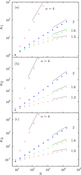
Figure 5: Cumulants, $\kappa_{k}$, of the MRH distribution for various $\alpha>1$ showing that $\kappa_{k}(\alpha)$ scales with system size, $N=T/\tau$, as $\kappa_{k}(\alpha)\sim N^{k(\alpha-1)/2}$. The straight lines have the appropriate asymptotic slopes $k(\alpha-1)/2$.

In order to see how the general shape changes as $\alpha$ is increased, we have performed simulations as described in Sec. III. The results are shown in Fig. 6 where we used scaling by the average to present the scaling functions $\Phi_{\alpha}(x)$.

The main features can be readily seen. The scaling function is a unimodal (single peaked) function which spreads out as $\alpha$ increases and approaches its $\alpha\to\infty$ limit (see Eq. (20)) rather fast. This is not entirely surprising since a glance at Fig. 1 convinces one that the $\alpha=10$ signal already consists of a single mode for all practical purposes, and thus the MRH distribution will be very well approximated by the $\Phi_{\infty}(x)$ function.

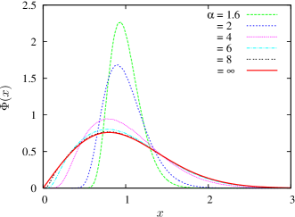
Figure 6: Numerically constructed MRH distributions for various $1<\alpha<\infty$. The $\alpha=\infty$ curve is the analytic result given in Eq. (20). System sizes $N\leq 16384$ were sufficiently large to observe the convergence of the PDF-s within the width of the lines drawn. Note that the $\alpha=8$ results are almost indistinguishable form the $\alpha\to\infty$ limit.

The function decays to zero extremly fast in the $x\to 0$ limit. The nonanalytical behavior and the actual functional form at small $x$ will be the subject of the next Section. Here, we call the reader’s attention to the fact that the region where the nonanalytic asymptotic behavior dominates is shrinking as $\alpha$ increases and, according to Eq. (20), entirely disappears in the $\alpha\to\infty$ limit.

The large $x$ limit is harder to treat analytically and we have only numerical evidence (Fig. 7) that the asymptotic behavior for large $x$ is given by

$$\Phi(x)\sim Cx^{\gamma}e^{-Bx^{2}}$$ (59)

where the parameters $B$, $C$, and $\gamma$ depend on $\alpha$. The above functional form is consistent with the exact result at $\alpha=\infty$ (see Eq. (20)). At $\alpha=2$, the ansatz of a Gaussian decay was shown to be in agreement Majumdar and Comtet (2004) with the large-order moments of the distribution function. However, the possibility of a prefactor $x^{\gamma}$ was not excluded by the analysis. We found that the generalized asymptote (59) with $\gamma\approx 2$ gives a superior fit to the large-$x$ ($x>1.5$) behavior of the exactly known PDF.

We have also fitted our numerical data in the region $x>1.5$ for larger $\alpha$-s, resulting in $\gamma\approx 1.4$ and $\gamma\approx 1.1$ for $\alpha=3$ and $4$, respectively. The general trend of the exponent $\gamma$ with increasing $\alpha$ is consistent with the $\alpha\to\infty$ limit of $\gamma_{\infty}=1$.

IX Initial asymptote

The trace formula (56) allows us to perform an asymptotic analysis of the MRH distribution for small arguments. The calculation is based on the large $s$ behavior of the moment generating function (56), wherein we assume that there is a positive, $\alpha=2n$-dependent, nondegenerate ground state energy $\epsilon_{0}(\alpha)$, which gives the leading term of the sum (while $\alpha$ is strictly even, several results will lend themselves to continuation). Under this assumption, the PDF in the scaled variable $z=h_{\text{m}}T^{\frac{1-\alpha}{2}}$ is asymptotically given by

$$P(z) = \int\frac{\mathrm{d}s}{2\pi i}G(s)e^{sz}$$ (60)

$$\approx \int\frac{\mathrm{d}s}{2\pi i}s\sqrt{2\pi}\,\exp\left(sz-\epsilon_{0}s^{\frac{2}{\alpha+1}}\right).$$

The above integral can be calculated using the saddle point method. For small $z$, the saddle point of the exponent is located on the real axis at

$$s^{\ast}\approx\left(\frac{2\epsilon_{0}}{(\alpha+1)z}\right)^{\frac{\alpha+1}{\alpha-1}}$$ (61)

and the integral in the neighborhood of the saddle point reduces to evaluating a Gaussian integral which yields the following asymptote

$$P(z) \approx Cz^{-\gamma}\exp\left(-B/z^{\beta}\right),$$ (62)

where the parameters are given by

$$\beta = \frac{2}{\alpha-1},$$ (63a)

$$\gamma = \frac{2\alpha+1}{\alpha-1},$$ (63b)

$$B = \frac{\alpha-1}{2}\left(\frac{2\epsilon_{0}}{\alpha+1}\right)^{\frac{\alpha+1}{\alpha-1}}$$ (63c)

$$C = \sqrt{\frac{\alpha+1}{\alpha-1}}\left(\frac{2\epsilon_{0}}{\alpha+1}\right)^{\frac{3}{2}\frac{\alpha+1}{\alpha-1}}.$$ (63d)

One should note that the exponents $\beta$ and $\gamma$ depend only on $\alpha$ while the amplitudes also depend on the ground state energy, $\epsilon_{0}(\alpha)$. The value of $\epsilon_{0}(\alpha)$ is known only for $\alpha=2$ where $\epsilon_{0}(2)=\alpha_{1}/\sqrt[3]{2}$, with $\alpha_{1}=2.3381$ being the absolute value of the first zero of the Airy function Majumdar and Comtet (2004, 2005).

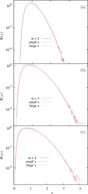
Figure 7: MRH distributions for (a): $\alpha=2$, (b): $\alpha=3$, and (c): $\alpha=4$, calculated for system size $N=16384$ (solid lines). The small and large $x$ asymptotes (dashed lines) are also shown. The small $x$ behavior in the range $0<x<1$ is fitted to the functional form (62) with the exponents $\beta,\gamma$ taken from (63). The prefactors $B,C$ are fitting parameters (note that the formulas in (63) contain an unkown parameter $\epsilon_{0}$). Large $x$ data in the range $x>1.5$ are fitted to the form (59), where $B$, $C$ and $\gamma$ are fitting parameters.

It should be emphasized that we did not scale the mean to $1$, being ignorant about the full PDF as well as its mean for general $\alpha$. So if comparing the above formula to the numerically scaled PDF as function of $x=z/\left\langle z\right\rangle$ then the factors $B,C$ will change and become fitting parameters. Figure 7 demonstrates the fit of (62) to simulation results for several $\alpha$-s, and we find that the fits are excellent in a surprisingly large interval. It should be noted that in the large $\alpha$ limit the initial slope is positive, so one expects a decreasing range of validity of the asymptote for increasing $\alpha$, nevertheless, the fit on Fig. 7 is quite good even for the largest $\alpha$. The case $\alpha=3$ demonstrates the continuation of the $\alpha=2n$ based formula, and suggests that naive continuation of at least the exponents $\beta,\gamma$ in (63) is justified.

Returning to the problem of scale-dependence of the amplitudes $B$ and $C$, we note that even if the full PDF is unknown, one can construct a parameter from the small-$x$ asymptote which does not depend on the scale. In order to see this, let us consider scaling by the average. With the rescaled variable $x$, one has the PDF as $\left\langle z\right\rangle P(x\left\langle z\right\rangle)$ and writing it again in the form (62) yields the following change of the amplitudes

$$B^{\prime}=\frac{B}{\left\langle z\right\rangle^{\beta}},\ \ \ C^{\prime}=\frac{C}{\left\langle z\right\rangle^{\gamma-1}}\,.$$ (64)

It follows from the above expressions that the following combination

$$D = \frac{B^{\frac{\alpha+2}{2}}}{C}=\frac{B^{\prime\frac{\alpha+2}{2}}}{C^{\prime}}$$ (65)

$$= \frac{(\alpha-1)^{\frac{\alpha+3}{2}}}{2^{\frac{\alpha+2}{2}}\sqrt{\alpha+1}}\left(\frac{2\epsilon_{0}}{\alpha+1}\right)^{\frac{\alpha+1}{2}}$$

remains independent of any scale change.

We should reiterate that the energy parameter $\epsilon_{0}(\alpha)$ is not known generally, but it is plausible to assume that it is a well defined number. It may be determined numerically for $\alpha=2n$ by a direct study of the corresponding local Hamiltonian. Remarkably, however, the above asymptotic formula allows for the computation of $\epsilon_{0}(\alpha)$ for any $\alpha>1$ from a numerical fit of the simulation result. Thus, precise MRH statistics effectively extract the ground state energy level of the Hamiltonian without solving the corresponding differential equation. Continuation of (62) for $\alpha\neq 2n$ is also natural here, but in this case we have a non-local Hamiltonian, whose spectral problem would be an even more challenging task to solve. Unfortunately, very high precision simulations are required to determine the ground state energy from the small-$x$ asymptote. In particular, our simulated data did not even allow the computation of the ground state energy to within a factor of 2 for the case of $\alpha=2$ where the lowest eigenvalue is known.

X MRH distribution for large $\alpha$

We have calculated the MRH distribution for the $\alpha\to\infty$ limit in Sec. V. There we found that only the $n=1$ mode survives and, as a result, the PDF (20) emerges. Here we discuss a procedure for perturbatively computing the leading corrections to (20) by taking into account the modes $n=2,3,\dots$.

First we reiterate that the amplitude of modes $c_{n}$ obey the distribution with action (3) and measure proportional to $\prod_{n}\theta(c_{n})c_{n}\mathrm{d}c_{n}$. Thus, separating the $n=1$ mode, the path in Fourier representation is written as

$$h(t)=a_{1}\sin(t)+\sum_{n=2}^{\infty}\varepsilon_{n}a_{n}\sin(nt+\varphi_{n}),$$ (66)

where the $\varepsilon_{n}=1/n^{\alpha/2}$ is the mean square root deviation of the amplitude of the $n$-th mode, and the $a_{n}=c_{n}/\varepsilon_{n}$-s are i.i.d. variables distributed according to

$$P_{0}(z)=2z\theta(z)\exp(-z^{2})\,.$$ (67)

Finally the phases $\varphi_{n}$ are independent and uniformly distributed in $[0,2\pi]$. The $n=0$ phase is omitted, because the choice of the origin is arbitrary. Obviously, $x$ measures the height from the time average of the path, which is here set to zero. Note that now time $t$ is in units of $2\pi/T$.

The leading correction from higher frequency modes can be calculated independently for each mode, thus here we only consider the $n$-th mode. Then the path is

$$h(t)=a_{1}\sin(t)+\varepsilon_{n}a_{n}\sin(nt+\varphi_{n})$$ (68)

and the calculation to leading order is straightforward. We compute the maximum of the path and then, knowing the distribution of all parameters therein, we can determine the PDF of the maximum. The details are presented in Appendix B, where we obtain the perturbed PDF for $h_{m}T^{\frac{1-\alpha}{2}}=z$ as

$$P(z)=P_{0}(z)+\varepsilon_{n}^{2}P_{2,n}(z)$$ (69)

with

$$P_{2,n}(z) = (1-n^{2}/2)\delta(z)+z\delta^{\prime}(z)/2$$ (70)

$$+e^{-z^{2}}\theta(z)\left(2z^{3}+(n^{2}-3)z\right).$$

The singular part needs some explanation here. As has been discussed in Sec. IX, for finite $\alpha$-s the PDF starts nonanalytically with zero initial slope for finite $\alpha$-s, in contrast to the $\alpha=\infty$ case, where the PDF has a finite slope. The nonanalyticity is not expected to be recovered by any expansion. Nonetheless, the formal expansion gives an explicit correction function $P_{2,n}$, with delta-singularity at the origin. It is plausible to conclude that while the expansion cannot be correct overall, the singularity “tries” to take care of the nonanalytic difference in the small-$z$ behavior, while the nonsingular part is expected to be a faithful correction for $z>0$. This leaves open the possibility that the large $\alpha$ expansion is not convergent, rather it is asymptotic.

Next we scale the PDF to unit average. Using the result (101) from Appendix B one finds

$$\Phi(x)=\Phi_{{}_{\infty}}(x)+\varepsilon_{n}^{2}\Phi_{2,n}(x)$$ (71)

where $\Phi_{{}_{\infty}}(x)$ is given in (20) and

$$\Phi_{2,n}(x) = (1-n^{2}/2)\delta(x)+x\delta^{\prime}(x)/2$$ (72)

$$+e^{-\pi x^{2}/4}\theta(x)\frac{\pi}{8}(n^{2}-1)\left(6x-\pi x^{3}\right).$$

Formally, we can sum up the leading corrections for all $n$-s. However, this is not a consistent approximation, because, for instance, $\varepsilon_{2}^{2}=\varepsilon_{4}$, so the leading correction from $n=4$ is of the same order as the quadratic one from $n=2$. Therefore we use the sum of the corrections for only $n=2,3$ to test the prediction. On Fig. 8 we display the correction

$$\Delta\Phi(x)=\Phi(x)-\Phi_{{}_{\infty}}(x)$$ (73)

of the PDF from simulation for a series of $\alpha$-s, together with the theoretical prediction for corrections added up from the modes $n=2,3$,

$$\Delta\Phi(x)\approx\varepsilon_{2}^{2}\Phi_{2,2}(x)+\varepsilon_{3}^{2}\Phi_{2,3}(x).$$ (74)

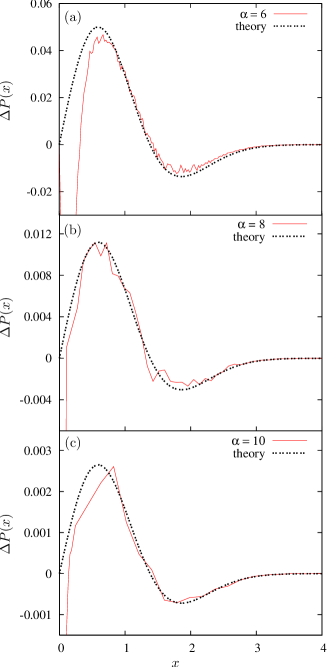
Figure 8: Difference $\Delta P(x)$ between the MRH distribution for large $\alpha$ and $\alpha=\infty$, as defined in (73). We also display the smooth part of the leading correction (74) from perturbation theory added up from the modes $n=2,3$.

It should be mentioned that the sum of leading corrections for all modes has a prefactor $\sum_{n=2}^{\infty}(n^{2}-1)\varepsilon_{n}^{2}=\zeta(\alpha-2)-\zeta(\alpha)$. This diverges for $\alpha\to 3^{+}$, so the series does not converge for $\alpha\leq\alpha_{c}=3$, which is the borderline for the differentiability of the path. We cannot exclude that higher order corrections, involving higher order differentiation of the path, further tighten the range of convergence.

XI Comparison with the roughness and the maximal intensity

Here we compare the statistical properties of $h_{m}$ to those of the roughness $w_{2}$, i.e. of the mean square deviation, or width of the trajectory (7). The latter was one of the first global quantities of stochastic signals whose scaling properties and statistics were extensively studied for $1/f^{\alpha}$ processes Antal et al. (2002).

One of the reasons for comparison is that both $\langle h_{m}\rangle$ and $\sqrt{\langle w_{2}\rangle}$ scale similarly with $T$ for $\alpha\geq 1$ and, furthermore, there are many common features at the level of their PDF-s. Namely, for algebraically diverging correlations, $\alpha>1$, after scaling by the mean, the PDF-s are nondegenerate (each cumulant is finite), that is, scaling by the mean is a natural representation of both PDF-s. As $\alpha\to 1$, the PDF-s scaled by the mean approach a Dirac-delta and, in the range $\alpha\leq 1$, they both lend themselves to scaling by the standard deviation. Here an important difference emerges. In the range $0.5<\alpha\leq 1$ the roughness has a nontrivial PDF while below the critical $\alpha=0.5$ it becomes trivial, i.e. the roughness becomes Gaussian distributed. On the other hand, the MRH has the trivial FTG limiting distribution in the entire $0<\alpha<1$ region. We can only speculate that the threshold near $\alpha=0.5$ manifests itself in the MRH distribution in its approach to the FTG limit, as suggested by the finite-size dependence of the simulation results shown in Fig. 3. This, however, is just a numerical observation without theoretical foundations as yet.

Further motivation for a closer comparison comes from the similarities in the shape of the two families of PDF-s in the $\alpha>1$ region. First, in the $\alpha\to\infty$ limit, the PDF-s are the same if the $h_{m}\sim\sqrt{w_{2}}$ correspondence is made. Second, for finite $\alpha$-s, the unimodal PDF-s have asymptotes which are similar for both small and large arguments. Specifically, there is a Gaussian decay at large $x$, while the small $x$ behavior is dominated by an exponential nonanalytic term with a power prefactor. Here, the comparisons can be made quantitatively for small $x$, since analytic results are available for general $\alpha$.

Last but not least, a reason for a closer comparison comes from the fact that the roughness can also be conceived as obeying an EVS. Bertin and Clusel Bertin (2005); Bertin and Clusel (2006) made the remarkable observation that since the roughness is essentially the integrated power spectrum, i.e., the sum of nonnegative Fourier intensities, it is in effect the maximum of positive partial sums. In general, the partial sums are correlated but, for the special case of $\alpha=1$, they correspond to the ordered sequence of i.i.d. variables. As a consequence, FTG distribution emerges for $w_{2}$ at $\alpha=1$, thus providing insight to an earlier rather puzzling result Antal et al. (2001) in connection with $1/f$ noise. It then becomes a rather interesting open question how the MRH distribution differs from the roughness distribution for $\alpha>1$ where the latter also describes the EVS of correlated variables.

The initial asymptote of the MRH distribution (62),(63) should be compared with that for the roughness distribution obtained in appendix E of Györgyi et al. (2003)

$$\Phi_{w}(x) \approx C_{w}x^{-\gamma_{w}}\exp\left(-B_{w}/x^{\beta_{w}}\right),$$ (75)

where the parameters are given by

$$\beta_{w} = \frac{1}{\alpha-1},$$ (76a)

$$\gamma_{w} = \frac{3\alpha-1}{2(\alpha-1)},$$ (76b)

$$B_{w} = (\alpha-1)\left(\frac{\pi}{\alpha\sin(\pi/\alpha)}\right)^{\frac{\alpha}{\alpha-1}}\zeta(\alpha)^{-\frac{1}{\alpha-1}}$$ (76c)

$$C_{w} = \frac{(2\pi)^{\frac{\alpha-1}{2}}}{\sqrt{\alpha-1}}\left(\frac{\pi}{\sin(\pi/\alpha)}\right)^{\frac{\alpha}{\alpha-1}}\left(\zeta(\alpha)\alpha\right)^{-\frac{\alpha+1}{2(\alpha-1)}}$$ (76d)

with $\zeta(\alpha)$ denoting the Riemann’s zeta function. Note that this asymptote does not contain unknown parameters such as $\epsilon_{0}$ in the MRH distribution.

Interestingly, comparison with the exponents in the asymptote of the MRH, (62), shows that the respective $\gamma$-s are the same, if $\sqrt{w_{2}}$ is considered, i.e., $2\gamma_{w}=\gamma$. Nevertheless, the respective exponents in the prefactor, $2\beta_{w}+1$ and $\beta$, agree only at an accidental $\alpha$ and are otherwise different.

The present results on the small-$x$ asymptote may also be compared to the asymptote of the distribution of the maximal Fourier intensity. It is defined as the maximal of the $|c_{n}|^{2}$ intensity components for a given realization of the path, which obeys some PDF if the ensemble of $1/f^{\alpha}$ paths is considered. This was to our knowledge the first quantity whose EVS was studied in the context of $1/f^{\alpha}$ signals Györgyi et al. (2003). Again, the overall shape of the PDF of the extremal intensity is similar to those of the MRH and the roughness: its initial part is suppressed nonanalytically and has a single maximum, before smoothly decaying for large arguments. There the critical $\alpha_{c}$ where the FTG limit distribution emerges is $\alpha_{c}=0$, in contrast to the MRH and the roughness, where this critical values are $\alpha_{c}=1$ and $\alpha_{c}=0.5$, respectively. As we have shown in Györgyi et al. (2003), written with $\alpha_{c}$, the powers in the asymptotic formula for the maximal intensity and for the roughness are the same

$$\beta_{w}=\beta_{\text{I}}=\frac{1}{\alpha-\alpha_{c}},\ \ \ \gamma_{w}=\gamma_{\text{I}}=\frac{3(\alpha-\alpha_{c})+2}{2(\alpha-\alpha_{c})},$$ (77)

where the exponents $\beta_{\text{I}},\gamma_{\text{I}}$ are defined in the same way for the initial asymptote of the PDF of the maximal intensity as $\beta_{w},\gamma_{w}$ were for the PDF of the roughness.

In conclusion, the respective PDF-s of the MRH, the maximal intensity, and the roughness are similarly looking, unimodal functions, with nonanalytically slow initial behavior. Despite the qualitative similarities, however, it is clear that the three PDF-s are quantitatively different. This is natural since they describe different physical quantities. One may, however, speculate that the similar features have their roots in the divergent correlations present in the $\alpha\geq 1$ region.

XII Final remarks

It should be emphasized that we are only at the first stages of understanding the effects of correlations on EVS. One of the important tasks for future studies should be the understanding of the convergence properties in the $0<\alpha<1$ range. Although the limit distribution is known here, the convergence is extremely slow. Since most of the environmental time series of general interest (data on temperature, precipitation, etc.) correspond to this range, as they exhibit generically correlations with power-type decay, and the length of the series is naturally restricted, the development of a theory of finite-size corrections is important. The much discussed $\alpha\to 1$ case is even more challenging since it appears to be outside the reach of present computing abilities. Thus new analytical approaches and ideas for numerical recipes are called for.

Another relevant problem is the question of boundary conditions. It is known from the $\alpha=2$ case, where both periodic and free boundary conditions were investigated Majumdar and Comtet (2004), that the MRH distribution depends on boundary conditions. Since the analysis of a real time series usually means cutting it up into smaller pieces and making statistics out of the properties of these subsequences, the appropriate boundary conditions in this case are the so-called window boundary conditions, when the window under consideration is embedded in a longer signal. These boundary conditions have been discussed in connection with the roughness distribution of $1/f^{\alpha}$ signals Antal et al. (2002). It has been found that the limit distributions depends on the window size (even in the limit of large external system) and furthermore, the effects become stronger as $\alpha$ increases. Clearly, similar studies should be carried out for the EVS problem.

Finally, it remains to be seen if the investigations of the effects of correlations, in particular the effects of strong correlations, will allow us a universal classification of EVS similar to that existing for thermodynamic critical points.

Appendix A Derivation of the propagator for $\alpha=2n$

Here we show that the ansatz (27) indeed satisfies the Fokker-Planck equation (25) with the coefficients (28). Let us start out from (25)

$$\partial_{t}G_{n}=\frac{1}{2}\partial_{1}^{2}G_{n}-\sum_{k=1}^{n-1}z_{k}\partial_{k+1}G_{n},$$ (78)

and substitute

$$G_{n}=G_{n-1}\mathcal{G},$$ (79)

where the arguments are understood as in (27). Using the fact that $G_{n-1}$ also satisfies (78), we arrive at

$$\partial_{t}\mathcal{G}=\frac{1}{2}\partial_{1}^{2}\mathcal{G}+\partial_{1}\mathcal{G}\,\partial_{1}\ln G_{n-1}-\sum_{k=1}^{n-1}z_{k}\partial_{k+1}\mathcal{G}.$$ (80)

From (27) we have

$$\partial_{k}\mathcal{G} = a_{k}^{n}\mathcal{G}^{\prime},$$ (81a)

$$\partial_{k}^{2}\mathcal{G} = (a_{k}^{n})^{2}\mathcal{G}^{\prime\prime},$$ (81b)

where, denoting $\mbox{\boldmath$a$}^{n}\!\!\cdot\!\mbox{\boldmath$z$}-\mbox{\boldmath$a$}^{0,n}\!\!\cdot\!\mbox{\boldmath$z$}^{0}$ by $x$,

$$\mathcal{G}^{\prime}(x;\sigma) = -\frac{x}{\sigma^{2}}\mathcal{G}(x;\sigma),$$ (82a)

$$\mathcal{G}^{\prime\prime}(x;\sigma) = -\frac{\mathcal{G}(x;\sigma)}{\sigma^{2}}-\frac{x}{\sigma^{2}}\mathcal{G}^{\prime}(x;\sigma),$$ (82b)

and, furthermore, using the full exponent of the ansatz (26) we have

$$\partial_{1}\ln G_{n-1}=-\sum_{k=1}^{n-1}\frac{a_{1}^{k}}{\sigma^{2}_{k}}(\mbox{\boldmath$a$}^{k}\!\!\cdot\!\mbox{\boldmath$z$}-\mbox{\boldmath$a$}^{0,k}\!\!\cdot\!\mbox{\boldmath$z$}^{0}).$$ (83)

Differentiation of the Gaussian $\mathcal{G}$ by time gives

$$\partial_{t}\mathcal{G} = -\frac{1}{2}\frac{\dot{\sigma^{2}_{n}}}{\sigma^{2}_{n}}\mathcal{G}-\frac{1}{2}\frac{\dot{\sigma^{2}_{n}}}{\sigma^{2}_{n}}(\mbox{\boldmath$a$}^{n}\!\!\cdot\!\mbox{\boldmath$z$}-\mbox{\boldmath$a$}^{0,n}\!\!\cdot\!\mbox{\boldmath$z$}^{0})\mathcal{G}^{\prime}$$ (84)

$$+(\dot{}\mbox{\boldmath$a$}^{n}\!\!\cdot\!\mbox{\boldmath$z$}-\dot{}\mbox{\boldmath$a$}^{0,n}\!\!\cdot\!\mbox{\boldmath$z$}^{0})\mathcal{G}^{\prime},$$

where we have condensed some $z$ dependence by factoring out $\mathcal{G}^{\prime}$. On the other hand, according to Eqs. (81),(82), the r.h.s. of (80) yields

$$\partial_{t}\mathcal{G} = -\frac{1}{2}(a_{1}^{n})^{2}\left(\frac{\mathcal{G}}{\sigma^{2}_{n}}+\frac{\mbox{\boldmath$a$}^{n}\!\!\cdot\!\mbox{\boldmath$z$}-\mbox{\boldmath$a$}^{0,n}\!\!\cdot\!\mbox{\boldmath$z$}^{0}}{\sigma^{2}_{n}}\mathcal{G}^{\prime}\right)$$ (85)

$$-a_{1}^{n}\mathcal{G}^{\prime}\sum_{k=1}^{n-1}\frac{a_{1}^{k}}{\sigma^{2}_{k}}(\mbox{\boldmath$a$}^{k}\!\!\cdot\!\mbox{\boldmath$z$}-\mbox{\boldmath$a$}^{0,k}\!\!\cdot\!\mbox{\boldmath$z$}^{0})$$

$$-\sum_{k=1}^{n-1}z_{k}a^{n}_{k+1}\mathcal{G}^{\prime}.$$

Equating (84) with (85) should give the sought after equations for $\mbox{\boldmath$a$},\mbox{\boldmath$a$}^{0},\sigma$. Comparing the $z$-independent factors of $\mathcal{G}$ in (84) and in (85) gives

$$\dot{\sigma^{2}_{n}}=(a_{1}^{n})^{2}.$$ (86)

Thus the full first lines on the r.h.s. of (84) and (85) are equal. In the rest we change the summation variable $k$ to $l$ and then equate the respective factors of $z_{k}$ and those of $z_{k}^{0}$ to obtain differential equations for the coefficients

$$\dot{a}_{k}^{n} = -a_{1}^{n}\sum_{l=k}^{n-1}\frac{a_{1}^{l}a^{l}_{k}}{\sigma^{2}_{l}}-a_{k+1}^{n},$$ (87a)

$$\dot{a}_{k}^{0,n} = -a_{1}^{n}\sum_{l=k}^{n-1}\frac{a_{1}^{l}a_{k}^{0,l}}{\sigma^{2}_{l}},$$ (87b)

where we have used the condition that $a^{l}_{k}=a^{0,l}_{k}=0$ for $k>l$. Next, we determine the time dependence of the $a$-s by assuming it to be power law and requiring that terms in each differential equation have the same power. Thus we separate the time dependence, and for later purposes also factorize the constants as

$$a_{k}^{n}=t^{n-k}b^{n}_{k}\,c_{n},\ \ \ a_{k}^{0,n}=t^{n-k}b^{0,n}_{k}\,c_{n},$$ (88)

for all nonnegative integers $n,k$. We also set $b_{k}^{n}=0$ for $n<k$ to ensure that $a_{k}^{n}$ vanishes for such indices. The $c_{n}$-s are made unambiguous by requiring $b_{1}^{n}=1$ and, furthermore, since $a^{n}_{n}=1$ thus $b^{n}_{n}=1/c_{n}$. Then (86) gives

$$\sigma^{2}_{n}=(c_{n})^{2}\frac{t^{2n-1}}{2n-1}.$$ (89)

The parameterization in (88) is justified by the fact that substituting it into (87) the $c$-s disappear, so what remains are equations for the $b$-s as

$$b_{k+1}^{n} = -(n-k)b_{k}^{n}-\sum_{l=k}^{n-1}(2l-1)b^{l}_{k}$$ (90a)

$$b_{k}^{0,n} = -\frac{1}{n-k}\sum_{l=k}^{n-1}(2l-1)b_{k}^{0,l}.$$ (90b)

For a few small integer indices these equations can be solved, whence the following general formulas can be surmised

$$b_{k}^{n} = (-1)^{k-1}\frac{(n+k-2)!}{(n-k)!(k-1)!},$$ (91a)

$$b_{k}^{0,n} = (-1)^{n-k}b_{k}^{n}.$$ (91b)

Note that Eqs. (90a) and (90b) are homogeneous linear equations leaving room for overall factors in the solution. They are set by the conditions (i) $b^{n}_{1}=1$ and (ii) $b^{0,n}_{n}=b^{n}_{n}$. Condition (i) was stated earlier below Eq. (88), while (ii) is equivalent to the requirement that $G_{n}$ depends on $z_{n}$ and $z_{n}^{0}$ only through their difference.

One can confirm proposition (91) by substituting it into (90) and then using the identities

$$\sum_{l=k}^{n-1}\!\frac{(2l-1)(k+l-2)!}{(l-k)!} \hskip 10.0pt=\!\!\frac{n-1}{k}\frac{(n+k-2)!}{(n-k-1)!},$$ (92a)

$$\sum_{l=k}^{n-1}(-1)^{l}\frac{(2l-1)(k+l-2)!}{(l-k)!}$$ (92b)

$$= (-1)^{n+1}\frac{(n+k-2)!}{(n-k-1)!},$$

which may be proved by induction.

Finally, with (91) together with

$$c_{n} = \frac{1}{b_{n}^{n}}=\frac{1}{(-2)^{n-1}(2n-3)!!}$$ (93)

we have all ingredients of (88) to calculate the $a$-s, the result being displayed in Eq. (28). The standard deviation $\sigma_{n}$ given in (28) follows then from (89) and (93).

Appendix B Leading perturbation of the PDF for large $\alpha$ from the $n$th mode

We start out from the Fourier representation (68) of the path with one mode of frequency $n$ beside the basic one ($n=1$). From the condition $h^{\prime}(t_{0})=0$, we obtain the correction in the position $t_{0}=\pi/2+\delta_{n}$ of the maximum to leading order

$$\delta_{n}=n\varepsilon_{n}\frac{a_{n}}{a_{1}}\cos\left(\frac{n\pi}{2}+\varphi_{n}\right).$$ (94)

Hence we can calculate the maximum to second order in $\varepsilon_{n}$ (the quadratic correction in $\delta_{n}$ contributes only to cubic order)

$$h_{\text{m}}=h(t_{0}) \approx h(\pi/2)+h^{\prime}(\pi/2)\delta_{n}+1/2h^{\prime\prime}(\pi/2)\delta_{n}^{2}$$ (95)

$$\approx a_{1}+\varepsilon_{n}a_{n}\sin\left(\frac{n\pi}{2}+\varphi_{n}\right)$$

$$+\frac{n^{2}\varepsilon_{n}^{2}a_{n}^{2}}{2a_{1}}\cos^{2}\left(\frac{n\pi}{2}+\varphi_{n}\right).$$

Now the PDF for the MRH $h_{\text{m}}$ is obtained by averaging over $a_{1},a_{n},\varphi_{n}$ in

$$P(z) = \left\langle\delta\left(z-h_{\text{m}}\right)\right\rangle\,.$$ (96)

Expanding to second order, one finds

$$P(z) = \left\langle\delta\left(z-a_{1}\right)\right\rangle-\left\langle\delta^{\prime}\left(z-a_{1}\right)\left[\varepsilon_{n}a_{n}\sin\left(\frac{n\pi}{2}+\varphi_{n}\right)\right.\right.$$ (97)

$$+\left.\left.\frac{n^{2}\varepsilon_{n}^{2}a_{n}^{2}}{2a_{1}}\cos^{2}\left(\frac{n\pi}{2}+\varphi_{n}\right)\right]\right\rangle$$

$$+\frac{\varepsilon_{n}^{2}}{2}\left\langle\delta^{\prime\prime}\left(z-a_{1}\right)a_{n}^{2}\sin^{2}\left(\frac{n\pi}{2}+\varphi_{n}\right)\right\rangle.$$

Note that here derivatives of the Dirac-delta appear. Now performing the averages yields ($P_{0}$ is given by Eq. (67))

$$P(z) = P_{0}(z)+\varepsilon_{n}^{2}P_{2,n}(z),$$ (98)

$$P_{2,n}(z) = -\frac{n^{2}}{2}\left(\theta(z)e^{-z^{2}}\right)^{\prime}+\frac{1}{2}\left(\theta(z)ze^{-z^{2}}\right)^{\prime\prime}.$$ (99)

Differentiation of the terms with step-functions gives

$$P_{2,n}(z) = (1-n^{2}/2)\delta(z)+z\delta^{\prime}(z)/2$$ (100)

$$+e^{-z^{2}}\theta(z)\left(2z^{3}+(n^{2}-3)z\right),$$

where the term proportional to $z^{2}\delta(z)$ has been omitted, since it does not contribute to the average and other moments of nonsingular functions. Hence we obtain formula (70).

The mean to second order is best calculated from (98),(99) resulting in

$$\left\langle z\right\rangle = \frac{\sqrt{\pi}}{2}+\varepsilon_{n}^{2}\frac{n^{2}\sqrt{\pi}}{4}.$$ (101)

The scaled PDF is then obtained by the change of variable from $z$ to $x=z/\left\langle z\right\rangle$, and expanding the resulting expression to second order in $\varepsilon_{n}$ yields Eqs. (71) and (72).

References

- Fisher and Tippett (1928) R. Fisher and L. Tippett, Procs. Cambridge Philos. Soc. 24, 180 (1928).
- Gnedenko (1943) B. Gnedenko, Ann. Math. 44, 423 (1943).
- Gumbel (1958) E. Gumbel, Statistics of Extremes (Dover Publications, 1958).
- Katz et al. (2002) R. W. Katz, M. B. Parlange, and P. Naveau, Adv. Water Resour. 25, 1287 (2002).
- v. Storch and Zwiers (2002) H. v. Storch and F. W. Zwiers, Statistical Analysis in Climate Research (Cambridge University Press, Cambridge, 2002).
- Gutenberg and Richter (1944) B. Gutenberg and C. F. Richter, Bull. Seismol. Soc. Am. 34, 185 (1944).
- Majumdar and Comtet (2004) S. Majumdar and A. Comtet, Phys. Rev. Lett. 92, 225501 (2004).
- Majumdar and Comtet (2005) S. Majumdar and A. Comtet, J. Stat. Phys. 119, 777 (2005).
- Antal et al. (2001) T. Antal, M. Droz, G. Györgyi, and Z. Rácz, Phys. Rev. Lett. 87, 240601 (2001).
- Györgyi et al. (2003) G. Györgyi, P. Holdsworth, B. Portelli, and Z. Rácz, Phys. Rev. E 68, 056116 (2003).
- Lee (2005) D.-S. Lee, Phys. Rev. Lett. 95, 150601 (2005).
- Bolech and Rosso (2004) C. Bolech and A. Rosso, Phys. Rev. Lett. 93, 125701 (2004).
- Bertin (2005) E. Bertin, Phys. Rev. Lett. 95, 170601 (2005).
- Guclu and Korniss (2004) H. Guclu and G. Korniss, Phys. Rev. E 69, 065104(R) (2004).
- Krapivsky and Majumdar (2000) P. Krapivsky and S. Majumdar, Phys. Rev. Lett. 84, 5492 (2000).
- Majumdar and Krapivsky (2002) S. Majumdar and P. Krapivsky, Phys. Rev. E 65, 036127 (2002).
- Bunde et al. (2005) A. Bunde, J. F. Eichner, J. W. Kantelhardt, and S. Havlin, Phys. Rev. Lett. 94, 048701 (2005).
- Király et al. (2006) A. Király, I. Bartos, and I. M. Jánosi, Tellus A 58A, 593 (2006).
- Yakimov and Hooge (2000) A. V. Yakimov and F. N. Hooge, Physica B 291, 97 (2000).
- Monetti et al. (2002) R. A. Monetti, S. Havlin, and A. Bunde, Physica A 320, 581 (2002).
- Blender et al. (2006) R. Blender, K. Fraedrich, and B. Hunt, Geophys. Res. Lett. 33, L04710 (2006).
- Lillo and Mantegna (2000) F. Lillo and R. N. Mantegna, Phys. Rev. E 62, 6126– (2000).
- Raychaudhuri et al. (2001) S. Raychaudhuri, M. Cranston, C. Przybyla, and Y. Shapir, Phys. Rev. Lett. 87, 136101 (2001).
- Galambos (1978) J. Galambos, The Asymptotic Theory of Extreme Value Statistics (John Wiley & Sons, 1978).
- de Haan and Ferreira (2006) L. de Haan and A. Ferreira, Extreme Value Theory: An Introduction (Springer, New York, 2006).
- Berman (1964) S. M. Berman, Ann. Math. Statist. 33, 502 (1964).
- Antal et al. (2002) T. Antal, M. Droz, G. Györgyi, and Z. Rácz, Phys. Rev. E 65, 046140 (2002).
- Weissman (1988) M. Weissman, Rev. Mod. Phys. 60, 537 (1988).
- Edwards and Wilkinson (1982) S. Edwards and D. Wilkinson, Philos. Trans. R. Soc. London A 381, 17 (1982).
- Mullins (1957) W. W. Mullins, J. Appl. Phys. 28, 333 (1957).
- Villain (1991) J. Villain, J. Phys. I France 1, 19 (1991).
- Burkhardt (1993) T. W. Burkhardt, J. Phys. A: Math. Gen. 26, L1157 (1993).
- Krug (1997) J. Krug, Adv. Phys. 46, 139 (1997).
- Barabási and Stanley (1995) A.-L. Barabási and H. Stanley, Fractal Concepts in Surface Growth (Cambridge University Press, Cambridge, 1995).
- Foltin et al. (1994) G. Foltin, K. Oerding, Z. Rácz, R. Workman, and R. Zia, Phys. Rev. E 50, R639 (1994).
- de Haan and Resnick (1996) L. de Haan and S. Resnick, Annals of Probability 24, 97 (1996).
- Gomes and de Haan (1999) M. I. Gomes and L. de Haan, Extremes 2, 71 (1999).
- Eichner et al. (2006) J. F. Eichner, J. W. Kantelhardt, A. Bunde, and S. Havlin, Phys. Rev. E 73, 016130 (2006).
- Takacs (1991) L. Takacs, Adv. Appl. Prob. 23, 557 (1991).
- Takacs (1995) L. Takacs, J. Appl. Prob. 32, 375 (1995).
- Schehr and Majumdar (2006) G. Schehr and S. N. Majumdar, Phys. Rev. E 73, 056103 (2006).
- (42) G. Györgyi, N. R. Moloney, K. Ozogány, and Z. Rácz, to be published.
- Majumdar and Bray (2001) S. Majumdar and A. J. Bray, Phys. Rev. Lett. 86, 3700 (2001).
- Schwarz and Maimon (2001) J. Schwarz and R. Maimon, Phys. Rev. E 64, 016120 (2001).
- van Kampen (1992) N. G. van Kampen, Stochastic Processes in Physics and Chemistry (North Holland, Amsterdam, 1992).
- Chaichian and Demichev (2001) M. Chaichian and A. Demichev, Path Integrals in Physics, vol. 1 (Institute of Physics Publishing, Bristol, 2001).
- Bertin and Clusel (2006) E. Bertin and M. Clusel, J. Phys. A: Math. Gen. 39, 7607 (2006).