Dispersion and transitions of dipolar plasmon modes in graded plasmonic waveguides

Abstract

Coupled plasmon modes are studied in graded plasmonic waveguides, which are periodic chains of metallic nanoparticles embedded in a host with gradually varying refractive indices. We identify three types of localized modes called “light”, “heavy”, and “light-heavy” plasmonic gradons outside the passband, according to various localization. We also demonstrate different transitions among extended and localized modes when the interparticle separation $d$ is smaller than a critical $d_{c}$, whereas the three types of localized modes occur for $d>d_{c}$, with no extended modes. The transitions can be explained with phase diagrams constructed for the lossless metallic systems.

Recent explorations of surface plasmon (SP) waves sustained by metallic nanostructures have been successful in nanooptics, see, e.g., Refs. 1-2. Specifically, guiding and manipulating electromagnetic (EM) energy below the diffraction limit with SPs have attracted much effort, concentrating on routing plasmon signals in periodic noble metal nanoparticle chains. Quinten98 ; Brongersma00 ; Weber04 ; Citrin06 In these so called plasmoic waveguides (PWs), metal nanoparticles can sustain resonant collective oscillations (plasmons) of their conduction electrons. When driven by an external light field, these electron oscillations couple to the visible optical excitation to form SPs bound around the nanoparticles, therefore possess a lot of novel properties. Barnes03 ; Atwater05 ; Weber04 ; Quinten98 ; Citrin06 ; Brongersma00 The dispersion relations of coupled SP modes in these PWs are like those of propagative EM waves in one dimensional Bragg gratings, Brongersma00 rather more like electron dispersions within “tight-binding” atoms in a solid. The plasmon resonant bands, which are quasicontinuous for finite system and continuous for infinite system, are determined by the interparticle couplings and almost centered by individual particle’s site Mie resonances Brongersma00 ; Weber04 which are, crucially dependent on a rich set of parameters such as the nanoparticle’s size, shape, as well as surrounding medium. Atwater05 ; Krenn05

In PWs, however, longitudinal confinements of the plasmon excitation should also be of great interest and have been explored little so far. Here we propose to use a host with graded refractive indices along the nanoparticle chain—graded plasmonic waveguide (GPW). This belongs to a subclass of deterministic nonperiodic media which has recently been revealed to exhibit interesting spectrum transitions in both elastic and plasmonic systems. gradon ; Swith06 As compared to the case of homogeneous host (e.g., vacuum), apparently a graded host has two consequences: (i) shift of Mie resonance of individual particle, simply because dielectrically denser host results in a heavier effective optical electron mass $m^{*}$ in the metallic particle;Brongersma00 (ii) screening effect on the interparticle couplings. It turns out that GPWs are far more intriguing than expected; very rich longitudinal (axial) localization effects are discovered.

We consider a linear chain of $N$ spherical metallic nanoparticles immersed in a dielectric host. We take lossy Drude form dielectric function $\epsilon(\omega)=1-\omega_{p}^{2}/\omega(\omega+i\Gamma)$ for the nanoparticles while assume that the host has its dielectric constant varying from the chain’s left-hand side to the right-hand side along $x$ axis as $\epsilon_{2}(x_{n})=\epsilon_{\ell}+cx_{n}/l$, ($n=1,2,\cdots,N$), where $x_{n}$ denotes the position of the $n$-th nanoparticles, $l$ the total length of the chain, and $c$ the coefficient of dielectric gradient. A point dipole model is believed sufficient in capturing the fundamental dispersion characteristics of coupled plasmons in PWs, Weber04 ; Brongersma00 we expect this to be also true in GPWs. The coupled equation for point dipoles reads

$${\boldsymbol{G}}(\omega){\boldsymbol{p}}=0,$$ (1)

where $\boldsymbol{p}$ is the $N$-rowed column vector of dipole moment oscillating with the frequency $\omega$, ${G}_{nn}(\omega)=1/\beta_{n}(\omega),(n=1,\dots,N)$ and ${G}_{nm}(\omega)=-{\tilde{T}}_{nm}$, ($m\neq n$). Here $\beta_{n}(\omega)=\epsilon_{2}(x_{n})[\epsilon(\omega)-\epsilon_{2}(x_{n})]/[\epsilon(\omega)+2\epsilon_{2}(x_{n})]$ represents the polarizability of the $n$-th particle, and ${\tilde{T}_{nm}}$ denote the EM interaction on the $n$-th particle due to the $m$-th particle. Weber04 Equation (1) can also be regarded as an eigenequation with normal mode frequency $\omega_{\alpha}$ determined by $\text{det}\{{\boldsymbol{G}}(\omega)\}=0$, while $\omega_{\alpha}$ generally being complex valued. However, it is hard to determine $\omega_{\alpha}$ by directly solving this equation which is a nonlinear complex transcendental equation with respect to $\omega$. Alternatively, we employ the inhomogeneous equation ${\boldsymbol{G}}(\omega){\boldsymbol{p}}=v$ to study the plasmon excitations, as in Ref. 5.

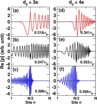
Figure 1: /Xiao, Yakubo, and Yu

Figure 1 shows, for the longitudinal polarization (along the chain axis $\hat{x}$), the real part of dipole moments obtained via ${\boldsymbol{p}}={\boldsymbol{G}}^{-1}(\omega){\boldsymbol{v}}$, where ${\boldsymbol{G}}^{-1}(\omega)$ is evaluated at a real valued frequency $\omega$ indicated in every panel. Weber04 In these calculations, we have set all but the row of $N/2$ in ${\boldsymbol{v}}$ (a column vector) equal to zero. The GPW parameters are $\epsilon_{\ell}=3.0$, $c=1.0$, $N=100$, and interparticle distance $d_{0}=4a$ ($3a$) for the left (right) panels, where $a$ is the radii of the nanoparticles. To highlight the graded effect, only near-field couplings (${\tilde{T}_{nm}}\propto 1/\left|x_{n}-x_{m}\right|^{3}$) are taken into account. We note that the fully retarded couplings were shown to be remarkably important in the case of transverse polarization. Weber04 ; Citrin06 However, their role in modifying the dispersion is a subject of controversy. Polman06 These issues become more ambiguous in the presence of loss (radiative or nonradiative), which needs to be addressed appropriately further. Here we mainly focus on the longitudinal polarization.note0 The demonstrated localizations shall hold even with full couplings included,Weber04 ; Citrin06 ; Polman06 in view of a recent exploration in the localized vibrations of optically (long-range) bounded structures.Chan06 It is seen in Fig. 1 that there exist several different solutions which correspond to modes excited by external periodic “forces” subject to the central site $n=N/2$ with different frequencies: (1) at relatively low frequency, modes are excited in the right-hand side (larger $\epsilon_{2}$), which implies the externally injected energy moves to the right [Figs. 1(a) and 1(d)]; (2) at intermediate frequency, it propagates to both sides [Figs. 1(b) and 1(e)]; (3) while at high frequency, it tends going to the left [Figs. 1(c) and 1(f)]. We can regard these excitation modes as being localized or extended depending on their spatial extent. However, if $\Gamma$ is large, we can not simply regard the solutions (not shown) in this way. This is because it is hard to distinguish the localization effect from the loss which leads to attenuation of the excitation in the medium. Busch05

In order to gain more insights into the peculiar and principal characteristics of GPWs, we therefore focus on weak loss or lossless regime hereafter. It is possible to linearize Eq. (1) with respect to $\omega^{2}$

$$({\boldsymbol{F}}-\omega^{2}{\boldsymbol{I}}){\boldsymbol{p}}=0,$$ (2)

where $\boldsymbol{I}$ is identity matrix and $F_{nm}=\omega_{n}^{2}-{G_{nm}}(\omega_{n}^{2})/G^{\prime}_{nn}(\omega_{n}^{2})$. Swith06 Here the prime indicates derivative with respect to $\omega^{2}$ and $\omega_{n}$ is the dipolar Mie resonant frequency of the $n$-th particle. Equation (2) represents a good approximation of Eq. (1) at $\omega\approx\omega_{n}$. In considering the case of weak loss, we can write the eigenspectrum {$\omega_{\alpha}=\omega^{\prime}_{\alpha}+i\omega^{\prime\prime}_{\alpha},{{\boldsymbol{p}}_{\alpha}}\}$ and ${\boldsymbol{v}}=\sum_{\alpha}\mu_{\alpha}{{\boldsymbol{p}}_{\alpha}}$. If the frequency $\omega$ is close to a eigenfrequency $\omega_{\alpha_{0}}$ then significant contribution to ${\boldsymbol{p}}$ comes from a few eigenmodes whose eigenfrequency is close to $\omega$. Let us call the set of modes $S$ that has significant contribution: $|\omega^{\prime}_{\alpha}-\omega^{\prime}_{\alpha_{0}}|\ll\omega^{\prime\prime}_{\alpha}~{}~{}\text{for}~{}~{}{\alpha}\in S.$ Thus, the real part of the response function (e.g., plotted in Fig. 1) is $\text{Re}[{\boldsymbol{p}}]=\sum_{\alpha\in S}\mu_{\alpha}(\omega-\omega^{\prime}_{\alpha}){{\boldsymbol{p}}}_{\alpha}/2\omega[(\omega-\omega^{\prime}_{\alpha})^{2}+{\omega^{\prime\prime}_{\alpha}}^{2}]$. This means by solving ${\boldsymbol{p}}={\boldsymbol{G}}^{-1}(\omega){\boldsymbol{v}}$ for weak loss in the Drude model, the solutions we get in Figs. 1(a)–1(f) are very close to a single complex eigenmodes in the GPWs.

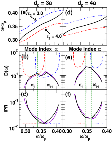
Figure 2: /Xiao, Yakubo, and Yu

In the linearized lossless case, the coupled plasmon dispersion can be directly obtained by diagonalizing ${\boldsymbol{F}}$, resulting in real eigenspectrum {$\omega_{\alpha},{\boldsymbol{p}}_{\alpha}\}$. Swith06 The results are shown in Figs. 2(a) and 2(d) (solid lines). Still these are in the near-field coupling approximation, for the same GPW structures studied in Fig. 1 except for $\Gamma=0$ now. Also the density of states (DOS) $D(\omega)=\sum_{\alpha}\delta(\omega-\omega_{\alpha})/N$ are shown in Figs. 2(b) and 2(e). The real valued eigenmodes ${\boldsymbol{p}}_{\alpha}$ (not shown) have quite different spatial extents, much like the excitation patterns in Fig. 1. This is also reflected by their inverse participation ratioSwith06 (IPR) $\sum_{n=1}^{N}{\boldsymbol{p}}_{\alpha}^{4}(n)/\left[\sum_{n=1}^{N}{\boldsymbol{p}}_{\alpha}^{2}(n)\right]^{2}$ shown in Figs. 2(c) and 2(f). The IPR is of the order of $1/N$ if modes are extended over the system with $N$ degrees of freedom, while it becomes larger than $1/N$ for spatially localized modes. We see that relatively low frequency modes are localized at the side of larger $\epsilon_{2}$ while high frequency modes are localized at the side of smaller $\epsilon_{2}$. We name these modes as “heavy gradons” and “light gradons”, respectively. More interestingly, coupled plasmon modes at intermediate frequencies between two transition points $\omega_{\text{L}}(d_{0},c)<\omega<\omega_{\text{H}}(d_{0},c)$ are extended Swith06 when $d_{0}=3a$ [corresponding to Fig. 1(b)], but are still somehow localized, rather at the central part of the GPW for $d_{0}=4a$ [corresponding to Fig. 1(e)]. These center-localized modes resemble light gradons [corresponding to Figs. 1(c) and 1(f)] at the left tail while look like heavy gradons [corresponding to Figs. 1(a) and 1(d)] in the right front, therefore are called “light-heavy gradons.”

Equation (2) can be mapped into an equivalent chain of graded coupled harmonic oscillators with additional on-site potentials. gradon In this case, the vibrating mass $M_{n}=[1+2\epsilon_{2}(x_{n})]^{2}/3\lambda\omega_{p}^{2}\epsilon_{2}(x_{n})$, and the strength of the additional harmonic spring $U_{n}=M_{n}\omega_{n}^{2}-2K_{0}$, where $K_{0}=(a/d_{0})^{3}$ is a force constant between adjacent masses, $\lambda=2$ ($-1$) for longitudinal (transverse) case. Swith06 We then define two characteristic frequencies $\omega_{c1}(n)=\sqrt{U_{n}/M_{n}}$ and $\omega_{c2}(n)=\sqrt{(U_{n}+4K_{0})/M_{n}}$. It is easy to notice that $\omega_{c1}(n)\to\omega_{n}$ and $\omega_{c2}(n)\to\omega_{n}$ when $d_{0}\to\infty$, which are as expected because the coupling between the particles vanishes for infinitely large separation. We previously shown that when $\omega_{c1}(1)<\omega_{c2}(N)$, one get extended modes between $\omega_{\text{L}}(d_{0},c)<\omega<\omega_{\text{H}}(d_{0},c)$, where $\omega_{\text{L}}(d_{0},c)=\omega_{c1}(1)$ and $\omega_{\text{H}}(d_{0},c)=\omega_{c2}(N)$. Swith06 However, if $\omega_{c1}(1)>\omega_{c2}(N)$, there is no extended modes but light-heavy gradons when $\omega_{\text{L}}(d_{0},c)<\omega<\omega_{\text{H}}(d_{0},c)$, where $\omega_{\text{L}}(d_{0},c)=\omega_{c2}(N)$ and $\omega_{\text{H}}(d_{0},c)=\omega_{c1}(1)$. Furthermore, there exists a critical point of $d_{0}=d_{c}$ when $\omega_{c1}(1)=\omega_{c2}(N)$, showing only one light-heavy gradon which, however, is across the whole system like an extended mode. These arguments work well in view of the fact that both the band boundaries and the transition frequencies [$\omega_{\text{L}}(d_{0},c)$ and $\omega_{\text{H}}(d_{0},c)$] agree with the numerical data: the two transition frequencies are marked by the vertical dashed lines in Figs. 2(b)–2(f) where they meet with the singularities in the DOS curve (thick dark lines).

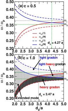
Figure 3: /Xiao, Yakubo, and Yu

As there are various plasmon modes sustained by GPWs, we construct a phase diagram as Fig. 3, which shows not only the case of $c=1.0$ [Fig. 3(b)] but also the case of $c=0.5$ [Fig. 3(a)]. Nevertheless, let us focus on Fig. 3(b) for the discussion. Figure 3(b) contains four curves of $\omega_{c1}(1)$, $\omega_{c1}(N)$, $\omega_{c1}(1)$, and $\omega_{c2}(N)$ as functions of $d_{0}$. As we have mentioned, there indeed exists a point $d_{0}=d_{c}$ (vertical dashed line) when $\omega_{c1}(1)$ and $\omega_{c2}(N)$ cross. Also we notice that $\omega_{c1}(1)=\omega_{c2}(1)\to\omega_{1}$ and $\omega_{c1}(N)=\omega_{c2}(N)\to\omega_{N}$ as $d_{0}\to\infty$, which are clearly marked by the two horizontal dashed lines of $\omega_{1}=0.378\omega_{p}$ and $\omega_{\text{N}}=0.333\omega_{p}$, respectively. In consistent with the previous results, we now discuss the four shaded regions partitioned by the four curves in Fig. 3(b). Specifically, (1) extended mode is possible only when $\omega_{c1}(1)<\omega<\omega_{c2}(N)$, and when $d_{0}<d_{c}=3.47a$ which corresponds to the left panels in Figs. 1 and 2; (2) light-heavy gradons emerge when $\omega_{c2}(N)<\omega<\omega_{c1}(1)$ for $d_{0}>d_{c}$, corresponding to the right panels in Figs. 1 and 2; (3) the lower black region indicates a phase of heavy gradons which have relatively low frequencies; (4) the upper dotted region indicates a phase of light gradons which have relatively high frequencies. Similarly, the same phase regions exist in Fig. 3(a), where a reduced $c=0.5$ results in an increased $d_{c}=4.27a$, but the discussions on the four phases through (1)$-$(4) are still applicable. In fact, the critical $d_{c}$ is determined by $\omega_{c1}(1)=\omega_{\text{L}}(d_{0},c)=\omega_{\text{H}}(d_{0},c)=\omega_{c2}(N)$ which yields

$$\frac{1}{1+2\epsilon_{2}(x_{1})} - \frac{1}{1+2\epsilon_{2}(x_{\text{N}})}=6\lambda K_{0}$$ (3)

$$\times \left(\frac{\epsilon_{2}(x_{1})}{[1+2\epsilon_{2}(x_{1})]^{2}}+\frac{\epsilon_{2}(x_{\text{N}})}{[1+2\epsilon_{2}(x_{\text{N}})]^{2}}\right).$$

The results from Eq. (3) are shown in Fig. 4(d) for both $\epsilon_{\ell}=3.0$ and $\epsilon_{\ell}=1.0$. This is a guideline for determination of extended modes. note For instance, only the region below the solid line (shaded region) supports extended modes, for the case of $\epsilon_{\ell}=3.0$. Note that in this region there exist also light and heavy gradons, depending on the frequency, whereas the region above the solid line indicates appearance of localized modes only, orderly in the form of heavy gradon, light-heavy gradon, and light gradon as frequency increases.

Up to now, we have already interpreted the mode transitions in view of the equivalent coupled harmonic oscillators of graded masses and on-site potentials. From another perspective, we further examine the relationship between the site Mie resonance of isolated nanoparticle, the resonant band of an infinite PW, and the resonant band of an infinite GPW with infinitesimal gradient. In Fig. 2 we have already plotted the corresponding results for the chains in homogeneous host of $\epsilon_{2}=\epsilon_{\ell}$ (dash-dotted lines) and $\epsilon_{2}=\epsilon_{\ell}+c$ (dashed lines), i.e., results for homogeneous PWs. It is known that infinite periodic PWs have resonant bands around respective Mie resonance $\omega_{n}$ as Weber04 ; Brongersma00

$$\omega^{2}=\omega_{n}^{2}-2\lambda\gamma_{n}^{2}\cos(kd_{0})\cosh(\tau d_{0}),$$ (4)

where $k$ is the wave number of the plasmon wave, $\tau$ the attenuation coefficient. Here the nearest-neighboring electrodynamic coupling strength $\gamma_{n}^{2}=\gamma_{0n}^{2}K_{0}$, where $\gamma_{0n}$ is host-dependent. Brongersma00 The second-order correction due to dissipations is typically $\cosh(\tau d_{0})\sim 1.001$ for silver, Brongersma00 which is negligible. Let us break the GPW into a large number of infinite segments of PWs, each of which approximated by homogeneous host $\epsilon_{2}(x_{n})$. For each of these segments we have Eq. (4), which means a series of bands located at different Mie resonance $\omega_{n}$. Overlapping of these bands can be used as guideline to determine mode types, as sketched in Fig. 4(a). In Fig. 4(b), increased $d_{0}$ defies the overlapping of these bands, therefore extended modes can not show up. For fixed $d_{0}=4a$, decreasing the gradient coefficient to $c=0.5$ will overlap all these bands again, resulting in extended modes [see Fig. 4(c)]. In this way, the critical interparticle distance $d_{c}$ is determined by the condition that the lower band edge of Eq. (4) for $\epsilon_{2}=\epsilon_{2}(x_{1})$ equals to the upper band edge for $\epsilon_{2}=\epsilon_{2}(x_{\text{N}})$, i.e., $\omega_{1}^{2}-2\lambda\gamma_{1}^{2}=\omega_{\text{N}}^{2}+2\lambda\gamma_{\text{N}}^{2}$ which simplifies to

$$\frac{1}{1+2\epsilon_{2}(x_{1})}-\frac{1}{1+2\epsilon_{2}(x_{\text{N}})}=\lambda K_{0}\left(\frac{\gamma_{01}^{2}}{\omega_{p}^{2}}+\frac{\gamma_{0\text{N}}^{2}}{\omega_{p}^{2}}\right),$$ (5)

where $\gamma_{0n}$ more explicitly depends on the resonant frequency $\omega_{n}$, the optical effective electron mass $m_{n}^{*}$, and the magnitude of the oscillating charge $Q$. For example, one can write $\gamma_{0n}^{2}=Qe/m_{n}^{*}\epsilon_{2}(x_{n})$, Brongersma00 where $e$ is the electron charge. Note that $\omega_{p}^{2}=Qe/m_{0}^{*}$, Jackson1975 we therefore get

$$\gamma_{0n}^{2}=\frac{3\omega_{n}^{2}\epsilon_{2}(x_{n})}{1+2\epsilon_{2}(x_{n})}\equiv\frac{1}{M_{n}\lambda}$$ (6)

and

$$m^{*}_{n}=m^{*}_{0}\frac{[1+2\epsilon_{2}(x_{n})]^{2}}{3\epsilon^{2}_{2}(x_{n})}.$$ (7)

Here $m^{*}_{0}$ denotes the optical effective electron mass of bulk metal in vacuum. While a free electron mass $m_{0}=9.1095\times 10^{-28}$ g, typically $m^{*}_{0}=8.7\times 10^{-28}$ g for Ag. Johnson ; Brongersma00 Equation (7) does not account for size and quantum effects in the nanoparticle, however, it is a scale relation which indicates that the optical effective electron mass increases from left to the right in the GPWs. This is consistent with our terminologies of light, heavy, and light-heavy gradons. Also it is easy to show that Eq. (5) is exactly the same as Eq. (3).

In conclusion, we have proposed GPW structures which sustain interestingly localized coupled plasmon modes that may have potential applications in plasmonics, such as optical switcher and multiplexer. The underlying localization mechanism and our analysis equally apply to a wide spectrum of analogous problems, which may have important ramifications for understanding excitations with transitional spectra in many condensed matter systems.

This work was supported in part by the RGC Earmarked Grant of the Hong Kong SAR Government (K.W.Y.), and in part by a Grant-in-Aid for Scientific Research from Japan Society for the Promotion of Science (No. 16360044).

Figure Captions

FIG. 1. (Color online) Real part of the induced dipole moment for longitudinal excitation at $i=N/2$ in a GPW for $d_{0}=3a$ (left panels) and $d_{0}=4a$ (right panels). Damping parameter $\Gamma=0.001\omega_{p}$ through (a) - (f). Real frequencies are indicated in each panel.

FIG. 2. (Color online) Dispersion relation, density of states $D(\omega)$, and inverse participation ratio (IPR) of GPW for $d_{0}=3a$ (left panels) and $d_{0}=4a$ (right panels). Dashed-dotted and dashed lines represent the corresponding results for PW in homogeneous host of $\epsilon_{2}=3.0$ and $\epsilon_{2}=4.0$, respectively. (a), (d) Dispersion relations for near field coupling. (b), (e) $D(\omega)$ versus coupled plasmon mode frequency. The thick black lines represent results of GPW with nearest-neighboring coupling. (c), (f) IPR versus frequency.

FIG. 3. (Color online) Phase diagram showing the variation of the four characteristic frequencies as functions of $d_{0}$ for (a) $c=0.5$ and (b) $c=1.0$, in the case of $\epsilon_{\ell}=3.0$. The critical interparticle distance $d_{c}$ is represented by the vertical dashed lines, whereas the two horizontal lines represent $\omega_{1}$ and $\omega_{\text{N}}$, respectively.

FIG. 4. (Color online) (a)–(c) Schematics of “band construction” in GPWs. (d) Critical interparticle distance $d_{c}$ as a function of $c$ for both $\epsilon_{\ell}=3.0$ (solid line) and $\epsilon_{\ell}=1.0$ (dashed line). The horizontal dashed line represents $d_{0}=2a$, which is the geometric limit. Extended modes are possible only in the region below these curves, e.g., shaded region in the case of $\epsilon_{\ell}=3.0$.

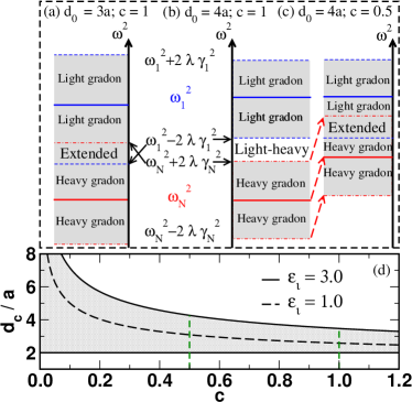
Figure 4: /Xiao, Yakubo, and Yu

References

- (1) W. L. Barnes, A. Dereux, and T. W. Ebbesen, Nature (London) 424, 824 (2003); A. V. Zayats, I. I. Smolyaninov, and A. A. Maradudin, Phys. Rep. 408, 131 (2005); E. Hutter and J. H. Fendler, Adv. Mater. 16, 1685 (2004); C. Girard, Rep. Prog. Phys. 68, 1883 (2005).
- (2) S. A. Maier and H. A. Atwater, J. Appl. Phys. 98, 011101 (2005).
- (3) M. Quinten, A. Leitner, J. R. Krenn, and F. R. Aussenegg, Opt. Lett. 23, 1331 (1998); S. A. Maier, P. G. Kik, H. A. Atwater, S. Meltzer, E. Harel, B. E. Koel, and A. A. G. Requicha, Nature Mater. 2, 229 (2003).
- (4) M. L. Brongersma, J. W. Hartman, and H. A. Atwater, Phys. Rev. B62, R16356 (2000).
- (5) W. H. Weber and G. W. Ford, Phys. Rev. B70, 125429 (2004).
- (6) D. S. Citrin, Nano Lett. 4, 1561 (2004); Nano Lett. 5, 985 (2005); Opt. Lett. 31, 98 (2006).
- (7) U. Hohenester and J. Krenn, Phys. Rev. B72, 195429 (2005).
- (8) J. J. Xiao, K. Yakubo, and K. W. Yu, Phys. Rev. B73, 054201 (2006); 73, 224201 (2006).
- (9) J. J. Xiao, K. Yakubo, and K. W. Yu, Appl. Phys. Lett. 88, 241111 (2006).
- (10) A. F. Koenderink and A. Polman, Phys. Rev. B74, 033402 (2006).
- (11) In the near-field approximation, the results of transverse polarizations (not shown here) are similar, except for a narrower band due to smaller coupling strength as compared to the case of longitudinal polarization. However, with fully retarded coupling, polariton-like anticrossing in the dispersion is expected for transverse polarizations (see Ref. 10). This should be true in GPWs even though phase matching is apparently not observed.
- (12) J. Ng and Chan C. T. Chan, Opt. Lett. 31, 2583 (2006); J. Ng, C. T. Chan, P. Sheng P, and Z. F. Lin, Opt. Lett. 30, 1956 (2006).
- (13) A. Lubatsch, J. Kroha, and K. Busch, Phys. Rev. B71, 184201 (2005).
- (14) P. B. Johnson and R. W. Christy, Phys. Rev. B6, 4370 (1972).
- (15) From this argument, it is evident that the extended modes at intermediate frequencies are not a consequence of the end effects that constrain the high- and low-frequency response, but rather due to the effective on-site potential () confinment, quite similar to Ref. 12. Therefore, these extended modes persist even for infinite-size systems in the infinitesimal gradient limit.
- (16) J. D. Jackson, Classical Electrodynamics (Wiley, New York, 1975).