Pressure Driven Flow of Polymer Solutions in Nanoscale Slit Pores

Abstract

Polymer solutions subject to pressure driven flow and in nanoscale slit pores are systematically investigated using the dissipative particle dynamics approach. We investigated the effect of molecular weight, polymer concentration and flow rate on the profiles across the channel of the fluid and polymer velocities, polymers density, and the three components of the polymers radius of gyration. We found that the mean streaming fluid velocity decreases as the polymer molecular weight or/and polymer concentration is increased, and that the deviation of the velocity profile from the parabolic profile is accentuated with increase in polymer molecular weight or concentration. We also found that the distribution of polymers conformation is highly anisotropic and non-uniform across the channel. The polymer density profile is also found to be non-uniform, exhibiting a local minimum in the center-plane followed by two symmetric peaks. We found a migration of the polymer chains either from or towards the walls. For relatively long chains, as compared to the thickness of the slit, a migration towards the walls is observed. However, for relatively short chains, a migration away from the walls is observed.

I INTRODUCTION

The transport of polymer solutions in small confining geometries remains a long stranding topic with many unanswered questions. The understanding of the transport of polymer solutions is important to chromatography, electrophoresis, adhesion, lubrication, polymer processing, oil recovery, etc. Recently, there has been an increasing interest in the areas of macromolecular transport in channels with widths comparable to size of a single molecule agarwal94 . For example, the understanding of the structure and dynamics of polymeric molecules in micro-channels is important to DNA sequencing in channels with widths ranging from $10$ to $50\mu{\rm m}$ fang05 , DNA delivery through micro-capillaries in gene therapy, and to lab-on-chip applications that involve polymers han00 . Issues of particular interest pertinent to polymer solutions in the presence of laminar flow is the mass distribution of polymers across the channel, the polymers conformational distribution, and the effect of the polymer chains on the profile of the solution velocity field  muller90 ; ausserre91 ; agarwal94 ; horn00 ; shrewsberry01 ; fan03 ; fang05 ; woo04_1 ; woo04_2 ; jendrejack04 ; ma05 ; usta05 ; usta06 ; khare06 .

Past experiments were performed to investigate the conformational changes of polymers in the presence of elongational flow by Perkins et al. perkins97 and in the presence of shear flow by Smith et al.  smith99 through tracking fluorescently labeled DNA molecules. These experiments showed that the polymer chains become elongated along the flow direction. Several experiments indicated the existence of a depletion layer in the polymers near the confining walls muller90 ; ausserre91 ; agarwal94 ; horn00 ; shrewsberry01 . The recent experiment by Horn et al. horn00 on a dilute solution of a high molecular weight polyisobutene in a very viscous fluid observed that the polymer solution exhibits flow with an apparent slip at the boundary.

It is well known that at equilibrium conditions, polymer chains near walls, and in the non-adsorbed regime, are sterically depleted from the wall due their reduced conformational entropy degennes79 . In the presence of a pressure-driven (Poiseuille) flow, the shear rate across the channel is non-uniform. As a result, one expects a higher concentration of polymers in the mid-section of the channel since, there, the local shear is lowest, leading thereby to an apparent slip at the walls fang05 . Due to the additional stretching of the polymer chains near the walls, as a result of the shear stresses originating from finite shear rate, thermodynamic arguments predict that the thickness of the depletion layer is thinner when compared to that at equilibrium conditions. Consequently, the steric effect of the walls on the polymer chains is less severe than at equilibrium conditions. However, experiments agarwal94 on dilute polymer solutions demonstrated that even in the case of uniform shear flow, the polymer chains migrate away from the wall leading to a depletion layer that is wider than at equilibrium. Therefore, the thermodynamic arguments alone are unable to fully account for the migration of the polymer chains observed in experiments. It is important to note that since these systems are not at equilibrium, thermodynamic arguments are not applicable.

The understanding of the migration of the polymer chains away from the wall must therefore take into account hydrodynamic interactions in the solution. However, such understanding is complicated by the non-Newtonian properties of polymer solutions. Theories have therefore been based on simplified systems rather than on polymer solutions. Previous theoretical and computational studies that focused on the density profiles of polymers in uniform shear flow (i.e., Couette flow) or pressure driven flow (i.e., Poiseuille flow) have been conflicting woo04_1 ; woo04_2 ; ma05 ; usta05 ; usta06 . Previous Brownian dynamics simulations showed a migration of the polymer chains towards the wall woo04_1 ; woo04_2 . In these studies, however, wall-monomer hydrodynamic interactions are not accounted for. A recent kinetic theory by Ma and Graham ma05 of an infinitesimally dilute solution of dumbbells predicts a migration of the dumbbell particles away from the wall towards the mid-section of the channel. A key reason for the migration of the dumbbells away from the wall is attributed to the hydrodynamic interaction between the wall and the dumbbell, which leads to a deterministic migration from the wall, while the effect of the Brownian motion is to homogenize the solution and therefore to counter the effect of the wall-monomer hydrodynamic interaction. This cross-stream migration was recently investigated numerically by Jendrejack et al. using a Brownian dynamics simulation that self-consistently accounts for both monomer-monomer hydrodynamic interaction and wall-monomer hydrodynamic interaction jendrejack04 . In this study, they observed that in the presence of pressure driven flow, the polymer density profile exhibits a local minimum (a dip) in the middle of the pore, which decreases as the flow rate is increased. They also observed that the depletion region from the walls is amplified as the flow rate is increased. The depletion from the wall becomes substantial for large flow rates. In the more recent simulations by Usta et al. usta05 ; usta06 , which are based on a bead model for the polymer chains coupled to a lattice Boltzmann description for the solvent, the polymer density profile was also found to exhibit a minimum in the center-plane of the slit followed by two symmetric maxima. Near the wall, a migration away from the wall is observed when the ratio between the thickness of the slit and the equilibrium radius of gyration of the polymer chains is large, i.e., in the weak confinement regime. However, when confinement is increased, a migration towards the wall is observed. This result contrasts that of Jendrejack et al. jendrejack04 , where even in the strong confinement regime, a migration away from the wall is observed. In the presence of uniform shear flow, Usta et al. usta06 observed that the density profile does not exhibit a peak in the mid-section of the slit, instead of a dip. The presence of a dip in the mid-section of the slit must therefore be associated with gradients in the shear rate, present in pressure driven flow.

Very recently, Khare et al. used molecular dynamics to study the density profile of dilute polymer solutions in both uniform shear flow and pressure driven flow khare06 . In the case of pressure driven flow, they also observed a local minimum in the polymer density profile. However, the depletion layer is only weakly modified by flow. As in Usta et al.’s work usta06 , Kare et al. also observed that the polymer density profile peaks in the mid section of the slit in the case of uniform shear flow. A recent simulation by Fan et al. fan03 based on dissipative particle dynamics of dilute polymer solutions in pressure driven flow in a slit channel focused on the velocity profile of the polymer solutions. In their study however, they studied the migration of dimers instead of chains, and they observed very weak migration fan03 . Therefore, the issue of migration clearly remains settled, warranting further investigation.

A large number of studies during recent years have proved that dissipative particle dynamics (DPD) is a successful explicit computational approach in the investigation of both equilibrium and non-equilibrium properties of complex fluids. A recent study by Ripoll et al. showed, in particular, that DPD correctly describe large scale and mesoscopic hydrodynamics in fluids ripoll01 . Using extensive DPD simulations, we recently investigated equilibrium dynamics of polymer chains in the dilute and concentrated regimes, and both in bulk and in confining geometries. We found that the chains dynamics is well described by the Zimm model in the dilute regime, and as expected a crossover to Rouse dynamics is observed as the polymer concentration is increased jiang06 ; jiang07 . These studies validate the usefulness of DPD in correctly describing the dynamics of polymer solutions. We therefore used the DPD approach in studying the dynamics of polymer solutions in pressure driven flow.

In the present article, we present results based on DPD simulations of polymer solutions in nanoscale slits and in the presence of pressure driven flow. Our study is performed on systems with various polymer volume fractions, chain length, and flow rate. We will particularly discuss the velocity profile of the solution across the channel, the conformational distribution of the polymer chains and their mass distribution. In Sec. 3, we present results of Poiseuille flow of a simple fluid using DPD. In Sec. 4, the model and computational approach is presented. In Sec. 3, we present and discuss the numerical results. Finally, we summarize and conclude in Sec. 5.

II MODEL AND METHOD

In this work, we investigate the dynamics of dilute and semi-dilute polymer solutions under pressure driven flow using the dissipative particle dynamics (DPD) approach. DPD was first introduced by Hoogerbrugge and Koelman more than a decade ago hoogerbrugge92 , and was cast in its present form about five years later espagnol95 ; espagnol97 . DPD is reminiscent of molecular dynamics, but is more appropriate for the investigation of generic properties of macromolecular systems. The use of soft repulsive interactions in DPD, allows for larger integration time increments than in a typical molecular dynamics simulation using Lennard-Jones interactions. Thus time and length scales much larger than those in atomistic molecular dynamics simulations can be probed by the DPD approach. Furthermore, DPD uses pairwise random and dissipative forces between neighboring particles, which are interrelated through the fluctuation-dissipation theorem. The pairwise nature of these forces ensures the local conservation of momentum, a necessary condition for correct long-range hydrodynamics pagonabarraga98 ; ripoll01 . The DPD approach was recently used for the study of flow of colloidal suspensions palma06 and flow of dilute polymer solutions fan03 ; fan06 .

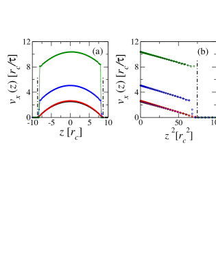
Figure 1: (a) Velocity field along the $x$-axis vs. $z$ for the case of a driving force, $f_{x}=0.02\epsilon/r_{c}$. Curves from bottom to top correspond to wall-solvent interaction parameter $a_{ws}=3\epsilon/r_{c}$, $10\epsilon/r_{c}$, $20\epsilon/r_{c}$, and $30\epsilon/r_{c}$, respectively. (b) The velocity profile vs. $z^{2}$. Not that $v_{x}(z)$ is quadratic in $z$ regardless of the wall-solvent interaction. The vertical dot-dashed lines indicate the positions of the walls. Notice that curves for $a_{ws}=3\epsilon/r_{c}$ and $10\epsilon/r_{c}$ overlap with each other.

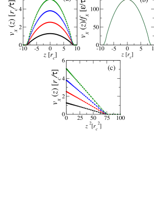
Figure 2: (a) Velocity field along the $x$-axis vs. $z$ for $a_{ws}=3\epsilon/r_{c}$. Curves from bottom to top correspond to a driving force $f_{x}=0.01$, 0.02, 0.03, and $0.04\epsilon/r_{c}$. (b) The velocity profile normalized by the driving force vs. $z$. The excellent collapse in (b) implies that the velocity profile follows Eq. (13). (c) The velocity profile vs. $z^{2}$.

In the DPD approach, two particles, $i$ and $j$, interact with each other via three pairwise forces corresponding to a conservative force, ${\bf F}^{(C)}_{ij}$, a dissipative force, ${\bf F}^{(D)}_{ij}$, and a random force, ${\bf F}^{(R)}_{ij}$. These three forces are respectively given by,

$${\bf F}^{(C)}_{ij} = a_{ij}\omega(r_{ij}){\bf n}_{ij},$$ (1)

$${\bf F}^{(D)}_{ij} = \gamma_{ij}\omega^{2}(r_{ij})(\hat{\bf r}_{ij}\cdot{\bf v}_{ij}){\bf n}_{ij},$$ (2)

$${\bf F}^{(R)}_{ij} = \sigma_{ij}(\Delta t)^{1/2}\omega(r_{ij})\theta_{ij}{\bf n}_{ij},$$ (3)

where ${\bf r}_{ij}={\bf r}_{j}-{\bf r}_{i}$, ${{\bf n}}_{ij}={{\bf r}_{ij}}/{r_{ij}}$, and ${\bf v}_{ij}={\bf v}_{j}-{\bf v}_{i}$. $\theta_{ij}$ is a symmetric random variable satisfying

$$\langle\theta_{ij}(t)\rangle = 0,$$ (4)

$$\langle\theta_{ij}(t)\theta_{kl}(t^{\prime})\rangle = (\delta_{ik}\delta_{jl}+\delta_{il}\delta_{jk})\delta(t-t^{\prime}).$$ (5)

with $i\neq j$ and $k\neq l$. In Eq.(3), $\Delta t$ is the iteration time step. The weight factor is chosen as

$$\omega(r)=\left\{\begin{array}[]{ll}1-r/r_{c}&\mbox{ for $r\leq r_{c}$,}\\ 0&\mbox{ for $r>r_{c}$}\end{array}\right.$$ (6)

where $r_{c}$ is the interactions cutoff radius. The choice of $\omega$ in Eq. (6) ensures that the interactions are all soft and repulsive. The values of the parameter $a_{ij}$ used in the simulations are specifically chosen as

$$a_{ij}=\frac{\epsilon}{r_{c}}\left(\begin{array}[]{cccc}&w&s&p\\ w&-&3&10\\ s&3&25&25\\ p&10&25&50\\ \end{array}\right),$$ (7)

where $w$, $s$ and $p$ designate a wall, solvent and a monomer particle, respectively. We should not that $a_{ww}$ is irrelevant since the wall particles are kept frozen in the simulation. The importance of the wall-solvent interaction to the velocity field boundary condition will be discussed in Section III. The integrity of a polymer chain is ensured via an additional harmonic interaction between consecutive monomers,

$${\bf F}_{i,i+1}^{(S)}=-C\left(1-r_{i,i+1}/b\right){{\bf n}}_{i,i+1},$$ (8)

where we set, for the spring constant and the preferred bond length, $C=100\epsilon$ and $b=0.45r_{c}$, respectively.

The equations of motion of particle $i$ are given by

$$d{\bf r}_{i}(t) = {\bf v}_{i}(t)dt,$$ (9)

$$d{\bf v}_{i}(t) = \frac{1}{m}\sum_{j}[{\bf F}^{(C)}_{ij}dt+{\bf F}^{(D)}_{ij}dt$$ (10)

$$+ {\bf F}_{ij}^{(R)}(dt)^{1/2}],$$

where $m$ is the mass of a single DPD particle. Here, for simplicity, masses of all types of dpd particles are supposed to be equal. Assuming that the system is in a heat bath at a temperature $T$, the parameters $\gamma_{ij}$ and $\sigma_{ij}$ in Eqs. (2) and (3) are related to each other by the fluctuation-dissipation theorem,

$$\gamma_{ij}=\sigma_{ij}^{2}/2k_{\rm B}T.$$ (11)

Consider a fluid in a pore of cross section ${\cal A}$ under a pressure gradient ${\partial P}/{\partial x}$. As a result, a portion of fluid of length $dx$ along the $x$-axis experiences a net force along the direction of diminishing $P$ given by, $d{\bf F}={\cal A}dP\hat{\bf x}$. Consequently, each particle $i$ in the volume ${\cal A}dx$ experiences an additional force

$${\bf f}_{i}=f_{x}\hat{\bf x}=-\frac{1}{\rho}\biggl{|}\frac{\partial P}{\partial x}\biggl{|}\hat{\bf x},$$ (12)

to be added to the forces in Eqs. (1-3). The values of the driving force considered in the present study range from 0 to $0.04\epsilon/r_{c}$.

Most of our simulations are performed on boxes of dimensions $L_{x}\times L_{y}\times L_{z}$ with $L_{x}=L_{y}=19.6r_{c}$ and $L_{z}=20r_{c}$. We made sure that finite size effects are absent by performing simulations on boxes with larger values of $L_{x}$ and $L_{y}$. As will be discussed in the next section, a frozen wall is used. The wall is parallel to the $xy$-plane, and the flow is along the $x$-axis.

We used periodic boundary conditions in the three directions. Therefore only one wall is used. We consider a fluid with a number density $\rho=4r_{c}^{-3}$, $k_{B}T=\epsilon$, and $\sigma=3.0(\epsilon^{3}m/r_{c}^{2})^{1/4}$. We used a wall with thickness $2.8r_{c}$. The wall is constructed from dpd particles that are arranged in a face centered cubic lattice with number density $61.35r_{c}^{-3}$, and therefore much higher than that of the solvent. This is done in order to prevent the solvent particles from penetrating the wall. The iteration time $\delta t=0.01\tau$, where the time scale $\tau=(mr_{c}^{2}/\epsilon)^{1/2}$. All our simulations were at least run over a time period of $8000\tau$, corresponding to $8\times 10^{5}$ time steps. The first $1000\tau$ is used for relaxation of the system towards its steady state, and the remaining time is used for collection of the data.

III POISEUILLE FLOW OF A SIMPLE FLUID AND PARAMETER SELECTION FOR WALL-SOLVENT INTERACTION

Before presenting results on the flow of polymer solutions, it is useful to investigate the flow of the solvent alone (a Newtonian fluid) in a slit, using the DPD approach, and compare with the theoretical expectations for Poiseuille flow. We recall that in a laminar flow along the $x$-axis, the $xz$-component of the stress tensor, $\Pi_{xz}$ is related to the shear rate, $(\partial v_{x}/\partial z)$, through the relation $\Pi_{xz}=-\eta_{0}(\partial v_{x}/\partial z)$, where $\eta_{0}$ is the fluid viscosity. The solution of the steady-state Navier-Stokes equation of the incompressible Newtonian fluid $\nabla P=\eta_{0}\nabla^{2}{\bf v}$, with a no-slip boundary condition at the walls, which are perpendicular to the $z$-axis, ${\bf v}\left(z=\pm H/2\right)=0$, and under a uniform pressure drop, $(dP/dx)$ along the $x$-axis, corresponds to the usual Hagen-Poiseuille parabolic profile landau

$$v_{x}(z)=-\frac{H^{2}}{8\eta_{0}}\left(\frac{dP}{dx}\right)\left[1-\left(\frac{z}{H}\right)^{2}\right].$$ (13)

Within the DPD and molecular dynamics approaches, several techniques have been proposed to provide a no-slip wall-fluid boundary conditions. Revenga et al., for example, used an effective field, instead of a wall composed of particles, in conjunction with a reflection force to reflect particles that cross the wall revenga98 . Willemsen et al. . willemsen00 proposed a method that involves a layer of particles along the wall outside the simulation box. The coordinates and velocities of these particles are determined by mirroring those of the fluid particles within the cutoff distance of the interaction potential. The momenta of the additional particles are such that the average velocity of a fluid particle, within the cutoff distance, and its auxilary particle within the wall satisfies the desired boundary condition. In a recent study, we found that the use of a thermalized wall can also help in obtaining a no-slip boundary condition huang06 . In the current study, we found that a no-slip boundary condition can practically be obtained by lowering the wall-fluid interaction.

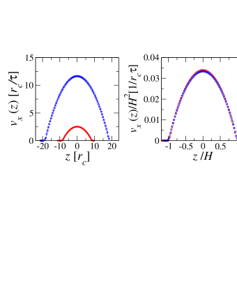
Figure 3: Velocity field along the $x$-axis vs. $z$ for $a_{ws}=3\epsilon/r_{c}$. Curves from bottom to top correspond to a driving force $f_{x}=0.01$, 0.02, 0.03, and $0.04\epsilon/r_{c}$. Inset shows the same velocity profile normalized by the driving force. The excellent collapse of all data is an implication that the velocity profile follows Eq. (13).

In Fig. 1, the velocity profile of a pure solvent is shown for the case of a slit width $L_{z}=20r_{c}$, a driving force $f_{x}=0.02\epsilon/r_{c}$ and values of the wall-solvent interaction corresponding to $a_{ws}=3\epsilon/r_{c}$, $10\epsilon/r_{c}$, $20\epsilon/r_{c}$, and $30\epsilon/r_{c}$. This figure shows that the velocity profile exhibits a discontinuity when the amplitude is large ($a_{ws}>10\epsilon/r_{c}$), implying that the fluid lubricates the wall (i.e. the wall does not act as a no-slip boundary) at large wall-solvent interactions. However for $a_{ws}\leq 10\epsilon/r_{c}$, the wall acts effectively as a no-slip boundary condition. In the remaining if this article, all simulations were performed with a wall-solvent interaction parameter $a_{ws}=3\epsilon/r_{c}$.

In Fig. 2(a), the velocity profile of the simple fluid is shown for different values of the driving force, and a wall solvent interaction, $a_{ws}=3\epsilon/r_{c}$. As shown in Fig. 2(b), the normalization of the $z$-component of the velocity field by the driving force yields a universal velocity profile, in excellent agreement with the theoretical prediction for Poiseuille flow, Eq. (13). We also tested the scaling of the velocity profile with the width of the slit pore. As shown in Fig. 3, we found again that the scaling of the velocity profile with the width of of the slit is in excellent agreement with Eq. (13).

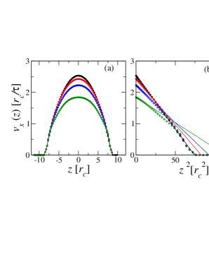
Figure 4: (a) Velocity field along the $x$-axis vs. $z$ for a polymer solution with $N=100$ and at a driving force $f_{x}=0.02\epsilon/r_{c}$. Curves from top to bottom correspond to polymer volume fraction $\varphi_{p}=0$, $0.06$, $0.12$ and $0.24$, respectively. $a_{ws}=3\epsilon/r_{c}$. (b) Same data in (a) plotted vs. $z^{2}$. The straight lines are linear fits to the data for small values of $z$.

IV POISEUILLE FLOW OF POLYMER SOLUTIONS

IV.1 Velocity Profile of Polymer Solutions in Poiseuille Flow

For a polymer solution, which is a non-Newtonian fluid, the shear stress relation to the shear rate, $(dv_{x}/dz)$, is approximated by a power law equation proposed by Ostwald wilkinson60 ,

$$\Pi_{xz}=-K\left(\frac{dv_{x}}{dz}\right)^{n},$$ (14)

where $K$ and the exponent $n$, are usually referred to as the flow consistency index and the fluid power-law index, respectively. For a polymer solution, which is a shear-thinning fluid, the power-law index $n<1$. Eq. (1) translates into a solution viscosity $\eta\sim(dv_{x}/dz)^{n-1}$. Note that Eq. (1) implies that the viscosity diverges for very low shear rates. Therefore, the power law model is not expected to hold at very low shear rates.

The balance between the driving force due to pressure gradient and the forces due to shear stresses lead to the solution,

$$v_{x}(z) = \frac{n}{1+n}K^{-1/n}\biggl{|}\frac{dP}{dx}\biggl{|}^{{1}/{n}}H^{{1}/{n}+1}$$ (15)

$$\times \left[1-\left(\frac{z}{H}\right)^{{1}/{n}+1}\right],$$

which reduces to Eq. (13) when $n=1$.

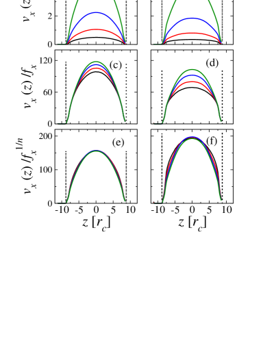
Figure 5: Fluid velocity profile across the slit for the case of (a) $\varphi=0.12$ and $N=50$ and (b) $\varphi=0.24$ and $N=100$. In (a) and (b) Curves from bottom to top correspond to $f_{x}=0.005$, $0.01$, $0.02$, and $0.04\epsilon/r_{c}$. The velocity profiles scaled by the driving force are shown for (c) $\varphi=0.12$ and $N=50$, and (d) $\varphi=0.24$ and $N=100$. The velocity profiles scaled by $f_{x}^{1/n}$ are shown in (e) $\varphi=0.12$ and $N=50$, and (f) $\varphi=0.24$ and $N=100$. In (e), $n=0.92$ and in (f), $n=0.84$. The vertical dot-dashed lines indicate the positions of the walls.

We performed a large number of systematic simulations of flow of polymer solutions for different values of chain length corresponding to $N=5$, 20, 50, and 100, polymer volume fraction corresponding to $\varphi=0.06$, 0.12, and 0.24, and driving force ranging between 0 and $0.04\epsilon/r_{c}$. In Fig. 4, the velocity profile of a polymer solution with chain length $N=100$ and under a driving force $f_{x}=0.02\epsilon/r_{c}$ is shown for volume fractions, $\varphi=0$, $0.06$, $0.12$ and $0.24$. This figure shows that except from the region close to the wall, the velocity profile is not quadratic in $z$, and therefore does not follow Hagen-Poiseuille’s law for Newtonian fluids, Eq. (13). This is due to the non-linear rheological properties of the polymer solution. In vicinity of the wall, however, the velocity profile is practically independent of $\varphi$. This is presumably due to the fact that the polymer chains are sterically depleted from the wall regions. In Fig. 4(b), an approximate linear fit of the velocity profile vs. $z^{2}$ around the mid-section of the slit leads to an effective wall boundary that extends beyond the physical boundary. This leads to the an apparent slip of the polymer solution at the wall.

In order to investigate even further the departure of the velocity profile from that Hagen-Poiseuille quadratic profile of Newtonian fluids, the velocity profiles of two polymer solutions, corresponding to $(\varphi,N)=(0.12,50)$ and $(0.24,100)$ are shown in Fig. 5. Fig. 5(c) and (d) show that, in contrast to the case of a simple fluid (see Fig. 2(b)), the velocity profile of a polymer solution does not scale linearly with the driving force, and that the departure from this scaling worsens as the chain length and/or the volume fraction of the polymers is increased. It is interesting to note that the scaling holds reasonably well close to the walls. This is due to the very low polymer density near the walls. A fit of the velocity profile with the generalized Hagen-Poiseuille equation for Non-Newtonian fluids, Eq. (15), yields power law fluid index $n=0.92$ and $n=0.84$ for the case of $(\varphi,N)=(0.12,50)$ and $(0.24,100)$, respectively. A modified scaling of the velocity profile with $f_{x}^{1/n}$ is depicted in Figs. 5(e) and 5(f) respectively. Fig. 5(e) shows that the scaling holds reasonable well in the case of relatively low volume fraction of polymer. Fig. 5(f) shows that the scaling does not hold as well in the case of $(\varphi,N)=(0.24,100)$, where both the polymer volume fraction and molecular weight are higher. This is presumably due to the fact that the exponent $n$ itself depends on the driving force, $f_{x}$.

In Fig. 6, the velocity profile for a solution with $(\varphi,N)=(0.12,50)$ under a driving force $f_{x}=0.02\epsilon/r_{c}$ is shown for two values of the slit thickness corresponding to $H=7.8r_{c}$ and $17.6r_{c}$. Fig. 6(b) shows that the scaling of the velocity profile with $H^{2}$ in the case of a polymer solution does not hold in the center-plane region, but holds reasonably well in vicinity of the walls. This is again due to the depletion of polymers from the walls region. Fig. 6(c) shows that a better scaling in the mid-section region is achieved when Eq. (15) is used with $n=0.84$.

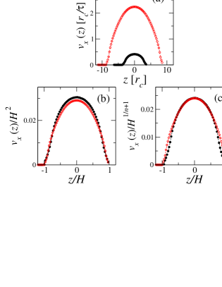
Figure 6: (a) Fluid velocity profile across the slit for the case of $\varphi=0.12$, $N=50$ and $f_{x}=0.02\epsilon/r_{c}$. Solid circles and open circles correspond to a slit thickness $H=7.8r_{c}$ and $H=17.6r_{c}$, respectively. (b) The fluid velocity scaled by $H^{2}$ vs. $z/H$. (c) The fluid velocity scaled by $H^{\frac{1}{n}+1}$ vs. $z/H$, with $n=0.84$.

We now turn our attention to the analysis of the polymers velocity profile. Since the polymers are sterically depleted from the regions near the wall, it is expected that in average the polymer chains move faster than the solvent and that the longer polymer chains move faster than the shorter polymer chains dimarzio70 . In Fig. 7, the ratio between the average polymer velocity and the average fluid velocity, $\langle v^{p}_{x}\rangle/\langle v_{x}\rangle$ is shown. This figure shows that the polymer moves faster than the solution by about $10\%$. This effect is however reduced as the polymer volume fraction is increased. This is due to the fact that across the slit, the polymers become more evenly distributed as their volume fraction is increased. Fig. 7 shows as well that as the chain length is increased, $\langle v^{p}_{x}\rangle/\langle v_{x}\rangle$ increases, mainly as a result of exclusion of the polymers from the walls. However, for $N=100$, Fig. 7 shows that $\langle v^{p}_{x}\rangle/\langle v_{x}\rangle$ is slightly smaller than that for shorter chains. Presumably, this is due to the fact that long chains tend to migrate away from the center-plane, as will be discuss later.

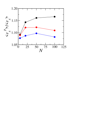
Figure 7: The ratio between average polymer velocity and solution velocity along the flow direction, $\langle v^{p}_{x}\rangle/\langle v_{x}\rangle$ as a function for chain length for $f_{x}=0.02\epsilon/r_{c}$ and $H=7.8r_{c}$. Curves from top to bottom correspond to $\phi=0.06$, $0.12$ and $0.24$, respectively.

In Fig. 8, the velocity profile of the polymer chains is shown for the case of $N=100$ at a driving force $f_{x}=0.02\epsilon/r_{c}$ for volume fractions $\varphi=0.06$, 0.12 and 0.24. This figure shows that the velocity profile of the polymer chains differs from that of the embedding solvent despite the fact that the polymer chains are transported by the solvent. Fig. 9(a) and (b) depict the velocity profiles of the fluid and the polymer for the case of $(\varphi,N)=(0.06,5)$ and $(0.06,100)$, respectively. There, it is clear that the two profiles do not coincide, particularly when the chain length or volume fraction is increased. Fig. 8 shows that the polymer velocity exhibits a sharp discontinuity near the walls of the slit, implying that as far as the polymer is concerned, the walls act as a slip boundary. Fig. 9 shows in the middle of the slit, the polymer chains move slightly slower than the embedding solvent, and that the difference between the solvent velocity and the polymer velocity is increased as the polymer chain length or volume faction is increased. Fig. 9 also shows that in the middle of the slit the polymer motion is retarded as compared to that of the solvent. However, the motion the polymers is faster than the solvent near the walls. The slower motion of the polymer chains near the walls is due to the fact that due to the monomers connectivity, monomers belonging to a single chain have to move with same average velocity.

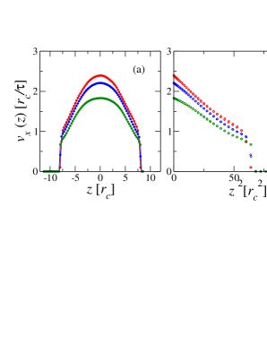
Figure 8: (a) Polymer velocity field along the $x$-axis vs. $z$ for a polymer solution with $N=100$ and at a driving force $f_{x}=0.02\epsilon/r_{c}$. Curves from top to bottom correspond to polymer volume fraction $\varphi_{p}=0.06$, $0.12$ and $0.24$, respectively. $a_{ws}=3\epsilon/r_{c}$. (b) Same data in (a) plotted vs. $z^{2}$.

IV.2 Polymers Conformational Distribution

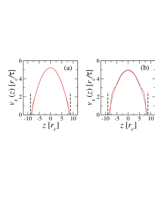
Figure 9: Solvent velocity profile (dashed line) is shown together with the polymer velocity profile (solid line) for the case of $\varphi=0.06$ and $f_{x}=0.04\epsilon/r_{c}$. (a) and (b) correspond to $N=5$ and $N=100$, respectively. The vertical dot-dashed lines indicate the positions of the walls.

We now focus on the effect of flow on the conformational distribution of the polymer chains in solution. In Fig. 10, the distributions of the three components of the radius of gyration, $R_{g}^{(x)}$, $R_{g}^{(y)}$ and $R_{g}^{(z)}$, of a polymer solution, with $N=50$ and $\varphi=0.12$ are shown for driving forces corresponding to $f_{x}=0$, $0.01\epsilon/r_{c}$, $0.02\epsilon/r_{c}$, and $0.04\epsilon/r_{c}$. The $z$-axis represents the position of the center of mass of the chains. This figure indicates that, near the walls, the $z$-component of the radius of gyration is lower than than $R_{g}^{(x)}$ and $R_{g}^{(y)}$ near the walls. This is due to the steric interactions with the walls. Fig. 10 shows that at equilibrium ($f_{x}=0$) and away from the walls, the three components of the radius of gyration are equal, implying that the chains away from the walls do not experience confinement. This implies that under non-equilibrium conditions, the redistribution of the radius of gyration is due to the flow. As the driving force is increased, the chains become stretched along the flow direction, i.e. along the $x$-axis, regardless of the location of their center of mass across the channel. This figure also shows that the chains stretching along the flow direction is lowest in the mid-section of the slit pore. This is due to the fact that the shear rate, and therefore the resulting stresses, are lowest in this region. Away from the mid-section of the slit, the chains stretching increases but in a non-monotonous fashion. In particular, we observe that the distribution of $R_{g}^{(x)}$ exhibits two peaks somewhat close, but not very close, to the wall. The positions of these two peaks along the $z$-axis approach the wall as the driving force is increased. Very close to the walls, and within the depletion layer, the stretching is again increased. A similar complex behavior of the distribution of chains radius of gyration was recently reported by Jendrejack et al. using their self-consistent Langevin dynamics approach jendrejack04 . We also note that the position of the two weak off-center maxima in the distribution of the $x$-component correlate with the onset of the shoulders in the velocity profile of the polymer chains, shown in Fig. 9(b).

Fig. 10 shows that the $y$-component of the radius of gyration, $R_{g}^{(y)}$, decreases from its maximum value at the center-plane up to some point, and then increases at distances closer to the wall. Since the shear stress $\Pi_{xy}=0$, the contraction of the chains along the $y$-axis and around the center-plane is a partial compensation to the chains stretching along the $x$-axis. The increase of the $y$-component of the radius of gyration, closer to the walls, is a compensation to the decrease of the $z$-component of the radius of gyration close to the walls. As for the $z$-component, $R_{g}^{(z)}$, its fast decrease near the walls is due to steric interactions with the walls. around the mid-plane, the decrease is slower, and is due to gradient in shear rate along the $x$-axis. As the driving force is increased, shear stresses are amplified leading to further contraction of the chains along the $z$-axis.

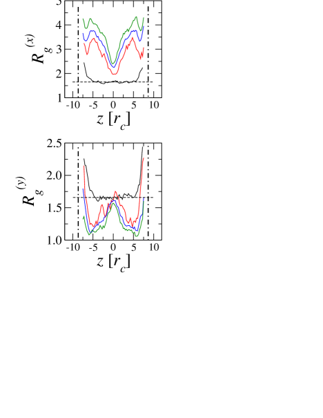
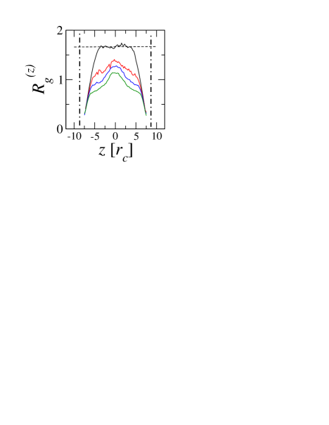
Figure 10: Distribution of the three components of chains radius of gyration along the slit for the case of $N=50$ and $\varphi=0.12$. In (x), curves from bottom to top correspond to $f_{x}=0$, $0.01\epsilon/r_{c}$, $0.02\epsilon/r_{c}$ and $0.04\epsilon/r_{c}$. In (y) and (z), curves from top to bottom correspond to $f_{x}=0$, $0.01\epsilon/r_{c}$, $0.02\epsilon/r_{c}$ and $0.04\epsilon/r_{c}$. The horizontal dashed line corresponds to the value of $R_{g}/\sqrt{3}$ of a bulk solution at equilibrium. The vertical dot-dashed lines indicate the positions of the walls.

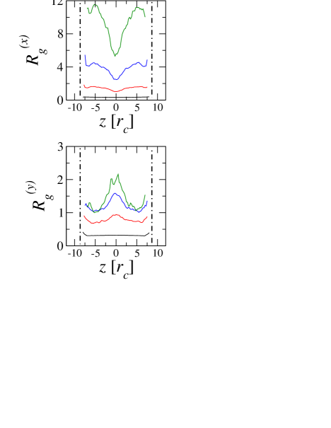
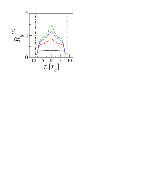
Figure 11: Distribution of the three components of chains radius of gyration along the slit for the case of $f_{x}=0.04\epsilon/r_{c}$ and $\varphi=0.12$. Curves from bottom to top correspond to $N=5$, $20$, $50$, and $100$, respectively. The vertical dot-dashed lines indicate the positions of the walls.

In Fig. 11, the profiles of the components of the radius of gyration across the channel are shown for a solution with $\varphi_{p}=0.12$ with $N=5$, 20, 50, and 100 at a driving force $f_{x}=0.04\epsilon/r_{c}$. This figure shows that the effects observed in Fig. 10 are enhanced as the chain length is increased.

IV.3 Polymers Density Profile

In Fig. 12(a), the monomers distribution in the case of a dilute solution with $\varphi=0.06$ and $N=100$ is shown for three values of the driving force corresponding to $f_{x}=0$, 0.02 and $0.04\epsilon/r_{c}$. This figure shows that at equilibrium conditions ($f_{x}=0$) and away from the walls, the distribution is, as expected, essentially uniform. However, in the presence of flow, the distribution exhibits a local minimum in the center-plane. This figure also shows that the thickness of the depletion layer slightly decreases as the driving force is increased. This figure therefore implies that for this specific $\varphi$ and $N$, the polymer chains migrate away from the center-plane towards the walls. We note that in this case the ratio between the slit thickness and the chain radius of gyration is $2H/R_{g}\approx 3.6$. For this ratio, Usta et al. also found a migration towards the wall usta06 . In the case of weak confinement, $\phi=0.06$ and $N=20$ (for which $2H/R_{g}\approx 10.8$), we also found a peak in the middle of the slit, although the peak is weaker than for $N=100$. Near the walls, we found a slight increase in the depletion layer, again in qualitative agreement with Usta et al.’s work usta06 . The presence of a dip, two off-center peaks and the slight deviation in the depletion layer near the walls was also observed in the recent molecular dynamics simulations by Khare et al.  khare06 .

In Fig. 12(b), the monomers distributions for $\varphi=0.06$, and chain length $N=5$, 20, 50 and 100 are shown for a driving force $f_{x}=0.02\epsilon/r_{c}$. This figure shows, that the while the distribution is flat for small chains ($N=5$), a migration towards the center-plane is clearly observed as the chain length is increased ($N=20$), as demonstrated by an increase in the thickness of the depletion layers near the walls. However, at the very center-plane, the density profile exhibits a local minimum. As the chain length is further increased, the density profile in the center-plane is further decreased, while the two off-center peaks are increased. the depletion layer near the walls ultimately narrows, but slightly, as the chain length is increased. This rich behavior of the polymer density profile is qualitatively in agreement with that reported by Usta et al. using a lattice Boltzmann simulation  usta06 , although in their case the size of the depletion layer in the weak confinement regime seem to be strongly affected by the flow rate.

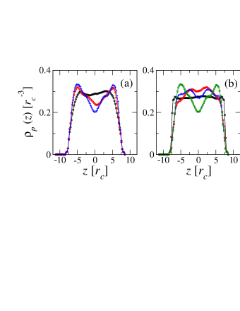
Figure 12: (a) Polymer density profile across the slit for the case of $\varphi=0.06$ and $N=100$ for varying values of the driving force: $f_{x}=0$ (squares), $f_{x}=0.02\epsilon/r_{c}$ (diamonds), and $f_{x}=0.04\epsilon/r_{c}$ (pluses). (b) Polymer density profile for the case of $\varphi=0.06$, $f_{x}=0.04\epsilon/r_{c}$, and chain length $N=5$ (circles), $N=20$ (diamonds), $N=50$ (pluses), and $N=100$ (squares).

The presence of a dip in the center-plane of the slit in Poiseuille flow implies a migration away from the very center of the slit. However, this can be accompanied by an increase in the depletion layer at the walls. Therefore an overall migration of the polymers cannot be merely inferred by merely looking at the depletion layer. We propose that the cross-stream migration issue can better be investigated through the second moment of the polymer volume fraction profile,

$$\langle z^{2}\rangle={\int_{-H}^{H}dzz^{2}\rho_{p}(z)}/{\int_{-H}^{H}dz\rho_{p}(z)}.$$ (16)

This is shown as a function of chain length, $N$, for all systems investigated in Fig. 13. A small $\langle z^{2}\rangle$ implies a general migration from the walls. This figure shows that in the absence of flow ($f_{x}=0$), $\langle z^{2}\rangle$ decreases as $N$ increases. This is due to the increase in the depletion layer as $N$ is increased. In the presence of flow, $\langle z^{2}\rangle$ decreases with increasing $N$ for small values of $\varphi$. However, for relatively large values of polymer volume fraction, $\langle z^{2}\rangle$ decreases with increasing $N$ for small values of $N$, but for large values of $N$, $\langle z^{2}\rangle$ increases with increasing $N$. Furthermore, Fig. 13 shows that for small values of $N$, the level of migration increases with increasing the driving force, $f_{x}$. However, for large values of $N$, more migration towards the wall is observed as $f_{x}$ is increased.

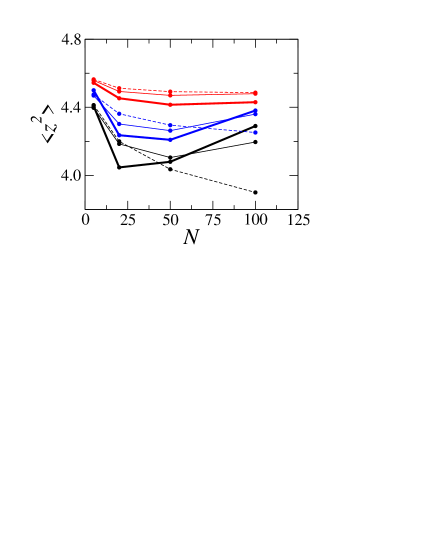
Figure 13: The second moment as calculated from Eq. (16) vs. chain length. Dashed lines correspond to $f_{x}=0$, thin solid lines correspond to $f_{x}=0.02\epsilon/r_{c}$,and thick solid lines correspond to $f_{x}=0.04\epsilon/r_{c}$. Black, blue and red lines correspond to $\varphi=0.06$, 0.12, and 0.24, respectively.

V Summary and Conclusions

We presented results obtained from a systematic computational study of flow of polymer solutions in nanoscale slit pores under the action of pressure gradient, using the dissipative particle dynamics approach. We found that while the flow of a simple fluid follows the Poiseuille-Hagen law, the flow of a polymer solution is characterized by a non-quadratic velocity profile and a lack of scaling with respect to both driving force and slit thickness that fits relatively well the generalized Poiseuille-Hagen law for non-Newtonian fluids with a power less than one. We also found that while the polymer chains are extended along the channel, the distribution of the three components of the radius of gyration is highly non-uniform across the channels.

The density profile of the polymers in the presence of pressure driven flow is also found to be non-uniform, exhibiting a local minimum in the center-plane and two off-center symmetric peaks. We found either a migration from or towards the wall depending on chain length, volume fraction and driving force. For relatively short chains and small polymer volume fractions, a migration away from the walls is observed. In this case, the level of migration is amplified as the chain length or driving force is increased. However, for longer chains a migration towards the wall is observed with the level of migration is increased as the chain length or the driving force is increased. For relatively concentrated polymer solutions, the level of migration is decreased.

It was argued earlier by Groot and Warren groot97 that DPD suffers from a low Schmidt number, ${\rm Sc}=\eta/\rho D_{0}\approx 1$, where $\eta$ is the viscosity, $\rho$ is the fluid density, and $D_{0}$ is the diffusivity of the solvent particles. In contrast a typical fluid has a Schmidt number of order 1000. A low Schmidt number implies that the particles diffuse as fast as momentum. Consequently, such an argument would lead us to conclude that the dynamics of polymer chains from DPD in a dilute solution will not follow the Zimm model. However, a recent extensive DPD study by us has shown that polymer chains in dilute solution correctly obey the Zimm model. Therefore, within DPD, the hydrodynamic interaction is well developed within the time scale of polymer motion. As noted recently by Peters peters04 , the Schmidt number in a coarse-grained model is in fact ill-defined, since in the Schmidt number, $D_{0}$ corresponds to the diffusion coefficient of single particle, not coarse-grained fluid elements. Our current findings provide further testimony to the effectiveness of the dissipative particle dynamics approach in simulating polymer flow in a variety of situations including in nano-channels.

References

- (1) U.S. Agarwal, A. Dutta, and R.A. Mashelkar, Chem. Eng. Sci. 49, 1693 (1994).
- (2) L. Fang, H. Hu, and R.G Larson, J. Rheol. 49, 127 (2005).
- (3) J. Han and H.G. Graighead, Science 288, 1026 (2000).
- (4) H. Müller-Mohnssen, D. Weiss, and A. Tippe, J. Rheol. 34, 223 (1990).
- (5) D. Ausserre, J. Edwards, J. Lecourtier, H. Hervet, and F. Rondelez, Europhys. Lett. 14, 33 (1991).
- (6) R.G. Horn, O.I. Vinogradova, M.E. Mackay, and N. Phan-Thien, J. Chem. Phys. 112, 6424 (2000).
- (7) P.J. Shrewsbury, S.J. Muller, and D. Liepmann, Biomed. Microdevices 3, 225 (2001).
- (8) X. Fan, N. Phan-Thien, N.T. Yong, X. Wu, and D. Xu, Phys. Fluids 15, 11 (2003).
- (9) N.J. Woo, E.S.G. Shaqfeh, and B. Khomami, J. Rheol. 48, 281 (2004).
- (10) N.J. Woo, E.S.G. Shaqfeh, and B. Khomami, J. Rheol. 48, 299 (2004).
- (11) R.M. Jendrejack, D.C. Schwartz, J.J. de Pablo, and M.D. Graham, J. Chem. Phys. 120, 2513 (2004).
- (12) H. Ma and M.D. Graham, J. Chem. Phys. 17, 083103 (2005).
- (13) O.B. Usta, A.J.C. Ladd, and J.E. Buttler, J. Chem. Phys. 122, 094902 (2005).
- (14) O.B. Usta, J.E. Buttler, and A.J.C. Ladd, Phys. Fluids 18, 031703 (2006).
- (15) R. Khare, M.D. Graham, and J.J. de Pablo, Phys. Rev. Lett. 96, 224505 (2006).
- (16) T.T. Perkins, D.E. Smith, and S. Chu, Science 276, 2016 (1997).
- (17) D.E. Smith, H.P. Babcock, and S. Chu, Science 283, 1724 (1999).
- (18) D.E. Smith and S. Chu, Science 281, 1335 (1998).
- (19) P.G. de Gennes, Scaling Concepts of Polymer Physics (Cornell University Press, Ithaca, 1979).
- (20) M. Ripoll, M.H. Ernst, and P. Español, J. Chem. Phys. 115, 7271 (2001).
- (21) W. Jiang, J. Huang, Y. Wang, and M. Laradji, submitted to J. Chem. Phys. (2006).
- (22) W. Jiang, Y. Wang, and M. Laradji (in preparation).
- (23) P.J. Hoogerbrugge and J.M.V.A. Koelman, Europhys. Lett. 19, 155 (1992).
- (24) P. Español and P. Warren, Europhys. Lett. 30, 191 (1995).
- (25) P. Español, Europhys. Lett. 40, 631 (1997).
- (26) I. Pagonabarraga, M.H.J. Hagen, and D. Frenkel, Europhys. Lett. 42, 377 (1998).
- (27) P. de Palma, P. Valentini, and M. Napolitano, Phys. Fluids 18, 027103 (2006).
- (28) X. Fan, N. Phan-Thien, S Chen, X. Wu, and T.Y. Ng, Phys. Fluids 18, 063102 (2006).
- (29) L.D. Landau and L.D. Lifshitz, Fluid Mechanics (Pergamon Press, Oxford, 1987).
- (30) M. Revenga, I. Zuniga, and P. Español, Int. J. Mod. Phys. C 9, 1319 (1998).
- (31) S.M. Willemsen, H.C.J. Hoefsloot, and P.D. Iedema, Int. J. Mod. Phys. C 11, 881 (2000).
- (32) J. Huang, Y. Wang, and M. Laradji, Macromolecules 39, 5546 (2006).
- (33) W.L. Wilkinson, Non-Newtonian Fluids: Fluid Mechanics, Mixing and Heat Transfer (Pergamon Press, 1960).
- (34) E.A. DiMarzio and C.M. Guttman, Macromolecules 3, 131 (1970).
- (35) R.D. Groot and P.B. Warren, J. Chem. Phys. 107, 4423 (1997).
- (36) E.A.J.F. Peters, Europhys. Lett. 66, 311 (2004).