Attractive Fermi gases with unequal spin populations in highly elongated traps

Abstract

We investigate two-component attractive Fermi gases with imbalanced spin populations in trapped one dimensional configurations. The ground state properties are determined within local density approximation, starting from the exact Bethe-ansatz equations for the homogeneous case. We predict that the atoms are distributed according to a two-shell structure: a partially polarized phase in the center of the trap and either a fully paired or a fully polarized phase in the wings. The partially polarized core is expected to be a superfluid of the FFLO type. The size of the cloud as well as the critical spin polarization needed to suppress the fully paired shell, are calculated as a function of the coupling strength.

Recent experimental studies of polarized Fermi gases near a Feshbach resonance have attracted a great deal of interest ketterle rice . Since a finite spin polarization destabilizes the Bardeen-Cooper-Schrieffer (BCS) s-wave superconductivity, these strongly interacting systems are indeed promising candidates to search for exotic pairing mechanisms.

So far, the experiments have mainly explored three-dimensional (3D) trapped configurations. The MIT data ketterle show that in the presence of a shallow trap the polarized Fermi gas phase-separates into three concentric shells: a fully paired superfluid core, an intermediate partially polarized normal shell and, finally, a fully polarized phase at the edge of the cloud. The Rice experiments have instead been performed on more anisotropic cigar-shaped configurations and the obtained measurements suggest a somewhat different scenario rice . A plausible explanation is that in the Rice experiments the applied trapping potential in the radial directions is tight enough that the gas cannot be considered as locally homogeneous and qualitatively new effects are seen which cannot be accounted for by the 3D local density approximation.

In this Letter, we study the limiting case where the radial confinement is so strong that only the lowest transverse mode is populated and the gas is kinematically one-dimensional (1D). We show that the ground state of the 1D polarized Fermi gas in a shallow axial trap exhibits a two-shell structure, in sharp contrast with the 3D case. Our analysis is based on the exact equation of state for a 1D homogeneous Fermi gas with arbitrary strong attractive interactions and the 1D local density approximation.

Strongly interacting 1D Fermi gases have already been investigated experimentally using ultracold atoms in optical lattices esslinger . The possibility to create spin imbalanced configurations opens new prospects to detect the Fulde-Ferrel-Larkin-Ovchinnikov (FFLO) state fulde note under clean experimental conditions. In particular, it was recently argued by Yang kunyang that the ground state of 1D homogeneous attractive Fermi gases with unequal spin populations is the 1D analogue of the FFLO state. For trapped configurations, this implies that the partially polarized phase of the 1D gas is a superfluid of the FFLO type and the experimentally measurable cloud sizes and density profiles provide indirect signatures of this unusual state. This is clearly exciting, because FFLO superconductivity has been of interest to condensed matter physicists for decades and, more recently, it has attracted the attention of the particle physics community casalbuoni .

Consider a two-component atomic Fermi gas in the presence of an axially symmetric harmonic potential

$$V_{trap}({\bf r})=\frac{1}{2}m\omega_{\perp}^{2}r_{\perp}^{2}+\frac{1}{2}m\omega_{z}^{2}z^{2},$$ (1)

where $m$ is the atom mass and $r_{\perp}=\sqrt{x^{2}+y^{2}}$. We require the anisotropy parameter $\lambda=\omega_{z}/\omega_{\perp}$ to be sufficiently small that only the lowest transverse mode is populated. At zero temperature, this condition implies that the Fermi energy $\epsilon_{F\uparrow}$ associated with the longitudinal motion of the majority $\uparrow$ component is much smaller than the distance between energy levels in the transverse direction, $\epsilon_{F\uparrow}\ll\hbar\omega_{\perp}$, or, equivalently, $\lambda\ll 1/N_{\uparrow}$. Under this assumption, Bergeman et al. olshani have shown that the scattering properties of atoms are well described by an effective 1D contact interaction $g_{1D}\delta(x)$, with

$$g_{1D}=\frac{2\hbar^{2}a_{3D}}{ma_{\perp}^{2}}\frac{1}{1-Aa_{3D}/a_{\perp}}\;,$$ (2)

where $a_{3D}$ is the 3D scattering length, $a_{\perp}=\sqrt{\hbar/m\omega_{\perp}}$ is the transverse oscillator length and $A=1.0326$. The effective 1D interaction is attractive, $g_{1D}<0$, if $1/a_{3D}<A/a_{\perp}$. By tuning the 3D scattering length near a Feshbach resonance, the coupling constant (2) can be changed adiabatically from the weakly interacting regime, $g_{1D}\rightarrow 0^{-}$, to the strong coupling limit, $g_{1D}\rightarrow-\infty$.

The effective 1D Hamiltonian $H_{1D}$ acting on the fermions is given by $H_{1D}=H_{1D}^{0}+\sum_{i=1}^{N}V_{ho}(z_{i})$, where $V_{ho}=m\omega_{z}^{2}z^{2}/2$ is the longitudinal trapping potential and

$$H_{1D}^{0}=-\frac{\hbar^{2}}{2m}\sum_{i=1}^{N}\frac{\partial^{2}}{\partial z_{i}^{2}}+g_{1D}\sum_{i=1}^{N_{\uparrow}}\sum_{j=1}^{N_{\downarrow}}\delta(z_{i}-z_{j}),$$ (3)

with $N=N_{\uparrow}+N_{\downarrow}$ being the total number of atoms. The Hamiltonian (3) is exactly soluble by Bethe’s ansatz gaudin .

Unpolarized 1D Fermi gases, in both homogeneous and trapped configurations, have been investigated in Ref.tokatly and Ref.alessio , as an exactly solvable model for the BEC-BCS crossover. The homogeneous case with a finite spin polarization has been recently studied in Ref.batchLONG . In the following we investigate the magnetic properties of spin polarized 1D attractive Fermi gases in harmonic traps at zero temperature. We first focus on the homogeneous case by setting $V_{ho}=0$. The effects of the axial confinement will be discussed later, using the 1D local density approximation (LDA).

For fixed values of the linear number densities $n_{\uparrow}=N_{\uparrow}/L$ and $n_{\downarrow}=N_{\downarrow}/L$, where $L$ is the size of the system, the ground state energy $E$ of $H_{1D}^{0}$ is given by gaudin

$$\frac{E}{L}=\frac{4\hbar^{2}}{ma_{1D}^{3}}\left[\int_{-B}^{B}(2\lambda^{2}-\frac{1}{2})\sigma(\lambda)d\lambda+\int_{-Q}^{Q}k^{2}\rho(k)dk\right].$$ (4)

The spectral functions $\sigma(\lambda),\rho(k)$ in Eq.(4) are solutions of the coupled integral equations gaudin

$$\sigma(\lambda) =\frac{1}{\pi}-\int_{-B}^{B}K_{1}(\lambda,\lambda^{\prime})\sigma(\lambda^{\prime})d\lambda^{\prime}-\int_{-Q}^{Q}K_{2}(\lambda,k)\rho(k)dk,$$ (5)

$$\rho(k) =\frac{1}{2\pi}-\int_{-B}^{B}K_{2}(\lambda,k)\sigma(\lambda)d\lambda,$$

where the kernels are given by $K_{1}(\lambda,\lambda^{\prime})=1/[\pi+\pi(\lambda^{\prime}-\lambda)^{2}]$ and $K_{2}(\lambda,k)=2/[\pi+4\pi(k-\lambda)^{2}]$. Here $B$ and $Q$ are non-negative numbers related to the number densities by $n_{\downarrow}a_{1D}=2\int_{-B}^{B}\sigma(\lambda)d\lambda$ and $n_{\uparrow}a_{1D}-n_{\downarrow}a_{1D}=2\int_{-Q}^{Q}\rho(k)dk$, respectively, and $a_{1D}=-2\hbar^{2}/mg_{1D}$ is the effective 1D scattering length. The coupling strength is controlled by the parameter $na_{1D}$, where $n=n_{\uparrow}+n_{\downarrow}$ is the total density: the weakly interacting case corresponds to $na_{1D}\gg 1$, whereas the strongly attractive regime is achieved for $na_{1D}\ll 1$.

The leading terms in the weak coupling expansion for the energy can be calculated by perturbation theory, yielding $E/L=\hbar^{2}\pi^{2}(n_{\downarrow}^{3}+n_{\uparrow}^{3})/6m-2\hbar^{2}n_{\uparrow}n_{\downarrow}/(ma_{1D})$. In the strongly interacting regime, corresponding to small values of $B$ and $Q$, we expand the spectral functions $\sigma(\lambda)$ and $\rho(k)$ around $\lambda=0$ and $k=0$, respectively, retaining up to quadratic terms. The coefficients of the expansion can be easily obtained from Eq.(5). From Eq.(4), we then obtain $E=E^{0}+\Delta E$, where the leading term is given by

$$\frac{E^{0}}{L}=-\epsilon_{B}n_{\downarrow}+\frac{\hbar^{2}\pi^{2}}{12m}n_{\downarrow}^{3}+\frac{\hbar^{2}\pi^{2}}{6m}(n_{\uparrow}-n_{\downarrow})^{3}$$ (6)

and $\Delta E=\hbar^{2}\pi^{2}a_{1D}[n_{\downarrow}^{3}(2n_{\uparrow}-n_{\downarrow})+8n_{\downarrow}(n_{\uparrow}-n_{\downarrow})^{3}]/12m$. The above result is in agreement with Ref.batchLONG . Equation (6) shows that in the strongly interacting regime the system is a mixture of a Tonks gas of $N_{\downarrow}$ diatomic molecules of mass $2m$ and binding energy $\epsilon_{B}=\hbar^{2}/ma_{1D}^{2}$, and an ideal Fermi gas formed by the unpaired $\uparrow$ fermions.

For a fixed value of the total density $n\equiv n_{\uparrow}+n_{\downarrow}$, the density difference $s\equiv n_{\uparrow}-n_{\downarrow}$ can vary in the range $0\leq s\leq n$. For $s=0$, the ground state of $H_{1D}^{0}$ is fully paired with a gap in the spin excitation spectrum alessio whereas in the opposite limit $s=n$, the system is a fully polarized gas of $\uparrow$ fermions. For $0<s<n$, the gas is partially polarized and it is expected to be a superfluid of the FFLO type kunyang .

From Eq.(4), we calculate the chemical potential $\mu\equiv\partial(E/L)/\partial n$ and the effective magnetic field $h\equiv\partial(E/L)/\partial s$, which are related to the chemical potentials $\mu_{\sigma}$ of the two components by $\mu=(\mu_{\uparrow}+\mu_{\downarrow})/2$ and $h=(\mu_{\uparrow}-\mu_{\downarrow})/2$. From Eq.(4) it follows that

$$\mu =\epsilon_{B}F_{\mu}(\tilde{n},\tilde{s}),$$ (7)

$$h =\epsilon_{B}F_{h}(\tilde{n},\tilde{s}),$$

where $F_{\mu}$ and $F_{h}$ are universal functions of the dimensionless number densities $\tilde{n}\equiv na_{1D}$ and $\tilde{s}\equiv sa_{1D}$. The energetic stability of the mixture in the partially polarized phase allows us to use $\mu$ and $h$ as new coordinates, since the Jacobian of the transformation (7) is positive pethick .

By setting $s=0$ in Eq.(7) we obtain the critical curve $\mu_{c}/\epsilon_{B}$ shown in Fig.1 and corresponding to the phase boundary with the fully paired phase. We see that $\mu_{c}$ diverges logarithmically for vanishing magnetic fields and decreases as $h$ increases, reaching its minimum value $\mu_{c}=-\epsilon_{B}/2$ for $h\rightarrow\epsilon_{B}/2^{-}$. The corresponding asymptotic behavior $\mu_{c}\simeq-h$ is plotted with a dashed line in the inset of Fig.1, where we have magnified the region of the phase diagram near the point O=$(\epsilon_{B}/2,-\epsilon_{B}/2)$. Similarly to what happens for the attractive Hubbard model woynarovich , the critical magnetic field $h_{c}=h(n,0)$ is related to the energy gap $\Delta$ in the spin sector for the unpolarized case by $h_{c}=\Delta/2$. Since $\Delta$ measures the strength of interactions, $h_{c}$ increases by decreasing the density $n$ (or, equivalently, the chemical potential $\mu$) reaching $h_{c}=\epsilon_{B}/2$ in the strongly attractive limit $\mu\rightarrow-\epsilon_{B}/2$, as shown in Fig.1.

By setting $s=n$ in Eq.(7) we obtain the second critical curve $\mu_{s}/\epsilon_{B}$ plotted in Fig.1 and corresponding to the phase boundary with the fully polarized phase. In this particular case, the saturation field $h(n,s=n)$ and the corresponding chemical potential $\mu_{s}=\mu(n,s=n)$ can be calculated in closed form from Eqs (4) and (5), yielding

$$h=2\epsilon_{B}[Q^{2}(1-\arctan(2Q)/\pi)+(2Q-\arctan(2Q)+\pi)/4\pi]$$ (8)

and $\mu_{s}=-h+2Q^{2}\epsilon_{B}$, where $Q=\pi na_{1D}/2$. In the weak coupling limit, corresponding to $h\gg\epsilon_{B}$, the chemical potential diverges as $\mu_{s}=h-4\sqrt{h\epsilon_{B}}/\pi+(4/\pi^{2}-1/2)\epsilon_{B}$ whereas in the strong coupling regime it approaches O as $\mu_{s}=-\epsilon_{B}/2+(2\sqrt{2}/3\pi\sqrt{\epsilon_{B}})(h-\epsilon_{B}/2)^{3/2}$. This latter behavior is also shown in the inset of Fig.1 with dashed line.

In Fig.1, the fully paired and the fully polarized phases are limited from below by a shaded area representing the vacuum state, i.e. the state of zero total density. For $h<\epsilon_{B}/2$, the minimum value of the chemical potential $\mu\equiv\mu_{v}$ is given by $\mu_{v}=-\epsilon_{B}/2$, whereas for $h>\epsilon_{B}/2$, we find $\mu_{v}=-h$, since $\mu+h=\mu_{\uparrow}$ is the chemical potential of the majority component.

We see from Fig.1 that for a fixed value of the magnetic field, only two phases are allowed for the 1D system: partially polarized and fully paired if $h<\epsilon_{B}/2$ or partially polarized and fully polarized if $h>\epsilon_{B}/2$. This is clearly different from the 3D case, where $\mu_{c}$ is an increasing function of the magnetic field mueller and thus all three phases are allowed for a given $h$.

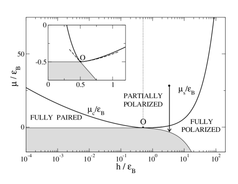
Figure 1: Ground state magnetic properties for the homogeneous system. The dotted vertical line corresponds to $h=\epsilon_{B}/2$. The arrow shows the trajectory of the local chemical potential in a trap. Inset: zoom of the phase diagram near the point O=$(\epsilon_{B}/2,-\epsilon_{B}/2)$: the asymptotic behaviors are shown with dashed lines.

The effects of a shallow harmonic potential $V_{ho}(z)$ can be taken into account via LDA, which is applicable provided the size of the cloud is large compared to the axial oscillator length $a_{z}=\sqrt{\hbar/m\omega_{z}}$, implying $N\gg 1$. Under this assumption, the density profiles $n_{\sigma}(r)$ for the two components $\sigma=\uparrow,\downarrow$ are obtained by imposing the local equilibrium condition $\mu_{\sigma}[n_{\uparrow}(z),n_{\downarrow}(z)]+V_{ho}(z)=\mu_{\sigma}^{0}$, where $\mu_{\sigma}[n_{\uparrow},n_{\downarrow}]$ are the corresponding chemical potentials of the homogeneous system and $\mu_{\sigma}^{0}$ are constants fixed by the normalization $N_{\sigma}=\int n_{\sigma}(z)dz$. This is equivalent to

$$\mu[n_{\uparrow}(z),n_{\downarrow}(z)] =\mu^{0}-V_{ho}(z),$$ (9)

$$h[n_{\uparrow}(z),n_{\downarrow}(z)] =h^{0},$$

where $\mu^{0},h^{0}=(\mu_{\uparrow}^{0}\pm\mu_{\downarrow}^{0})/2$. Equation (9) shows that the local mean chemical potential decreases by increasing the distance from the center of the trap while the local magnetic field remains constant throughout. In the phase diagram of Fig.1, this corresponds to follow the vertical line $h=h^{0}$ downwards starting from the point $\mu=\mu^{0}$, as shown by the arrow.

We immediately see that trapped gases with spin imbalanced components have a two-shell structure, with an inner partially polarized phase in the center of the trap. The outer shell is either fully paired, if $h^{0}<\epsilon_{B}/2$, or fully polarized, if $h^{0}>\epsilon_{B}/2$. Hence, the fully paired and the fully polarized phases are mutually exclusive in a trap. For the special case $h^{0}=\epsilon_{B}/2$, shown with dotted line in Fig.1, the partially polarized phase extends to the edge of the cloud.

In order to relate $\mu^{0},h^{0}$ to the total number $N\equiv N_{\uparrow}+N_{\downarrow}$ of atoms and the spin polarization $P\equiv(N_{\uparrow}-N_{\downarrow})/N$, we need to calculate the density profiles, starting from Eqs (4) and (9). The normalization conditions can be expressed in terms of the dimensionless chemical potential $\tilde{\mu}^{0}=\mu^{0}/\epsilon_{B}$ and the dimensionless densities $\tilde{n}$ and $\tilde{s}$, as

$$N\frac{a_{1D}^{2}}{a_{z}^{2}}=\sqrt{2}\int_{0}^{\tilde{\mu}_{v}}\frac{\tilde{n}(\tilde{\mu}^{0}-x)}{\sqrt{x}}dx,$$

$$(N_{\uparrow}-N_{\downarrow})\frac{a_{1D}^{2}}{a_{z}^{2}}=\sqrt{2}\int_{0}^{\tilde{\mu}_{v}}\frac{\tilde{s}(\tilde{\mu}^{0}-x)}{\sqrt{x}}dx,$$ (10)

where ${\tilde{\mu}_{v}}=\mu_{v}/\epsilon_{B}$. Equation (10) shows that, in the presence of the trap, the coupling strength is given by $Na_{1D}^{2}/a_{z}^{2}$, which is large in the weakly interacting regime and vanishes in the strongly attractive limit.

The condition $h^{0}=\epsilon_{B}/2$ yields the critical spin polarization $P=P_{c}$ needed to suppress the fully paired shell; for $P>P_{c}$ the outer shell is always fully polarized. In Fig.2 we plot the critical spin polarization as a function of the parameter $Na_{1D}^{2}/a_{z}^{2}$ (solid line). We see that $P_{c}$ increases going towards the strong coupling regime where it saturates to $P_{c}=0.2$. This value is surprisingly small compared to the critical polarization $P_{c}^{3D}\sim 0.77$ found ketterle in 3D Fermi gases at resonance $(a_{3D}\rightarrow\infty)$. The corresponding density profiles in the strongly attractive limit, where Eq.(6) holds, are given by $n_{\downarrow}(z)=(8m/\pi^{2}\hbar^{2})^{1/2}(\mu^{0}+\epsilon_{B}/2-V_{ho}(z))^{1/2}$, with $\mu^{0}+\epsilon_{B}/2=\hbar\omega_{z}N_{\downarrow}/2$, and $n_{\uparrow}(z)=n_{\downarrow}(z)+(2m/\pi^{2}\hbar^{2})^{1/2}(\mu^{0}+h^{0}-V_{ho}(z))^{1/2}$, with $\mu^{0}+h^{0}=(N_{\uparrow}-N_{\downarrow})\hbar\omega_{z}$. The inclusion of the next order correction $\Delta E$ yields $P_{c}=1/5(1-0.364\sqrt{Na_{1D}^{2}/a_{z}^{2}})$. This asymptotic behavior is shown in Fig.2 with dashed line.

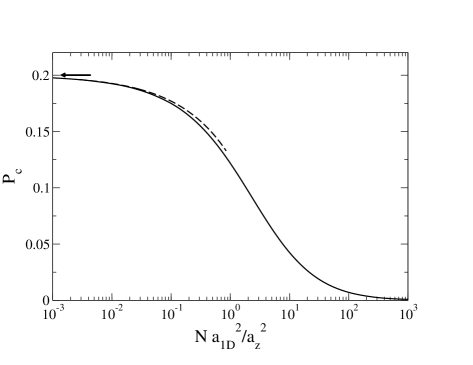
Figure 2: Critical spin polarization as a function of the interaction parameter $Na_{1D}^{2}/a_{z}^{2}$. The behavior in the strong coupling regime is shown with dashed line. The arrow corresponds to the asymptotic limit $P_{c}=0.2$.

For $P\neq P_{c}$, the cloud exhibits a two-shell structure, with the radius $R_{in}$ of the inner shell fixed by the condition $\mu^{0}-V_{ho}(R_{in})=\mu_{c}(h^{0})$, for $h^{0}<\epsilon_{B}/2$, and $\mu^{0}-V_{ho}(R_{in})=\mu_{s}(h^{0})$, otherwise. The size $R_{\uparrow}$ of the cloud, where the total density vanishes, is instead given by the condition $\mu^{0}-V_{ho}(R_{\uparrow})=\mu_{v}(h^{0})$. Both quantities are plotted in Fig.3 as a function of the spin polarization $P$ for different values of the parameter $Na_{1D}^{2}/a_{z}^{2}$. In the absence of interaction (top curve), we find $R_{\uparrow}=\sqrt{1+P}a_{z}N^{1/2}$ and $R_{in}=\sqrt{1-P}a_{z}N^{1/2}$, showing that $R_{\uparrow}(R_{in})$ increases (decreases) as $P$ increases. For finite interactions, we see that $R_{\uparrow}$ decreases as $P$ increases until $P=P_{c}$, and it increases for larger values of the spin polarization. In particular, in the strong coupling regime, we find $R_{\uparrow}=\sqrt{(1-P)/2}a_{z}N^{1/2}$ for $P\leq 1/5$, and $R_{\uparrow}=\sqrt{2P}a_{z}N^{1/2}$ for $P>1/5$. This non monotonic behavior is a signature of the outer shell. Indeed, an increase in the spin polarization implies that the radius of the density profile for the minority component decreases, as $N_{\downarrow}$ decreases. For $P<P_{c}$, the profiles for the two components match in the fully paired outer shell, and thus also $R_{\uparrow}$ decreases.

The inner radius (right panel) shows the opposite behavior: $R_{in}=0$ for zero spin polarization and it increases rapidly until $P=P_{c}$, where $R_{in}=R_{\uparrow}$ and the fully paired shell disappears. For higher values of the polarization, $R_{in}$ decreases and finally vanishes at $P=1$. In particular, in the strong coupling regime, we find $R_{in}=\sqrt{2P}a_{z}N^{1/2}$, for $P\leq 1/5$, and $R_{in}=\sqrt{(1-P)/2}a_{z}N^{1/2}$ for $P>1/5$.

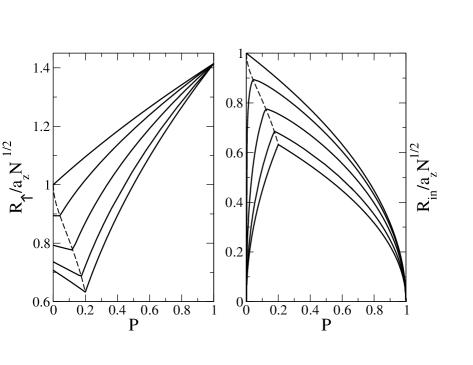
Figure 3: Size of the cloud (left) and radius of the inner shell (right) as a function of the spin polarization for different values of the parameter $Na_{1D}^{2}/a_{z}^{2}=\infty,10,1,0.1,0$. The non monotonic behavior is a signature of the two-shell structure.

The above scenario for a 1D polarized Fermi gas can be investigated in current experiments with ultracold atoms under a tight radial confinement, e.g. ⁴⁰K samples in an array of 1D tubes created with optical lattices esslinger . In order to reach a strongly degenerate regime, the thermal energy $k_{B}T$ should be small compared to the Fermi energy, implying $k_{B}T\ll N\hbar\omega_{z}$. This condition can be satisfied by taking the typical experimental parameters esslinger $\omega_{z}/2\pi\sim 250$ Hz for the axial frequency, mean number of particles (per tube) $N\sim 100$ and $T\sim 50$nK. The spin imbalance can be easily induced by a radio-frequency sweep and the density profiles measured by absorption imaging techniques.

In conclusion, we have presented an exact solution of an experimentally accessible 1D model of a polarized Fermi gas at arbitrary strong coupling. We have found that, differently from the 3D case, the trapped gas phase separates in a two-shell structure, with a FFLO superfluid core surrounded by either a fully paired or a fully polarized phase, depending on the value of the spin polarization. Experimental signatures of this novel and exotic state are a reduced value of the critical spin polarization $P_{c}$ and a non monotonic behavior of the size of the cloud as a function of the spin polarization.

We acknowledge fruitful discussions with N. Prokof’ev, S. Giorgini, W. Zwerger and G.V. Shlyapnikov. We are also grateful to Z. Idziaszek and G. Astrakharchik for useful suggestions on numerics. Finally, we want to thank G.V. Shlyapnikov for the kind hospitality at LPTMS (Orsay) during the preparation of this manuscript. This work was supported by the Ministero dell’Istruzione, dell’Universita’ e della Ricerca (M.I.U.R.).

References

- (1) M.W. Zwierlein et al, Science 311, 492 (2006); M.W. Zwierlein et al, Nature 442, 54 (2006); Y. Shin et al, Phys. Rev. Lett. 97, 030401 (2006).
- (2) G. B. Partridge et al, Science 311, 503 (2006); G. B. Partridge et al, Phys. Rev. Lett. 97, 190407 (2006).
- (3) H. Moritz et al, Phys. Rev. Lett. 94, 210401 (2005).
- (4) P. Fulde and A. Ferrell, Phys. Rev. 135, A550 (1964); A. Larkin and Y.N. Ovchinnikov, Zh. Eksp. Teor. Fiz. 47, 1136 (1964) [Sov. Phys. JETP 20, 762 (1965)].
- (5) The distinctive feature of the FFLO state is that the unpaired fermions induce an oscillatory behavior in the superconducting correlation function in the large distance limit .
- (6) K. Yang, Phys. Rev. B 63, 140511(R) (2001).
- (7) For a review, see R. Casalbuoni and G. Nardulli, Rev. Mod. Phys. 76, 263 (2004).
- (8) T. Bergeman, M.G. Moore, and M. Olshanii, Phys. Rev. Lett. 91, 163201 (2003).
- (9) M. Gaudin, La Fonction d’onde de Bethe, Masson (1983).
- (10) I. V. Tokatly, Phys. Rev. Lett. 93, 090405 (2004).
- (11) J. N. Fuchs, A. Recati, and W. Zwerger, Phys. Rev. Lett. 93, 090408 (2004).
- (12) N. Oelkers et al, J. Phys. A: Math. Gen. 39, 1073 (2006).
- (13) C.J. Pethick and H. Smith, Bose-Einstein Condensation in Dilute Gases, Cambridge University Press (2002).
- (14) T.B. Bahder and F. Woynarovich, Phys. Rev. B 33, 2114 (1986); F. Woynarovich and K. Penc, Z. Phys. B 85, 269 (1991).
- (15) T. N. De Silva and E. Mueller, Phys. Rev. A 73, 051602(R) (2006).