Theory of nonlinear optical spectroscopy of electron spin coherence in quantum dots

Abstract

We study in theory the generation and detection of electron spin coherence in nonlinear optical spectroscopy of semiconductor quantum dots doped with single electrons. In third-order differential transmission spectra, the inverse width of the ultra-narrow peak at degenerate pump and probe frequencies gives the spin relaxation time ($T_{1}$), and that of the Stoke and anti-Stoke spin resonances gives the effective spin dephasing time due to the inhomogeneous broadening ($T_{2}^{*}$). The spin dephasing time excluding the inhomogeneous broadening effect ($T_{2}$) is measured by the inverse width of ultra-narrow hole-burning resonances in fifth-order differential transmission spectra.

I Introduction

Electron spin coherence in semiconductor quantum dots (QDs) is a quantum effect to be exploited in emerging technologies such as spin-based electronics (spintronics) and quantum computation.Awschalom et al. (2002) The electron spin decoherence is a key issue for practical application of the electron spin freedom and is also of fundamental interest in mesoscopic physics and in quantum physics. The electron spin decoherence in QDs, however, is yet poorly characterized. By convention, the spin decoherence is classified into the longitudinal and the transverse parts, which correspond to the spin population flip and the Zeeman energy fluctuation processes and are usually characterized by the relaxation time $T_{1}$ and the dephasing time $T_{2}$, respectively. Most current experiments are carried out on ensembles of spins, composed of either many similar QDsGupta et al. (2002); Gurudev Dutt et al. (2005); Braun et al. (2005); Greilich et al. (2006) or many repetitions of (approximately) identical measurements on a single QD.Fujisawa et al. (2002); Elzerman et al. (2004); Johnson et al. (2005); Kroutvar et al. (2004); Bracker et al. (2005); Atatüre et al. (2006); Petta et al. (2005); Koppens et al. (2005, 2006) The ensemble measurements are subjected to the inhomogeneous broadening of the Zeeman energy which results from the fluctuation of the QD size, shape and compound composition (and in turn the electron $g$-factor) and from the random distribution of the local Overhauser field (due to the hyperfine interaction with nuclear spins in thermal states). The inhomogeneous broadening leads to an effective dephasing time $T_{2}^{*}$.Merkulov et al. (2002); Semenov and Kim (2003); Khaetskii et al. (2002) The three timescales characterizing the electron spin decoherence can differ by orders of magnitude usually in the order $T_{1}\gg T_{2}\gg T_{2}^{*}$. For example, in a typical GaAs QD at a low temperature ($\lesssim 4$ Kelvin) and under a moderate to strong magnetic field ($0.1\sim 10$ Tesla), the relaxation time $T_{1}$ can be in the order of milliseconds,Fujisawa et al. (2002); Elzerman et al. (2004); Johnson et al. (2005); Kroutvar et al. (2004); Bracker et al. (2005); Atatüre et al. (2006) the dephasing time $T_{2}$ is up to several microseconds,Petta et al. (2005); Koppens et al. (2006); Greilich et al. (2006) and the effective dephasing time $T_{2}^{*}$ can be as short as a few nanoseconds.Gurudev Dutt et al. (2005); Greilich et al. (2006); Petta et al. (2005); Koppens et al. (2005)

The issue is how to measure the characteristic times of electron spin decoherence in QDs. There have been many experiments both in opticsBraun et al. (2005); Kroutvar et al. (2004); Bracker et al. (2005); Atatüre et al. (2006) and in transportFujisawa et al. (2002); Elzerman et al. (2004); Johnson et al. (2005) which establish the spin relaxation time $T_{1}$ in QDs of different materials. The effective dephasing time $T_{2}^{*}$ is also measured for QD ensembles,Gupta et al. (2002); Gurudev Dutt et al. (2005); Greilich et al. (2006); Koppens et al. (2005); Petta et al. (2005) giving a lower bound of $T_{2}$. Spin echo in microwave ESR experiments is a conventional approach to measuring the spin decoherence time $T_{2}$ excluding the inhomogeneous broadening,Tyryshkin et al. (2003); Abe et al. (2004, 2005) which, however, is less feasible for III-V compound quantum dots due to the ultrafast timescales in such systems ($T_{2}\lesssim 10^{-6}$ sec and $T_{2}^{*}\lesssim 10^{-9}$ sec). Indeed, the remarkable spin echo experiments in coupled QDs done by the Marcus group are performed with rather long DC voltage pulses instead of instantaneous microwave pulses.Petta et al. (2005) Alternatively, picosecond optical pulses may be used to manipulate electron spins via Raman processesChen et al. (2003) and realize the spin echo, which, however, still need to overcome the difficulty of stabilizing and synchronizing picosecond pulses in microsecond time-spans. A recent experiment by Greilich et al also shows that the inhomogeneous broadening effect can be filtered out from the spin coherence mode-locked by a periodic train of laser pulses.Greilich et al. (2006)

In this paper, we will study the frequency-domain nonlinear optical spectroscopy as another approach to measuring the electron spin decoherence times. Particularly, the spin dephasing rate $T_{2}^{-1}$ is correlated to the width of ultra-narrow hole-burning peaks in fifth order differential transmission (DT) spectra. This hole-burning measurement of the spin dephasing time is analogous to the exploration of slow relaxation of optical coherence in atomic systems by the third-order hole-burning spectroscopy.Steel and Remillard (1987) Here the fifth order nonlinearity is needed because the creation of spin coherence by Raman processes involves at least two orders of optical field and hole-burning two more. The state-of-the-art spectroscopy already has the ultra-high resolution (much better than MHz-resolution) to resolve the slow spin decoherence in microsecond or even millisecond timescales.Steel and Rand (1985); Strickland et al. (2000); Ohno et al. (2004)

The organization of this paper is as follow: After this introductory section, Sec. II describes the model for QD system and the master-equation approach to calculating the nonlinear optical susceptibility. Sec. III presents the results and discussions. Sec. IV concludes this paper. The solution of the master equation in frequency domain is presented in Appendix A.

II Model and theory

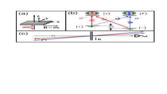
Figure 1: (Color online). Schematics of (a) the quantum dot, (b) the selection rules for optical transitions, and (c) the optical detection geometry.

The system to be studied is a semiconductor QD doped with a single electron. The geometry of the QD under an external magnetic field and optical excitation is shown in Fig. 1 (a) and (c). The QD is assumed of a shape with small thickness in the growth direction and relatively large radius in the lateral directions, as in the usual cases of fluctuation QDs and self-assembled QDs.Gurudev Dutt et al. (2005); Braun et al. (2005); Kroutvar et al. (2004); Bracker et al. (2005); Atatüre et al. (2006) To enable the generation and manipulation of the electron spin coherence through Raman processes, a magnetic field is applied along a lateral direction ($x$-axis). The propagation directions of the pump and probe laser beams are close to the growth direction ($z$-axis). The two electron spin states $|\pm\rangle$ are split by the magnetic field with Zeeman energy $\omega_{0}$. The strong confinement along the $z$-axis induces a large splitting between the heavy hole and the light hole states, thus the relevant exciton states are the ground trion states $|\tau\rangle$ and $|\bar{\tau}\rangle$ which consist of two electrons (including the doped one and one created by optical excitation) in the singlet spin state and one heavy hole in the spin state $|+3/2\rangle$ and $|-3/2\rangle$ (quantized along the $z$-axis with nearly zero Zeeman splitting), respectively. Similarly, we can also neglect the excitation of higher lying trions, bi-exciton and multi-exciton states since the energy of adding an exciton in each case is well separated from energy of the lowest trion states. The selection rules for the optical transitions are determined by the (approximate) conservation of the angular momentum along the growth direction so that a circularly polarized light with polarization $\sigma^{+}$ or $\sigma^{-}$ connects the two electron spin states to the trion state $|\tau\rangle$ or $\bar{\tau}\rangle$, respectively [see Fig. 1 (b)]. The relaxation processes in the system are parameterized by the exciton recombination rate $\Gamma_{1}$, the exciton dephasing rate $\Gamma_{2}$, the spin relaxation rate $T_{1}^{-1}$, and the spin dephasing rate $T_{2}^{-1}$. The inhomogeneous broadening leads to a random component $\epsilon$ to the Zeeman splitting: $\omega_{c}=\omega_{0}+\epsilon$, which is assumed of Gaussian distribution $g(\epsilon)=e^{-(\epsilon T_{2}^{*})^{2}/2}/(\sqrt{2\pi}/T_{2}^{*})$. The hole spin relaxation is neglected since it is extremely slow when the hole is confined in the trion states.Atatüre et al. (2006) The theory presented here can be extended straightforwardly to include the hole spin relaxation, the light-hole states, the hole mixing effect (which leads to the imperfection in the selection rules), the multi-exciton states, the inhomogeneous broadening of the trion states, and so on, but we expect no qualitative modification of the resonance features related to the electron spin coherence in the nonlinear optical spectra. For the interests of simplicity, we shall consider only $\sigma^{+}$-polarized optical field (extension to other polarization configurations may provide some flexibility for experiments and is trivial in the theoretical part). Thus the model is reduced to a $\Lambda$-type three-level system consisting of the two electron spin states $|\pm\rangle$ and the trion state $|\tau\rangle$. The $\Lambda$-type three-level model, in spite of its simplicity, is the basis of a wealth of physical effects including electromagnetically induced transparency,Harris et al. (1990) lasing without inversion,Harris (1989) and stimulated Raman adiabatic passage,Bergmann et al. (1998) and has been successfully applied to study transient optical signals of doped quantum dots.Gurudev Dutt et al. (2005); Economou et al. (2005)

The dynamics of the system is described in the density matrix formalism with $\rho_{\alpha,\beta}$ being the density matrix elements between the states $|\alpha\rangle$ and $|\beta\rangle$. The optical excitation and the relaxation are accounted for in the master equation as

$$\hskip-28.45274pt\partial_{t}\rho_{\tau,\pm} = -i({\mathcal{E}}_{g}\mp\omega_{c}/2-i\Gamma_{2})\rho_{\tau,\pm}$$ (1a)

$$-iE(t)\rho_{\tau,\tau}+iE(t)\rho_{\mp,\pm}+iE(t)\rho_{\pm,\pm},$$

$$\hskip-28.45274pt\partial_{t}\rho_{\tau,\tau} = -2\Gamma_{1}\rho_{\tau,\tau}+2\Im\left[E^{*}(t)\rho_{\tau,+}+E^{*}(t)\rho_{\tau,-}\right],$$ (1b)

$$\hskip-28.45274pt\partial_{t}\rho_{\pm,\pm} = -\left(p_{\mp}\rho_{\pm,\pm}-p_{\pm}\rho_{\mp,\mp}\right)/T_{1}+\Gamma_{1}\rho_{\tau,\tau}$$ (1c)

$$-{2}\Im\left[E^{*}(t)\rho_{\tau,\pm}\right],$$

$$\hskip-28.45274pt\partial_{t}\rho_{\pm,\mp} = \Gamma_{1}\rho_{\tau,\tau}-i(\pm\omega_{c}-i/T_{2})\rho_{\pm,\mp}$$ (1d)

$$+iE^{*}(t)\rho_{\tau,\mp}-iE(t)\rho^{*}_{\tau,\pm},$$

where ${\mathcal{E}}_{g}$ is the energy gap, and $p_{\pm}$ is the equilibrium population of the spin states in absence of the optical excitation, and the optical field $E(t)=\sum_{j}E_{j}e^{-i\Omega_{j}t}$ contains different frequency components. The transition dipole moment is understood to be absorbed into the field quantities. In the rotating wave reference frame, the energy gap ${\mathcal{E}}_{g}$ is set to be zero and the optical frequencies $\Omega_{j}$ are measured from the gap. The first term in the righthand side of Eq. (1d) is the spin coherence generated by spontaneous emission,Economou et al. (2005); Javanainen (1992); Shabaev et al. (2003) which has been demonstrated in time-domain experiments with significant effects on spin beats.Gurudev Dutt et al. (2005) We will show that it produces extra resonances in fifth-order DT spectra.

To calculate the nonlinear optical susceptibility, the master equation is obtained in the frequency-domain (as given in Appendix A). With the spectrum of the optical field given by $E(\Omega)=\sum_{j}2\pi E_{j}\delta\left(\Omega-\Omega_{j}\right)$, the density matrix can be expanded as

$$\rho_{\alpha,\beta}(\Omega) = \sum_{j,\ldots,k;m,\ldots,l}2\pi E_{j}\cdots E_{k}E_{m}^{*}\cdots E_{l}^{*}$$ (2)

$$\times\rho_{\alpha,\beta}^{(j\cdots k\bar{m}\cdots\bar{l})}\delta\left(\Omega-\Omega_{j\cdots k\bar{m}\cdots\bar{l}}\right),$$

where $\Omega_{j\cdots k\bar{m}\cdots\bar{l}}\equiv\Omega_{j}+\cdots+\Omega_{k}-(\Omega_{m}+\cdots+\Omega_{l})$. The derivation of the density matrix component $\rho^{(j\cdots k\bar{m}\cdots\bar{l})}$ up to the fifth order is lengthy but straightforward. The final result is averaged with the inhomogeneous broadening distribution $g(\epsilon)$.

III Results and discussions

The linear optical susceptibility is given by

$$\rho^{(j)}=\int\frac{g(\epsilon)}{\Omega_{j}-{\mathcal{E}}_{g}\pm\omega_{c}/2+i\Gamma_{2}}d\epsilon.$$ (3)

In fluctuation GaAs QDs, the exciton dephasing is much faster than the effective spin dephasing due to the inhomogeneous broadening ($\Gamma_{2}^{-1}\lesssim 0.1$ ns $\ll T_{2}^{*}\sim 10$ ns),Gurudev Dutt et al. (2005) so the resonance width in linear optical spectra is usually dominated by the trion state broadening, revealing little information about the spin decoherence.

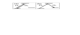
Figure 2: Schematics of Raman processes generating (a) the spin population and (b) the off-diagonal spin coherence.

In third-order optical response, the population and off-diagonal coherence of the electron spin are generated by the Raman processes

$$\hskip-28.45274pt\rho_{\pm,\pm}\stackrel{{\scriptstyle E_{2}}}{{\longrightarrow}}\rho^{(2)}_{\tau,\pm}\stackrel{{\scriptstyle E_{1}^{*}}}{{\longrightarrow}}\rho^{(2\bar{1})}_{\pm,\pm}\propto\left(\Omega_{2\bar{1}}+i/T_{1}\right)^{-1},$$ (4a)

$$\hskip-28.45274pt\rho_{\pm,\pm}\stackrel{{\scriptstyle E_{2}}}{{\longrightarrow}}\rho^{(2)}_{\tau,\pm}\stackrel{{\scriptstyle E_{1}^{*}}}{{\longrightarrow}}\rho^{(2\bar{1})}_{\mp,\pm}\propto\left(\Omega_{2\bar{1}}\pm\omega_{c}+i/T_{1}\right)^{-1},$$ (4b)

corresponding to the illustrations in Fig. 2 (a) and (b), respectively. Another optical field with frequency $\Omega_{1}$ brings the second order spin coherence into the third order optical coherence $\rho^{(21\bar{1})}_{\tau,\pm}$. The DT spectrum as a function of the pump frequency $\Omega_{1}$ and the probe frequency $\Omega_{2}$ is

$$S_{\rm DT}\left(\Omega_{2},\Omega_{1}\right)\propto-\Im\left[\rho^{(21\bar{1})}_{\tau,+}+\rho^{(21\bar{1})}_{\tau,-}\right],$$ (5)

which presents ultra-narrow resonances around $\Omega_{2\bar{1}}=\pm\omega_{0}$ and $\Omega_{2\bar{1}}=0$, with resonance width $T_{2}^{-1}$ and $T_{1}^{-1}$, related to the spin population and off-diagonal coherence in Eq. (4a) and (4b), respectively. Such resonances are shown in Fig. 3. Thus the spin dephasing time $T_{2}$ and relaxation time $T_{1}$ are measured. But when the inhomogeneous broadening is included, since usually $T_{2}\gg T_{2}^{*}$, the Stoke and anti-Stoke Raman resonances at $\Omega_{2\bar{1}}=\pm\omega_{0}$ will be smeared to be a peak resembling the inhomogeneous broadening distribution as

$$\int\rho^{(2\bar{1})}_{\pm,\mp}g(\epsilon)d\epsilon\sim-i\pi g\left(\Omega_{2\bar{1}}\mp\omega_{0}\right).$$ (6)

The effect of the inhomogeneous broadening is clearly seen in Fig. 3. So in usual cases, the third-order DT spectra measure the $T_{2}^{*}$ instead of the $T_{2}$. The resonance at degenerate pump and probe frequencies ($\Omega_{2\bar{1}}=0$) is related to the spin population and is immune to the random distribution of the electron Zeeman energy. So the spin relaxation time $T_{1}$ can be deduced from the third order DT spectra, regardless of the inhomogeneous broadening.

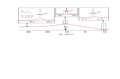
Figure 3: (Color online). Third-order DT spectra of QDs doped with single electrons. The parameters are chosen such that the Zeeman energy $\omega_{0}=20$ $\mu$eV, the spin population $p_{\pm}=0.5$, the pump frequency $\Omega_{1}={\mathcal{E}}_{g}-10.5$ $\mu$eV, $\Gamma_{1}=5$ $\mu$eV ($\Gamma_{1}^{-1}\approx 0.12$ ns), $\Gamma_{2}=6$ $\mu$eV ($\Gamma_{2}^{-1}\approx 0.1$ ns), $T_{1}=100$ ns, $T_{2}=100$ ns, and $T_{2}^{*}=10$ ns or artificially set to be $\infty$ for the solid and dotted lines, respectively. The insets are enlarged plots showing details of the resonances.

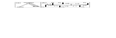
Figure 4: (a) Schematics for a fourth-order optical process that generate spin coherence with a double resonance structure. (b) The Feynman diagram for the fifth order optical response involving the spontaneous emission, in which the optical field and the vacuum field are represented by the wavy arrows and the dotted arrow, respectively.

To measure the spin dephasing time excluding the inhomogeneous broadening effect, the fifth order nonlinearity can be used. In the fifth order optical response, the spin coherence in the fourth order of optical field has very rich resonance structures. For instance, a double resonance like

$$\rho^{(43\bar{2}\bar{1})}_{+,-}\sim\left(\Omega_{3\bar{1}}-\omega_{c}+i/T_{2}\right)^{-1}\left(\Omega_{43\bar{2}\bar{1}}-\omega_{c}+i/T_{2}\right)^{-1},$$ (7)

arises from the excitation pathway

$$\rho_{-,-}\stackrel{{\scriptstyle E_{3}}}{{\longrightarrow}}\rho^{(3)}_{\tau,-}\stackrel{{\scriptstyle E_{1}^{*}}}{{\longrightarrow}}\rho^{(3\bar{1})}_{+,-}\stackrel{{\scriptstyle E_{4}}}{{\longrightarrow}}\rho^{(43\bar{1})}_{\tau,-}\stackrel{{\scriptstyle E_{2}^{*}}}{{\longrightarrow}}\rho^{(43\bar{2}\bar{1})}_{+,-},$$ (8)

as depicted in Fig. 4 (a). The double resonance will manifest itself in a two-dimensional DT spectrum as an ultra-narrow peak at $\Omega_{3\bar{1}}=\Omega_{43\bar{2}{1}}=\omega_{c}$ with width $\sim T_{2}^{-1}$. When the inhomogeneous broadening is included, the ultra-narrow resonance will be smeared into a broadened peak along the direction $\Omega_{3\bar{1}}=\Omega_{43\bar{2}{1}}$ with width $\sim 1/T_{2}^{*}$. But in the perpendicular direction (defined by $\Omega_{3\bar{1}}=-\Omega_{43\bar{2}{1}}$), the peak width remains unchanged. So when $\Omega_{43\bar{2}{1}}$ is fixed around $\omega_{0}$ and $\Omega_{3\bar{1}}$ is scanned, or vice versa, the DT spectrum will present a sharp peak whose width measures the inverse spin dephasing time $T_{2}^{-1}$. This peak has the character of hole-burning: The first frequency difference acts just as a selection of QDs with Zeeman energy $\omega_{c}=\Omega_{43\bar{2}\bar{1}}$ from the inhomogeneously broadened ensemble. The hole-burning resonance resulting from the excitation pathway in Eq. (8), however, emerges together with the resonance associated with the spin population $(\Omega_{4\bar{2}}+i/T_{1})^{-1}$ as given in Eq. (4a). To avoid the complication of mixing two types of resonance structures, we would rather make use another mechanism for spin coherence generation, namely, the spontaneous emission that connects the trion state to the two spin states through the vacuum field [related to the first term in the righthand side of Eq.(1d)].Gurudev Dutt et al. (2005); Economou et al. (2005); Javanainen (1992); Shabaev et al. (2003)

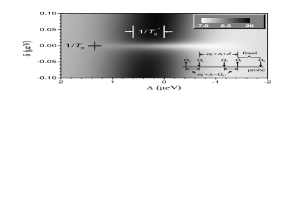
Figure 5: Contour plot of the fifth-order DT spectrum of the QDs as a function of $\Delta\equiv\Omega_{43\bar{2}{1}}-\omega_{0}$ and $\delta\equiv\Omega_{1\bar{3}}-\Omega_{43\bar{2}{1}}$. The probe frequency is fixed to be $\Omega_{4}=22$ $\mu$eV, the pump frequency $\Omega_{1}$ is fixed at $9$ $\mu$eV, and the other three pump frequencies are scanned with $\Omega_{53\bar{2}\bar{1}}=0$ (which makes $\Omega_{1\bar{5}}=\Omega_{3\bar{2}}=\omega_{0}+\Delta-\Omega_{4\bar{1}}$ and $\Omega_{1\bar{3}}=\Omega_{5\bar{2}}=\omega_{0}+\Delta+\delta$, as indicated in the inset). The Zeeman energy $\omega_{0}=20$ $\mu$eV, the spin population $p_{\pm}=0.5$, and the relaxation rates are such that $\Gamma_{1}=5$ $\mu$eV ($\Gamma_{1}^{-1}\approx 0.12$ ns), $\Gamma_{2}=6$ $\mu$eV ($\Gamma_{2}^{-1}\approx 0.1$ ns), $T_{1}=100$ ns, $T_{2}=100$ ns, and $T_{2}^{*}=1$ ns.

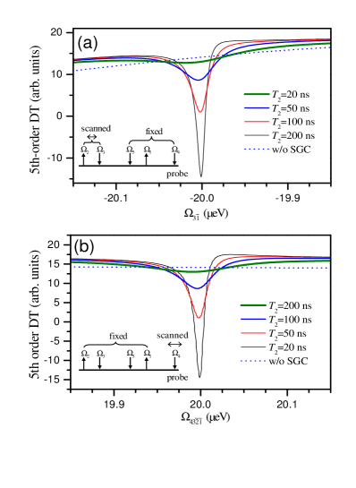
Figure 6: (Color online) (a) The sectioned plot of Fig. 5 with $\Delta=0$ (i.e., $\Omega_{43\bar{2}\bar{1}}=\omega_{0}$). (b) The fifth-order DT signal as a function of the probe frequency with pump frequencies fixed to be such that $\Omega_{1}=9$ $\mu$eV, $\Omega_{5}=2$ $\mu$eV, and $\Omega_{1\bar{3}}=\Omega_{5\bar{2}}=\omega_{0}=20$ $\mu$eV. In both figures, the spin dephasing time $T_{2}=20$, 50, 100 and 200 ns for the solid curves from top to bottom, and the dotted line is calculated with the spontaneously generated spin coherence artificially switched off (for $T_{2}=100$ ns). The parameters are the same as in Fig. 5.

The generation of spin coherence in the fifth order optical response involving the spontaneous emission can take a quantum pathway like

$$\rho_{-,-}\stackrel{{\scriptstyle E_{3}}}{{\longrightarrow}}\rho^{(3)}_{\tau,-}\stackrel{{\scriptstyle E_{1}^{*}}}{{\longrightarrow}}\rho^{(3\bar{1})}_{+,-}\stackrel{{\scriptstyle E_{4}}}{{\longrightarrow}}\rho^{(43\bar{1})}_{\tau,-}\stackrel{{\scriptstyle E_{2}^{*}}}{{\longrightarrow}}\rho^{(43\bar{2}\bar{1})}_{\tau,\tau}\stackrel{{\scriptstyle\Gamma_{1}}}{{\dashrightarrow}}\rho^{(43\bar{2}\bar{1})}_{-,+},$$ (9)

where the last step is the spontaneous emission. This optical process is illustrated by the Feynman diagram in Fig. 4 (b). The spin coherence generated by the spontaneous emission and that by optical excitation can have opposite spin indices [$\rho^{(3\bar{1})}_{+,-}\longrightarrow\rho^{(43\bar{2}\bar{1})}_{-,+}$], which is impossible in quantum pathways without the spontaneous emission [as can be seen from Fig. 4 (a)]. Thus the double resonance becomes

$$\rho^{(43\bar{2}\bar{1})}_{-,+}\sim\frac{\Gamma_{1}/\left(\Omega_{43\bar{2}\bar{1}}+i2\Gamma_{1}\right)}{\left(\Omega_{3\bar{1}}+\omega_{c}+iT_{2}^{-1}\right)\left(\Omega_{43\bar{2}\bar{1}}-\omega_{c}+iT_{2}^{-1}\right)},$$ (10)

which is well separated from the spin population resonance. The spectrum is measured by fixing $\Omega_{43\bar{2}{1}}$ to be the hole-burning frequency $\omega_{0}+\Delta$ with $\Delta\lesssim 1/T_{2}^{*}$ and fine-tuning $\Omega_{1\bar{3}}$ to be $\Omega_{43\bar{2}{1}}+\delta$. As shown in the inset of Fig. 5, the optical frequencies can be configured such that $\Omega_{4}$ and $\Omega_{1}$ are fixed, $\Omega_{3}$ are red-shifted by $\omega_{0}+\Delta+\delta$ from $\Omega_{1}$, and $\Omega_{5}$ and $\Omega_{2}$ are red-shifted by $\omega_{0}+\Delta-\Omega_{4\bar{1}}$ from $\Omega_{1}$ and $\Omega_{3}$, respectively. Thus the fifth-order optical response $\rho^{(543\bar{2}\bar{1})}_{\tau,\pm}$ oscillates at the probe frequency $\Omega_{4}$, which enables the signal to be measured in the DT setup instead of six-wave mixing ones. We note that the resonance due to the spin population $\sim\left(\Omega_{53\bar{2}\bar{1}}+i/T_{1}\right)^{-1}$ contributes only a constant background since $\Omega_{53\bar{2}\bar{1}}\equiv 0$ in the above frequency configuration. As shown in Fig. 5 which plots the fifth order DT spectrum as a function of $\Delta\equiv\Omega_{43\bar{2}\bar{1}}-\omega_{0}$ and the fine tuning $\delta\equiv\Omega_{1\bar{3}}-\Omega_{43\bar{2}\bar{1}}$, a very narrow hole in the spectrum as a function of $\Omega_{3\bar{1}}$ is burnt around $\Omega_{43\bar{2}\bar{1}}$, with width given by $T_{2}^{-1}$. Along the direction $\Omega_{3\bar{1}}=-\Omega_{43\bar{2}\bar{1}}$ ($\delta=0$), the resonance is extended by the inhomogeneous broadening as expected. Sectioned plots of the DT signal with fixed $\Delta$ are shown in Fig. 6 (a) for various spin dephasing time. The resonance width is given by the spin dephasing rate, demonstrating unambiguously that the $T_{2}$ is measured by the hole burning effect. The hole burning resonance can also be detected by varying the probe frequency with the pump frequencies fixed, as demonstrated in Fig. 6 (b). The role of the spontaneous emission-generated spin coherence is verified by the absence of the ultra-narrow resonance with artificial switch-off of the relevant term in Eq. (1d).

IV Conclusions

The spin coherence can be generated and detected in nonlinear optical spectroscopy of quantum dots doped with single electrons, which is studied in this paper up to the fifth order nonlinearity with a $\Lambda$-type three-level model. The electron spin coherence is generated by the optical field through Raman processes as well as by spontaneous emission of the trion. The spin population and off-diagonal coherence demonstrate themselves in third-order differential transmission spectra as ultra-narrow resonances. The inhomogeneous broadening smears out the sharp Stoke and anti-Stoke peaks related to the off-diagonal spin coherence. Thus the spin relaxation time $T_{1}$ and the effective dephasing time $T_{2}^{*}$ are measured by the third-order spectra. In the fifth-order optical response, the generation of the spin coherence by both second- and fourth-order optical processes leads to double resonance structures in two-dimensional DT spectra, which are smeared by the inhomogeneous broadening along one direction in the frequency space but presents ultra-narrow hole-burning resonances along the perpendicular direction. So the spin dephasing time $T_{2}$ is measured as the inverse width of the hole burning peak. The spontaneous emission-generated spin coherenceGurudev Dutt et al. (2005); Economou et al. (2005) is useful to produce hole burning resonances well separated from the spin-population resonances in the fifth-order spectra. The frequencies of the optical field can be configured properly to enable the detection of the signal in the DT setup instead of the multi-wave mixing ones. In practice, the pump and probe frequencies may be generated from a single continuous-wave laser source by, e.g., acousto-optical modulation.Ohno et al. (2004) Since the ultra-narrow hole burning peaks are rather insensitive to the global shift of the laser frequencies and variation of the hole-burning frequency, non-stabilized laser sources may be used to resolve the slow spin decoherence.Ohno et al. (2004)

Appendix A Solution of the master equation

The master equation in Eq. (1) can be solved in the frequency domain by Fourier transformation to be

$${\rho}_{\tau,\pm}(\Omega)=\int\frac{-E(\Omega-\omega){\rho}_{\pm,\pm}(\omega)-E(\Omega-\omega){\rho}_{\mp,\pm}(\omega)+E(\Omega-\omega){\rho}_{\tau,\tau}(\omega)}{\Omega-{\mathcal{E}}_{g}{\pm}\omega_{c}/2+i\Gamma_{2}}\frac{d\omega}{2\pi},$$ (11a)

$${\rho}_{\tau,\tau}(\omega)=\sum_{\pm}\int\frac{+E^{*}(\Omega-\omega){\rho}_{\tau,\pm}(\Omega)-E(\Omega+\omega){\rho}^{*}_{\tau,\pm}(\Omega)}{\omega+i2\Gamma_{1}}\frac{d\Omega}{2\pi},$$ (11b)

$${\rho}_{\pm,\pm}(\omega)={p_{\pm}}2\pi\delta(\omega)-\left(\omega+i\Gamma_{1}+ip_{\pm}/T_{1}\right)\int\frac{E^{*}(\Omega-\omega){\rho}_{\tau,\pm}(\Omega)-E(\Omega+\omega){\rho}^{*}_{\tau,\pm}(\Omega)}{\left(\omega+i/T_{1}\right)\left(\omega+i2\Gamma_{1}\right)}\frac{d\Omega}{2\pi}$$

$$\phantom{{\rho}_{\pm,\pm}(\omega)={p_{\pm}}2\pi\delta(\omega)}+\left(i\Gamma_{1}-ip_{\pm}/T_{1}\right)\int\frac{E^{*}(\Omega-\omega){\rho}_{\tau,\mp}(\Omega)-E(\Omega+\omega){\rho}^{*}_{\tau,\mp}(\Omega)}{\left(\omega+i/T_{1}\right)\left(\omega+i2\Gamma_{1}\right)}\frac{d\Omega}{2\pi},$$ (11c)

$${\rho}_{+,-}(\omega)=\frac{i{\Gamma_{1}}{\rho}_{\tau,\tau}(\omega)}{\omega-\omega_{c}+i/T_{2}}+\int\frac{-E^{*}(\Omega-\omega){\rho}_{\tau,-}(\Omega)+E(\Omega+\omega){\rho}^{*}_{\tau,+}(\Omega)}{\omega-\omega_{c}+i/T_{2}}\frac{d\Omega}{2\pi}.$$ (11d)

References

- Awschalom et al. (2002) D. D. Awschalom, D. Loss, and N. Samarth, eds., Semiconductor spintronics and quantum computation (Springer, New York, 2002).
- Gupta et al. (2002) J. A. Gupta, D. D. Awschalom, A. L. Efros, and A. V. Rodina, Phys. Rev. B 66, 125307 (2002).
- Gurudev Dutt et al. (2005) M. V. Gurudev Dutt, J. Cheng, B. Li, X. Xu, X. Li, P. R. Berman, D. G. Steel, A. S. Bracker, D. Gammon, S. E. Economou, et al., Phys. Rev. Lett. 94, 227403 (2005).
- Braun et al. (2005) P. Braun, X. Marie, L. Lombez, B. Urbaszek, T. Amand, P. Renucci, V. Kalevich, K. Kavokin, O. Krebs, P. Voisin, et al., Phys. Rev. Lett. 94, 116601 (2005).
- Greilich et al. (2006) A. Greilich, D. R. Yakovlev, A. Shabaev, A. L. Efros, I. A. Yugova, R. Oulton, V. Stavarache, D. Reuter, A. Wieck, and M. Bayer, Science 313, 341 (2006).
- Fujisawa et al. (2002) T. Fujisawa, D. G. Austing, Y. Tokura, Y. Hirayama, and S. Tarucha, Nature 419, 278 (2002).
- Elzerman et al. (2004) J. M. Elzerman, R. Hanson, L. H. Willems van Beveren, B. Witkamp, L. M. K. Vandersypen, and L. P. Kouwenhoven, Nature 430, 431 (2004).
- Johnson et al. (2005) A. C. Johnson, J. R. Petta, J. M. Taylor, A. Yacoby, M. D. Lukin, C. M. Marcus, M. P. Hanson, and A. C. Gossard, Nature 435, 925 (2005).
- Kroutvar et al. (2004) M. Kroutvar, Y. Ducommun, D. Heiss, M. Bichler, D. Schuh, D. Abstreiter, and J. J. Finley, Nature 432, 81 (2004).
- Bracker et al. (2005) A. S. Bracker, E. A. Stinaff, D. Gammon, M. E. Ware, J. G. Tischler, A. Shabaev, A. L. Efros, D. Park, D. Gershoni, V. L. Korenev, et al., Phys. Rev. Lett. 94, 047402 (2005).
- Atatüre et al. (2006) M. Atatüre, J. Dreiser, A. Högele, K. Karrai, and A. Imamoglu, Science 312, 551 (2006).
- Petta et al. (2005) J. R. Petta, A. C. Johnson, J. M. Taylor, E. A. Laird, A. Yacoby, M. D. Lukin, C. M. Marcus, M. P. Hanson, and A. C. Gossard, Science 309, 2180 (2005).
- Koppens et al. (2005) F. H. L. Koppens, J. A. Folk, J. M. Elzerman, R. Hanson, L. H. W. van Beveren, I. T. Vink, H. P. Tranitz, W. Wegscheider, L. P. Kouwenhoven, and L. M. K. Vandersypen, Science 309, 1346 (2005).
- Koppens et al. (2006) F. H. L. Koppens, C. Buizert, K. J. Tielrooij, I. T. Vink, K. C. Nowack, T. Meunier, L. P. Kouwenhoven, and L. M. K. Vandersypen, Nature 442, 766 (2006).
- Merkulov et al. (2002) I. A. Merkulov, A. L. Efros, and M. Rosen, Phys. Rev. B 65, 205309 (2002).
- Semenov and Kim (2003) Y. G. Semenov and K. W. Kim, Phys. Rev. B 67, 073301 (2003).
- Khaetskii et al. (2002) A. V. Khaetskii, D. Loss, and L. Glazman, Phys. Rev. Lett. 88, 186802 (2002).
- Tyryshkin et al. (2003) A. M. Tyryshkin, S. A. Lyon, A. V. Astashkin, and A. M. Raitsimring, Phys. Rev. B 68, 193207 (2003).
- Abe et al. (2004) E. Abe, K. M. Itoh, J. Isoya, and S. Yamasaki, Phys. Rev. B 70, 033204 (2004).
- Abe et al. (2005) E. Abe, J. Isoya, and K. M. Itoh, J. Supercond. 18, 157 (2005).
- Chen et al. (2003) P. Chen, C. Piermarocchi, L. J. Sham, D. Gammon, and D. G. Steel, Phys. Rev. B 69, 075320 (2003).
- Steel and Remillard (1987) D. G. Steel and J. T. Remillard, Phys. Rev. A 36, 4330 (1987).
- Steel and Rand (1985) D. G. Steel and S. C. Rand, Phys. Rev. Lett. 55, 2285 (1985).
- Strickland et al. (2000) N. M. Strickland, P. B. Sellin, Y. Sun, J. L. Carlsten, and R. L. Cone, Phys. Rev. B 62, 1473 (2000).
- Ohno et al. (2004) S. Ohno, T. Ishii, T. Sonehara, A. Koreeda, and S. Saikan, J. Luminescence 107, 298 (2004).
- Harris et al. (1990) S. E. Harris, J. E. Field, and A. Imamoğlu, Phys. Rev. Lett. 64, 1107 (1990).
- Harris (1989) S. E. Harris, Phys. Rev. Lett. 62, 1033 (1989).
- Bergmann et al. (1998) K. Bergmann, H. Theuer, and B. W. Shore, Rev. Mod. Phys. 70, 1003 (1998).
- Economou et al. (2005) S. E. Economou, R. B. Liu, L. J. Sham, and D. G. Steel, Phys. Rev. B 71, 195327 (2005).
- Javanainen (1992) J. Javanainen, Europhys. Lett. 17, 407 (1992).
- Shabaev et al. (2003) A. Shabaev, A. L. Efros, D. Gammon, and I. A. Merkulov, Phys. Rev. B 68, 201305(R) (2003).