Construction of a giant vortex state in a trapped Fermi system

Abstract

A superfluid atomic Fermi system may support a giant vortex if the trapping potential is anharmonic. In such a potential, the single-particle spectrum has a positive curvature as a function of angular momentum. A tractable model is put up in which the lowest and next lowest Landau levels are occupied. Different parameter regimes are identified and characterized. Due to the dependence of the interaction on angular momentum quantum number, the Cooper pairing is at its strongest not only close to the Fermi level, but also close to the energy minimum. It is shown that the gas is superfluid in the interior of the toroidal density distribution and normal in the outer regions. Furthermore, the pairing may give rise to a localized density depression in configuration space.

I Introduction

Among the features that distinguish a superfluid from a normal fluid is the quantization of fluid circulation. This implies that a superfluid responds to external rotation by forming one or more vortices, each of which carries an integer number of circulation quanta. In an infinite homogeneous fluid, it is well known that singly quantized vortices are energetically favorable for a given rotation rate, since the angular momentum is proportional to the quantum number and the energy is proportional to its square ll ; pethick2001 . As a result, a rotating homogeneous superfluid does normally not form giant vortices, i. e., vortices with quantum number larger than one, but instead a lattice of singly quantized vortices will form. Such lattices are also observed in bosonic madison2000 ; ketterle2001 and fermionic ketterle2005 superfluid gases contained in harmonic trapping potentials. The parameters in these experiments are such that the system is much larger than the core of a single vortex, so that the energy minimization argument sketched above goes through.

The situation is different if the length scale of a vortex is comparable to the system radius. In finite superconductors, it has been found numerically that giant vortices form in small samples at strong fields deo1997 . For a Bose condensate, the quantum number of a vortex depends on the shape of the potential used to confine the atoms as well as on parameters associated with rotation and inter-particle interactions. When the potential in the radial direction is harmonic, an array of singly quantized vortices is the energetically favorable state for all parameter values butts1999 ; kavoulakis2000 , but in an anharmonic potential, a Bose condensate will develop a giant vortex if the rotation speed is high enough and the interaction energy is weak enough lundh2002 ; kasamatsu2002 ; fischer2003 ; kavoulakis2003 ; aftalion2003 ; jackson2004 ; fetter2005 ; fu2006 ; bargi2006 ; lundh2006 .

Because a condensed Bose gas at zero temperature obeys a nonlinear Schrödinger equation that in the noninteracting limit reduces to the single-particle Schrödinger equation pethick2001 ; kavoulakis2000 , it is possible to put up an exact argument proving the energetic stability of giant vortices in anharmonic traps and their instability in harmonic traps lundh2002 . In a Fermi gas, no such criteria have yet been established. Therefore, as a first step towards understanding the rotational properties in superfluid Fermi gases, this paper shows that it is possible, within a BCS ansatz, to construct a situation where a giant vortex is the energetically favorable state. In order to make the problem tractable, the study is confined to the so-called lowest Landau level (LLL), i. e., the space of states without radial excitations; the extension to the next lowest Landau level will also be studied. In Sec. II the physical setting is described and definitions are introduced. In Sec. III the solution of the equations is carried out. Section IV discusses the physics of the solution in different parameter regimes. In Sec. V the effects of extending the space of occupied states and approaching more realistic parameter values are discussed. Finally, Sec. VI provides a conclusion and outlook.

II Lowest Landau level

Consider a system of spin-$1/2$ fermions confined in an anharmonic, i. e. quadratic plus quartic, trapping potential. The fermions are subject to a rotational force with a rotation frequency $\Omega$. (Alternatively, $\Omega$ can be seen as a Lagrange multiplier applied to ensure a finite angular momentum $L_{z}$). The number of particles in each spin state is $N$, so that the total number is $2N$. The confinement in the direction along the rotation axis is assumed to be so tight that the motion in that direction is frozen out, so that the system can be assumed to be two-dimensional. The Hamiltonian is

$$H=\sum_{\sigma}\int dr\psi_{\sigma}^{\dagger}(r)H_{0}\psi_{\sigma}(r)+g\int dr\psi_{\uparrow}^{\dagger}(r)\psi_{\downarrow}^{\dagger}(r)\psi_{\downarrow}(r)\psi_{\uparrow}(r),$$ (1)

where $\sigma$ runs over the two spin indices $\uparrow,\downarrow$, and the interaction strength $g$ is assumed negative, $g=-|g|$. Choosing units so that the particle mass and Planck’s constant $\hbar$ are unity, the single-particle Hamiltonian is

$$H_{0}=-\frac{1}{2}\nabla^{2}+V(r)-\Omega\hat{L}_{z}.$$ (2)

The potential is

$$V(r)=\frac{\omega^{2}}{2}r^{2}(1+ar^{2}),$$ (3)

so that $\omega$ is the trap frequency associated with the harmonic part and $a$ is the degree of anharmonicity. The passage to dimensionless units is completed by setting $\omega=1$. The single-particle spectrum associated with the Hamiltonian (2) can be solved numerically, resulting in a positive curvature for the energy as a function of angular quantum number $m$ for a fixed radial quantum number $n_{r}$, as seen in Fig. 1.

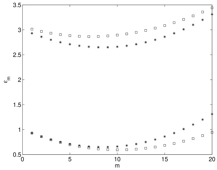
Figure 1: Energy levels in the two lowest Landau levels in an anharmonic trap with external rotation frequency $\Omega=1.1$ and anharmonicity $a=0.01$. Squares are the exact numerically computed energy levels. Asterisks denote the variational approximation using harmonic-oscillator eigenfunctions.

In order to make the problem tractable one needs to assume that no states are occupied except those in the lowest Landau level (LLL), i. e. the levels with no radial nodes, $n_{r}=0$. The restrictions on physical parameters needed for this assumption to hold will shortly be explored. In general, the single-particle spectrum in the LLL around the minimum can be approximated with a quadratic expression,

$$\epsilon_{\kappa}=\epsilon_{0}+\frac{\alpha}{2}{\kappa}^{2},$$ (4)

where $\kappa=m-m_{0}$ is a shifted azimuthal quantum number; the offset $m_{0}$ is the quantum number at which the energy has its minimum; and the curvature $\alpha$ has to, in general, be computed numerically. When the anharmonicity $a$ is very small, the energy spectrum can be solved perturbatively using harmonic-oscillator eigenfunctions, resulting in

$$\epsilon_{m}=\omega-(\Omega-1)m+\frac{a}{2}(m+1)(m+2).$$ (5)

Thus, in this limit the minimum-energy quantum number is given by

$$m_{0}=(\Omega-1)/a-3/2,$$ (6)

the curvature is $\alpha=a$, and the ground-state energy $\epsilon_{0}=1-m_{0}^{2}+a$. For not so small $a$, or high enough quantum numbers $m$, the corrections to the perturbative expressions become important, but they only result in quantitative shifts. In the following, we shall use the effective curvature parameter $\alpha$, which may be slightly different from $a$, in the calculations, but the more physical discussions and order-of-magnitude estimates will be stated in terms of the actual anharmonicity $a$.

The number of particles is determined by the chemical potential $\mu$, which in the weakly interacting limit is equal to the Fermi energy. For convenience, a Fermi quantum number $\kappa_{F}$ is defined through the relation

$$\mu=\epsilon_{0}+\frac{\alpha}{2}\kappa_{F}^{2},$$ (7)

so that the actual number of particles per spin state is $N=2\kappa_{F}$ in the weakly interacting limit, but one must bear in mind that it may differ from that when interactions are finite. The parameters are assumed to be such that $\mu<0$, implying $m_{0}-\kappa_{F}>0$. That way, the occupied part of the spectrum is bounded from below at some finite angular momentum quantum number $m>0$, and one can treat the spectrum as if it is extended indefinitely in both the positive and negative $\kappa$-direction.

The coupling constant $g$ introduced in Eq. (1) is a pseudopotential whose relation to the actual scattering length $a_{s}$ is in general nontrivial sensarma2006 , but in the weak-coupling limit it reduces to the simple form $g=4\pi a_{s}$. The conventional dimensionless coupling parameter in the study of trapped Fermi gases is the product $\zeta=k_{F}a_{s}$, the Fermi wavenumber times the s-wave scattering length. In terms of our Fermi quantum number $\kappa_{F}$ and coupling constant $g$, we obtain $\zeta=\alpha^{1/2}\kappa_{F}g/4\pi$, and we shall confine the study to small values of $\zeta$, i. e. weak coupling, in order not to violate the conditions for the model to be valid. We now discuss the conditions for the LLL assumption to hold. Firstly, the next lowest Landau level, with $n_{r}=1$, must lie higher than the chemical potential. The spacing between the Landau levels is $2$ (in the present units where $\omega=1$), so the condition is $\mu<\epsilon_{0}+2$ or in terms of physical quantitites,

$$\frac{a}{2}\left(\frac{N}{2}\right)^{2}<2.$$ (8)

Furthermore the condition $\mu<0$ stated above needs to be improved. Interactions broaden the occupation of fermions and smear out the Fermi level on a scale $|g|$, the interaction strength. The distance between the lower Fermi level and the edge of the spectrum at $m=0$ thus needs to be larger than $|g|$, that is, $m_{0}-\kappa_{F}>|g|$ or

$$\frac{\Omega-1}{a}-\frac{N}{2}>|g|.$$ (9)

Note that according to the first inequality, Eq. (8), $a$ must be of order $N^{-2}$ or smaller which means that the second restriction (9) is automatically fulfilled as long as $\Omega-1$ is positive and not smaller than $|g|N^{-2}$, which is an extremely small quantity. The first inequality does, however, put quite severe limitations on the experimental implementation of the state, since it forces the anharmonicity to be less than or of the order of the inverse square of the number of particles. These matters will be discussed further in the concluding section.

III Bogoliubov-de Gennes analysis

Through a number of assumptions on the physical parameters we have arrived at a description of a Fermi gas with a quadratic single-particle spectrum. This is the textbook case, and in principle, one may simply apply the usual textbook BCS expressions known for superconductors ll . Two things remain to be sorted out: first, the gap must be assumed to be larger than the level spacing, which permits us to treat the levels as a continuum (for paired Fermi systems with a discrete spectrum, see Ref. delft ). Second, one must consider the variation of the coupling with quantum number $\kappa$. This will have an effect on the density profile and quasi-particle energy spectrum, as we shall see.

The Bogoliubov-de Gennes (BdG) equation in two dimensions reads

$$\left(\begin{array}[]{ll}H_{0}-\mu&\Delta(r,\theta)\\ \Delta(r,\theta)^{*}&-H_{0}^{*}+\mu\end{array}\right)\left(\begin{array}[]{l}u_{\kappa}(r,\theta)\\ v_{\kappa}(r,\theta)\end{array}\right)=E_{\kappa}\left(\begin{array}[]{l}u_{\kappa}(r,\theta)\\ v_{\kappa}(r,\theta)\end{array}\right),$$ (10)

where we have anticipated that the solutions $u_{\kappa},v_{\kappa}$ can be labeled by the shifted angular momentum quantum number ${\kappa}$. When the single-particle energy spectrum is symmetric around $m=m_{0}$ (or ${\kappa}=0$), the gap function can be written

$$\Delta(r,\theta)=\Delta(r)e^{-i2m_{0}\theta}.$$ (11)

This amounts to assuming a cylindrically symmetric gap function and corresponds to the usual assumption of a homogeneous gap function in an infinite system. In order to match the $\theta$ dependence, the amplitudes take on the form

$$u_{\kappa}(r)=u_{\kappa}\phi_{m_{0}+{\kappa}}(r),$$

$$v_{\kappa}(r)=v_{\kappa}\phi_{m_{0}-{\kappa}}^{*}(r),$$ (12)

where $\phi_{m}$ are single-particle eigenfunctions in the anharmonic trap and $u_{\kappa}$ and $v_{\kappa}$ are space-independent amplitudes. The BdG equation (10) is now multiplied through by eigenfunctions $\phi_{m}$ and integrated, resulting in

$$\left(\begin{array}[]{cc}\xi_{\kappa}&\Delta_{\kappa}\\ \Delta_{\kappa}^{*}&-\xi_{\kappa}\end{array}\right)\left(\begin{array}[]{l}u_{\kappa}\\ v_{\kappa}\end{array}\right)=E_{\kappa}\left(\begin{array}[]{l}u_{\kappa}\\ v_{\kappa}\end{array}\right),$$ (13)

where

$$\Delta_{\kappa}=\int dr2\pi r\Delta(r)\phi_{m_{0}+\kappa}^{*}(r)\phi_{m_{0}-\kappa}^{*}(r),$$ (14)

and

$$\xi_{\kappa}=\varepsilon_{\kappa}-\mu=\frac{\alpha}{2}({\kappa}^{2}-{\kappa}_{F}^{2}).$$ (15)

The solution for the energies and amplitudes is similar to the traditional BCS expressions:

$$E_{\kappa}=\sqrt{\xi_{\kappa}^{2}+|\Delta_{\kappa}|^{2}},$$

$$u_{\kappa}^{2}=\frac{1}{2}(1+\frac{\xi_{\kappa}}{E_{\kappa}}),v_{\kappa}^{2}=\frac{1}{2}(1-\frac{\xi_{\kappa}}{E_{\kappa}}).$$ (16)

Now turn to the self-consistency equation for the gap function,

$$\Delta(r)=|g|\sum_{\kappa}u_{\kappa}(r)v^{*}_{\kappa}(r).$$ (17)

Inserting the calculated Bogoliubov amplitudes into the self-consistency equation, one obtains

$$\Delta(r) = |g|\sum_{\kappa}\phi_{m_{0}+{\kappa}}(r)\phi_{m_{0}-{\kappa}}(r)\frac{|\Delta_{\kappa}|}{2E_{\kappa}}.$$ (18)

Multiply by $\phi_{m_{0}+\kappa^{\prime}}(r)\phi_{m_{0}-\kappa^{\prime}}(r)$, integrate and rename the subscripts. The result is

$$\Delta_{\kappa}=|g|\sum_{\kappa^{\prime}}\frac{|\Delta_{\kappa^{\prime}}|}{2E_{\kappa^{\prime}}}V_{\kappa,\kappa^{\prime}}$$ (19)

where the coupling matrix element was defined as

$$V_{\kappa,\kappa^{\prime}} = \langle m_{0}+\kappa,m_{0}-\kappa|m_{0}+\kappa^{\prime},m_{0}-\kappa^{\prime}\rangle{\rm,and}$$

$$\langle m,n|k,l\rangle = \int dr\phi_{m}^{*}\phi_{n}\phi_{k}\phi^{*}_{l}.$$ (20)

In order to be able to produce a definite expression, let us make use of the results for a harmonic trap. Since Eq. (8) confines the parameters to lie in the regime of a very weak anharmonicity, the anharmonic trap can at most bring in small quantitative corrections. The matrix element for the contact potential in the space of harmonic-oscillator eigenfunctions is kavoulakis2000

$$\langle m,n|k,l\rangle=\frac{1}{2\pi}\frac{[(|m|+|n|+|k|+|l|)/2]!}{2^{(|m|+|n|+|k|+|l|)/2}\sqrt{|m|!|n|!|k|!|l|!}}.$$ (21)

Note that the potential is separable:

$$V_{\kappa,\kappa^{\prime}}\equiv V_{\kappa}V_{{\kappa}^{\prime}},\,V_{\kappa}=\sqrt{\frac{(2m_{0})!}{2\pi 2^{2m_{0}}(m_{0}+\kappa)!(m_{0}-\kappa)!}},$$ (22)

and furthermore, the potential is in the limit of large $m_{0}$ approximated by

$$V_{\kappa}\approx\frac{1}{\sqrt{2\pi}(\pi m_{0})^{1/4}}e^{\frac{-\kappa^{2}}{2m_{0}}}.$$ (23)

A separable potential presents a considerable simplification. The solution for the gap is

$$\Delta_{\kappa}=\Delta V_{\kappa},$$ (24)

where the constant $\Delta$ is found by solving the self-consistency equation in its final form,

$$1=|g|\sum_{\kappa}\frac{V_{\kappa}^{2}}{\sqrt{\Delta^{2}V_{\kappa}^{2}+\xi_{\kappa}^{2}}}.$$ (25)

This sum has, in general, to be computed numerically. Nevertheless, there is plenty of information to be extracted from its qualitative form, as we shall explore in the next section.

IV Parameter regimes

Consider the self-consistency equation (25). If the coupling is weak, $\Delta$ is expected to be small as well. In this case the largest contribution to the self-consistency sum comes from the states close to the Fermi surface, and the usual textbook BCS solution is recovered ll ,

$$\Delta=\omega_{c}e^{-1/(N(0)V_{00}|g|)},$$ (26)

where $\omega_{c}$ is the cut-off frequency for the sum and $N(0)$ is the density of states at the Fermi level. However, that solution is only valid when the interaction strength at the Fermi surface is larger than the separation of the energy levels; if it is smaller, one cannot neglect discreteness effects delft . This criterion translates to $|g|e^{-\kappa_{F}^{2}/m_{0}}/\sqrt{\pi m_{0}}>\alpha\kappa_{F}.$ On the other hand, if $|g|$ is too large, pairing will happen away from the Fermi surface, and as will shortly be shown, this occurs when $|g|>\alpha\kappa_{F}^{2}$. Combining the two inequalities, one finds that a criterion for avoiding both discreteness and off-Fermi surface pairing is

$$\frac{\kappa_{F}}{\sqrt{\pi m_{0}}}>e^{\kappa_{F}^{2}/m_{0}},$$ (27)

which cannot be fulfilled for any value of $\kappa_{F}$. We conclude that the standard textbook solution is not applicable in the present system.

We now derive the criterion already used above, for states away from the Fermi surface to contribute to the self-consistency sum. When the sum is exhausted by terms far from the Fermi surface we can write

$$|g|\sum_{|\kappa|\ll\kappa_{F}}\frac{V_{\kappa}^{2}}{\sqrt{\Delta^{2}V_{\kappa}^{2}+\xi_{\kappa}^{2}}}=1.$$ (28)

Setting $\Delta=0$ yields an inequality,

$$|g|\sum_{|\kappa|\ll\kappa_{F}}\frac{V_{\kappa}}{|\xi_{\kappa}|}>1.$$ (29)

The sum is estimated by inserting the maximum value of the summand and multiplying it by the effective range of the potential $V_{\kappa}$,

$$|g|\sqrt{2m_{0}}\frac{V_{0}^{2}}{|\xi_{0}|}>1,$$ (30)

where $\sqrt{2m_{0}}$ is the width of the function $V_{\kappa}$ and $V_{0}^{2}=(4\pi^{3}m_{0})^{-1/2}$ is its value in the region where the summand is at its largest. The factors involving $m_{0}$ cancel out, so the critical coupling strength for an off-Fermi surface contribution reduces to

$$|g|>g_{c}\propto|\xi_{0}|\propto\alpha\kappa_{F}^{2}.$$ (31)

In Fig. 2, the numerically computed value of $\Delta$ is plotted in various slices of parameter space. It is seen how the $\Delta=0.01$ level curve can be reasonably well fitted to Eq. (31) in all three plots. Beyond this curve, the discreteness of the spectrum is expected to be important and the BCS solution cannot be trusted to be quantitatively correct.

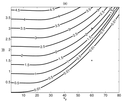
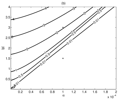
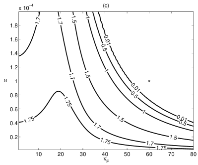
Figure 2: Level curves for the gap function $\Delta$ in three slices of parameter space. (a) Fixed anharmonicity $\alpha=0.0001$, (b) fixed Fermi quantum number $\kappa_{F}=60$, (c) fixed coupling $|g|=1.5$. The minimum-energy quantum number is fixed to $m_{0}=100$ in all three panels. Asterisks denote the phase-space points used in Fig. 3.

The quasi-particle spectrum differs qualitatively between the different parameter regimes. This is illustrated in Fig. 3.

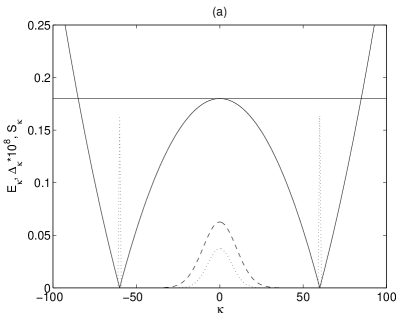
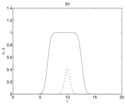
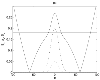
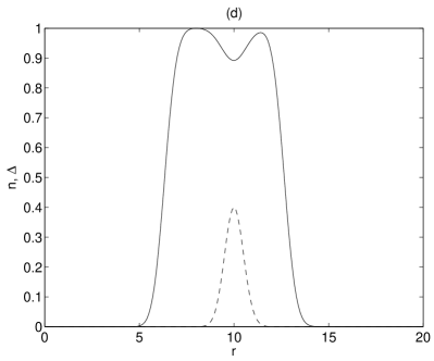
Figure 3: (a),(c): Full line: Quasi-particle energies $E_{\kappa}$. Dashed: $\kappa$-dependent gap function $\Delta_{\kappa}$. Dotted: summand $S_{\kappa}$ in the self-consistency sum. The gap function is magnified by a factor $10^{8}$ in (a). Horizontal line: chemical potential $\mu$. (b), (d): Spatial distributions of density (full line) and gap function $\Delta(r)$ (dashed). The gap function is scaled to have a peak value of 0.4. Parameters are chosen as $m_{0}=100$, $\kappa_{F}=60$, and $\alpha=0.0001$. (a-b): $|g|=0.3$, (c-d): $|g|=3.0$.

When $|g|\lesssim g_{c}$, one recognizes the textbook situation: pairing takes place mostly at the Fermi surface and the spectrum is equal to the absolute value of the single-particle spectrum except close to the Fermi surface, where a gap opens. On the scale of Fig. 3a, the gap is too small to be visible. The plot also includes the $\kappa$-dependent gap function $\Delta_{\kappa}$ and the summand in the self-consistency equation, Eq. (25), $S_{\kappa}=V_{\kappa}^{2}/E_{\kappa}$. It is seen that an appreciable contribution to the sum comes from terms close to the Fermi surface. If $|g|$ were even smaller, the sum would be entirely exhausted by the terms close to the Fermi surface, but as was found above, the BCS solution would be altered by effects associated with the discreteness of the spectrum. For stronger coupling, $|g|>g_{c}$, the pairing happens predominantly close to $\kappa=0$, where the interaction is at its maximum, as seen in Figs. 3c-d. The quasi-particle spectrum is affected in this region, but at larger $\kappa$ it resembles the usual BCS spectrum.

The spatial profile of the gap function is completely insensitive to the profile in $\kappa$-space of the summand as long as the population is confined to the LLL. It is given by the self-consistency equation in configuration space, Eq. (18),

$$\Delta(r)=|g|\sum_{\kappa}\phi_{m_{0}+{\kappa}}(r)\phi_{m_{0}-{\kappa}}(r)\frac{|\Delta_{\kappa}|}{2E_{\kappa}}=|g|\sum_{\kappa}\frac{|\Delta_{\kappa}|}{2E_{\kappa}}\frac{1}{\pi\sqrt{(m_{0}+{\kappa})!(m_{0}-{\kappa})!}}r^{2m_{0}}e^{-r^{2}/2}.$$ (32)

Thus, the gap function is a constant times the $2m_{0}$’th radial harmonic-oscillator eigenfunction. At the same time, the density is much broader as a function of $r$, and it does depend on the coupling. The density is

$$n(r)=2\sum_{\kappa}|\phi_{m_{0}-{\kappa}}(r)|^{2}|v_{\kappa}|^{2},$$ (33)

with $|v_{\kappa}|^{2}=(1-\xi_{\kappa}/E_{\kappa})/2$. It is a peculiar feature of the LLL states that each eigenfunction $\phi_{m_{0}-{\kappa}}(r)$ is confined to a very narrow, shell-like region in configuration space, centered at $r=(m_{0}-{\kappa})^{1/2}$. As a result, the distribution of particles in $\kappa$-space is mirrored by the spatial density profile, giving direct observational access to the distribution of particles in angular momentum space. For weak coupling, all states below the Fermi surface contribute, just as in ordinary BCS theory. The spatial profile as a function of the radial coordinate is a flattened, almost square profile, nicely mirroring the filled Fermi sea. As a result, only the interior of the toroidal density distribution is superfluid, while the outer regions are normal. For stronger coupling, the Bogoliubov amplitude $v_{\kappa}$ is depleted around $\kappa=0$ and the density profile has a dip in the region where the gap function is at its largest. Mathematically, it is easy to see why the density is depressed at the trap bottom when the coupling is strong: the Bogoliubov amplitude $v_{\kappa}$ is equal to half its peak value when $E_{\kappa}=\sqrt{\Delta_{\kappa}^{2}+\xi_{\kappa}}\gg\xi_{\kappa}$. Physically, it is the strong interactions that alter the occupation of the single-particle levels. As a result, one obtains a spatial region of strong Cooper pairing that shows up as a density depression. In the next section, we shall examine the conditions for this effect to persist when higher Landau levels are included.

V NLLL

In order to approach slightly more realistic territory in parameter space, let us now study what happens when the next lowest Landau level (NLLL) is brought into the calculation. Inspection of Eq. (8) reveals that this means allowing the product $aN^{2}/16$ to be slightly larger than unity. This system is still not easily realizable in experiment, but it is a first correction to the even more difficult LLL case studied above. The new Landau level introduces a new parameter into the system, namely, the energy difference between Landau levels, which is equal to $2\omega=2$ in dimensionless units. Thus, the balance between three main parameters determine the physics of the system as well as the validity of the truncation of the basis. The three are the chemical potential $\mu$, the coupling strength $g$, and the energy difference $2\omega$. In addition, the balance between the Fermi level $\kappa_{F}$ and the width of the coupling, $\sqrt{m_{0}}$, plays a role in determining the physics.

The single-particle eigenfunctions in the NLLL are

$$\phi_{m,1}(r)=\sqrt{\frac{m+1}{\pi m!}}\left(1-\frac{r^{2}}{m+1}\right)(re^{i\theta})^{m}e^{-r^{2}/2}.$$ (34)

The perturbative expression for the energies in the quartic trap are (see Fig. 1)

$$\epsilon_{m,1}=3\omega-(\Omega-\omega)m+\frac{a}{2}(m+2)(m+4).$$ (35)

The position of the energy minimum of the NLLL coincides with that of the LLL, $m_{0}$, to within $3/2$ quanta. That shift can safely be neglected here. On the other hand, when many Landau levels are brought into the calculation, the resulting asymmetry of the single-particle energy spectrum is likely to break the cylindrical symmetry such that the order parameter becomes a superposition of several angular-momentum states. The resulting profile is expected to be an annulus pierced by a ring of singly quantized vortices jackson2004 .

Now consider the coupling matrix elements. They are

$$V^{0001}_{\kappa,q} = \langle(m_{0}+\kappa,0),(m_{0}-\kappa,0)|(m_{0}+q,0),(m_{0}-q,1)\rangle$$ (36)

$$= \frac{(2m_{0})!(1-2q)}{2\pi 2^{2m_{0}}\sqrt{(m_{0}+q+1)!(m_{0}-q+1)!(m_{0}+\kappa)!(m_{0}-\kappa)!}}$$

$$\approx \frac{q-1}{\pi^{3/2}m_{0}}e^{-(\kappa^{2}+q^{2})/(2m_{0})}+{\mathcal{O}}(m_{0}^{-2}),$$

$$V^{0011}_{\kappa,q} = \frac{1}{4\pi}\frac{(2m_{0})!(m_{0}+1-2q^{2})}{2^{2m_{0}}\sqrt{(m_{0}+q+1)!(m_{0}-q+1)!(m_{0}+\kappa)!(m_{0}-\kappa)!}},$$ (37)

$$\approx \frac{1-2q^{2}/m_{0}}{4\pi\sqrt{\pi m_{0}}}e^{-(\kappa^{2}+q^{2})/(2m_{0})},$$

$$V^{0101}_{\kappa,q} = \frac{(2m_{0})!(1+m_{0}-\kappa-q+4\kappa q)}{8\pi 2^{2m_{0}}\sqrt{(m_{0}+q)!(m_{0}-q+1)!(m_{0}+\kappa)!(m_{0}-\kappa+1)!}}$$ (38)

$$\approx \frac{1}{4\pi\sqrt{\pi m_{0}}}e^{-(\kappa^{2}+q^{2})/(2m_{0})}\left(1+\frac{4\kappa q-q-\kappa}{2m_{0}}\right),$$

$$V^{1101}_{\kappa,q} = \frac{(2m_{0})!(1+m_{0}-2q-2m_{0}q-2\kappa^{2}+4\kappa^{2}q)}{2\pi 2^{2m_{0}}\sqrt{(m_{0}+q)!(m_{0}-q+1)!(m_{0}+\kappa+1)!(m_{0}-\kappa+1)!}}$$ (39)

$$\approx \frac{1-2q}{2\pi^{3/2}m_{0}}e^{-(\kappa^{2}+q^{2})/(2m_{0})},$$

$$V^{1111}_{\kappa,q} = \frac{1}{8\pi}\frac{(2m_{0})![2+3m_{0}^{2}-2(\kappa^{2}+q^{2})+m_{0}(5-2(\kappa^{2}+q^{2}))+4\kappa^{2}q^{2}]}{2^{2m_{0}}\sqrt{(m_{0}+q+1)!(m_{0}-q+1)!(m_{0}+\kappa+1)!(m_{0}-\kappa+1)!}}$$ (40)

$$\approx \frac{3}{8\pi\sqrt{\pi m_{0}}}(1-\frac{1+2(\kappa^{2}+q^{2})}{3m_{0}})e^{-(\kappa^{2}+q^{2})/(2m_{0})}.$$

The other matrix elements can be obtained from these by a sign change, e. g. $V^{0010}_{\kappa,q}=V^{0001}_{\kappa,-q}$. It is seen that these new matrix elements are not separable in the way that simplified the calculations within the LLL. Moreover, the matrix elements $V^{0001}$ and $V^{1101}$ are smaller than the others by a factor $m_{0}^{1/2}$; however, that does not mean that the inter-level coupling cannot be neglected, since the matrix elements $V^{0011}$ and $V^{0101}$ are still as large as the intra-level matrix elements.

Employing the cylindrically symmetric assumption for $\Delta(r)$ (keeping in mind that this may change when more Landau levels are brought into the problem), the ansatz for the Bogoliubov amplitudes has to be labeled by an angular momentum quantum number $\kappa$ and a branch index $j=0,1$ (enumerating the two solutions that exist for every $\kappa$),

$$u_{\kappa j}(r)=u_{\kappa j0}\phi_{m_{0}+\kappa,0}(r)+u_{\kappa j1}\phi_{m_{0}+\kappa,1}(r),$$

$$v_{\kappa j}(r)=v_{\kappa j0}\phi_{m_{0}-\kappa,0}^{*}(r)+v_{\kappa j1}\phi^{*}_{m_{0}-\kappa,1}(r).$$ (41)

The Bogoliubov equation for the $(k,j)$’th mode is

$$\left(\begin{array}[]{llll}\xi_{\kappa 0}&0&\Delta_{\kappa}^{00}&\Delta_{\kappa}^{01}\\ 0&\xi_{\kappa 1}&\Delta_{\kappa}^{10}&\Delta_{\kappa}^{11}\\ {\Delta_{\kappa}^{00}}^{*}&{\Delta_{\kappa}^{10}}^{*}&-\xi_{{\kappa}0}&0\\ {\Delta_{\kappa}^{01}}^{*}&{\Delta_{\kappa}^{11}}^{*}&0&-\xi_{{\kappa}1}\end{array}\right)\left(\begin{array}[]{l}u_{{\kappa}j0}\\ u_{{\kappa}j1}\\ v_{{\kappa}j0}\\ v_{{\kappa}j1}\end{array}\right)=E_{{\kappa}j}\left(\begin{array}[]{l}u_{{\kappa}j0}\\ u_{{\kappa}j1}\\ v_{{\kappa}j0}\\ v_{{\kappa}j1}\end{array}\right).$$ (42)

We have defined $\xi_{{\kappa}n}=\epsilon_{{\kappa}n}-\mu$ and the matrix elements

$$\Delta_{\kappa}^{nn^{\prime}}=\int d^{2}r\Delta(r)\phi_{m_{0}+{\kappa},n}^{*}\phi_{m_{0}-{\kappa},n^{\prime}}^{*}.$$ (43)

The self-consistency equation is in general

$$\Delta(r)=|g|\sum_{{\kappa}j}u_{{\kappa}j}(r)v_{{\kappa}j}(r)^{*},$$ (44)

and integrating one obtains

$$\Delta^{n_{1}n_{2}}_{\kappa}=|g|\sum_{{\kappa}^{\prime}j,n_{3},n_{4}}u_{j{\kappa}^{\prime}n_{3}}v^{*}_{j{\kappa}^{\prime}n_{4}}V^{n_{1}n_{2}n_{3}n_{4}}_{{\kappa}{\kappa}^{\prime}}.$$ (45)

The coupled equations are solved numerically. Figure 4 displays a few illustrative cases. It has been checked in trial calculations that the inclusion of more Landau levels does not alter the density profiles shown in this paper, and only marginally distorts the quasi-particle energy curves.

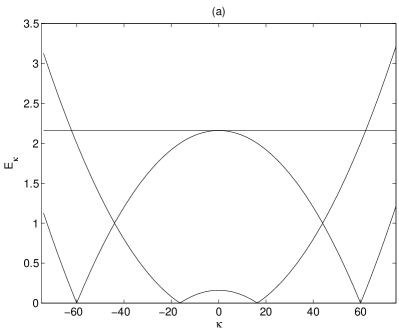
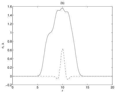
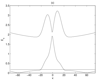
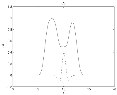
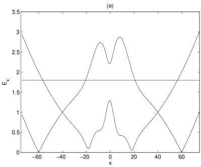
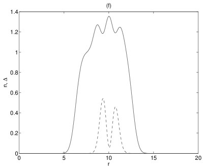
Figure 4: Energy spectra and density profiles calculated using two Landau levels (NLLL approximation). (a),(c),(e): Quasi-particle energies $E_{\kappa}$. Horizontal line: chemical potential $\mu$. (b), (d), (f): Spatial distributions of density (full line) and gap function $\Delta(r)$ (dashed). The gap function is scaled to have a peak value of 0.4 times the maximum density. Parameters are chosen as $m_{0}=100$, and ${\kappa}_{F}=60$. (a-b): $|g|=0.4$ and $\alpha=0.0012$, (c-d): $|g|=8.0$ and $\alpha=0.0001$, (e-f): $|g|=8.0$ and $\alpha=0.001$.

Basically, there are four parameter regimes of interest. When $\mu\ll 1$ and $|g|\ll 1$, the NLLL is not occupied at all. This case was studied in the previous section. When $\mu\sim 1$ and $|g|\ll 1$, the Fermi surface cuts through both energy bands, but the coupling is not too strong, as in Figs. 4a-b. There is a gap at the bottom of each of the two bands. The NLLL has a larger gap because the coupling is stronger for smaller ${\kappa}$. The associated density profile is expected to be bimodal, with an enhanced density in the interior of the toroidal cloud where two Landau levels are populated (cf. ho2000 ). Because the Fermi level has been limited to ${\kappa}_{F}=60$ in the numerical calculation, this “wedding cake” structure does not come out as clearly in Fig. 4b as it would in a bigger system. Figs. 4c-d illustrates the case where the chemical potential is small, but the coupling is comparable to the separation between the energy bands; $\mu\ll 1$ and $|g|\sim 1$. The Fermi level lies far below the NLLL, but because of the strong coupling, both levels are deformed. The resulting density profile is still depleted in the region of strong Cooper pairing, because the contribution from the NLLL is modest. For stronger interactions, more Landau levels are coupled and the NLLL approximation would fail. Note that the effect of the strong coupling on the quasi-particle spectrum is much more pronounced than the effect on the density. Finally, in Fig. 4e-f, both $\mu$ and $|g|$ are comparable to the inter-level gap. The energy levels are heavily distorted by the strong coupling. The density near $r=m_{0}^{1/2}$ is no longer depleted, because the NLLL states now occupy that regime. The gap function takes on a slightly nontrivial shape in configuration space; this is again an effect of the relatively few single-particle levels involved in the calculation. Trial calculations indicate that when the number of states is increased, the gap function acquires a smoother shape, but the contribution from the radially excited states broadens its profile compared to the LLL case.

Extrapolating from the results presented here, one may observe that the density is affected by two competing effects: as the Fermi surface includes more and more Landau levels, a “wedding cake” structure is expected in the density for weak interactions, but at the same time, strong interactions will deplete the interior of the toroidal density distribution.

VI Conclusion and outlook

This paper has shown that a Fermi superfluid trapped in an anharmonic potential can develop a giant vortex if it is rotated at high enough angular velocity, since the single-particle energy spectrum will then have its global minimum at a finite angular momentum. A giant-vortex state has been constructed in the basis of the lowest radially excited states, the lowest Landau level (LLL). Although attaining the LLL regime experimentally puts severe constraints on precision, the theoretical construction of such a state demonstrates that there exist parameter regimes in anharmonic traps for which a Fermi gas develops a giant vortex. As long as only the LLL is occupied, the density and gap function are cylindrically symmetric and form a toroidal profile. The superfluid region is confined to the interior of the torus, while the edges are normal. Since Cooper pairing is strongest in the center of the toroidal profile, the density is depleted in that region. The effect on the density appears, however, to be exclusive to the LLL. As more Landau levels are occupied, singly quantized vortices may form within the torus.

In order to have only the lowest Landau level populated in the quadratic plus quartic trap, the anharmonicity and rotation frequency have to be extremely fine tuned. In addition, any mechanical stirring method madison2000 will bring in corrections to the anharmonic trap that may be hard to control. It is therefore probably better to control the angular momentum of the gas by first stirring it in a harmonic potential and subsequently applying the anharmonicity. As an alternative to an extremely small quartic trapping term, an optical hard-wall potential at a suitably large distance from the trap center may be a more practical choice. It is possible that such a setup, with extensive amounts of fine tuning, may be a more practical route towards accessing the lowest Landau level.

Nevertheless, this study should first and foremost be seen as a demonstration by construction that trapped Fermi superfluids can sustain giant vortices. Several important issues remain to be studied, notably the size and shape of the allowed parameter regime for giant vortices; the physics in the BEC-BCS crossover regime; and whether giant vortices can ever be the favorable rotational configuration in purely harmonic traps. We hope to address these issues in future work.

- (1) E. M. Lifshitz and L. P. Pitaevskii, Statistical Physics Part 2 (Pergamon Press, Oxford, 1980).
- (2) C. J. Pethick and H. Smith, Bose-Einstein Condensation in Dilute Gases (Cambridge University Press, Cambridge, 2001).
- (3) K. W. Madison, F. Chevy, W. Wohlleben, and J. Dalibard, Phys. Rev. Lett. 84, 806 (2000).
- (4) C. Raman, J. R. Abo-Shaeer, J. M. Vogels, K. Xu, and W. Ketterle, Phys. Rev. Lett. 87, 210402 (2001).
- (5) M. W. Zwierlein, J. R. Abo-Shaeer, A. Schirotzek, C. H. Schunck, and W. Ketterle, Nature 435, 1047 (2005).
- (6) P. Singha Deo, V. A. Schweigert, and F. M. Peeters, Phys. Rev. Lett. 79, 4653 (1997).
- (7) D. A. Butts and D. S. Rokhsar, Nature 397, 327 (1999).
- (8) G. M. Kavoulakis, B. Mottelson, and C. J. Pethick, Phys. Rev. A 62, 063605 (2000).
- (9) Emil Lundh, Phys. Rev. A 65, 043604 (2002).
- (10) K. Kasamatsu, M. Tsubota, and M. Ueda, Phys. Rev. A 66, 053606 (2002).
- (11) Uwe R. Fischer and Gordon Baym, Phys. Rev. Lett. 90, 140402 (2003).
- (12) G. M. Kavoulakis and G. Baym, New J. Phys. 5, 51 (2003).
- (13) A. Aftalion and I. Danaila, Phys. Rev. A 69, 033608 (2004).
- (14) A. D. Jackson, G. M. Kavoulakis, and E. Lundh, Phys. Rev. A 69, 053619 (2004).
- (15) A. L. Fetter, B. Jackson, and S. Stringari, Phys. Rev. A 71, 013605 (2005).
- (16) H. Fu and E. Zaremba, Phys. Rev. A 73, 013614 (2006).
- (17) S. Bargi, G. M. Kavoulakis, and S. M. Reimann, Phys. Rev. A 73, 033613 (2006).
- (18) E. Lundh and H. M. Nilsen, e-print cond-mat/0608532 (2006).
- (19) M. Toreblad, M. Borgh, M. Koskinen, M. Manninen, and S. M. Reimann, Phys. Rev. Lett. 93, 090407 (2004).
- (20) R. Sensarma, M. Randeria, and T.-L. Ho, Phys. Rev. Lett. 96, 090403 (2006).
- (21) F. Braun and J. von Delft, Phys. Rev. Lett. 81, 4712 (1998).
- (22) T.-L. Ho and C. V. Ciobanu, Phys. Rev. Lett. 85, 4648 (2000).