Multiple time-scale approach for a system of Brownian particles in a non-uniform temperature field.

Abstract

The Smoluchowsky equation for a system of interacting Brownian particles in a temperature gradient is derived from the Kramers equation by means of a multiple time-scale method. The interparticle interactions are assumed to be represented by a mean-field description. We present numerical results that compare well with the theoretical prediction together with an extensive discussion on the prescription of the Langevin equation in overdamped systems.

I Introduction

The erratic motion of tiny particles suspended in a fluid of lighter particles is a known phenomenon, going under the name of Brownian motion, of fundamental interest in Statistical Mechanics Gardiner ; Risken ; Vankampen . A classical method to study this physical process is the Langevin equation, where the influence of the solvent particles on the heavier particles is modeled by two force terms. One term represents a viscous force, with friction coefficient $\gamma$, the other a stochastic force, whose intensity depends on the temperature of the solvent. Alternatively, the description of the dynamics of a system of Brownian particles in an external field may rest upon the Fokker-Planck equation (FPE) for the probability density of the particles. The two levels of description, namely, a) the Klein-Kramers equation Kramers , which considers the evolution of the probability density of position and velocity, and b) the Smoluchowski equation Smoluchowski , for the probability distribution of position only, have deserved a great deal of attention. The passage from the first description to the second one is well understood for the case of ideal non-interacting particles immersed in a heat bath at constant temperature. In fact, as shown by Wilemski and Titulaer Titulaer , the derivation of the Smoluchowski equation from the Kramers-Klein equation, can be performed by means of a perturbation expansion in terms of the inverse of the friction coefficient, $\gamma$. On the other side, one can derive the Smoluchowski equation more directly after taking the overdamped limit $\gamma\to\infty$ in the Langevin equation and neglecting the inertial acceleration term. Physically speaking, this procedure corresponds to the fact that the velocities of the particles thermalize rapidly, so that only the probability distribution of positions of the particles matters.

Thermal gradients, besides causing a heat flow, can induce a mass flow in systems such as colloids. The phenomenon is termed thermodiffusion, thermophoresis or Ludwig-Soret effect Ludwig ; Soret ; Landau ; Degroot ; Dhont ; Parola ; Bringuier and is relevant because it represents a tool to manipulate and concentrate molecules in solution. Thermophoresis, in fact, typically enhances the concentration in colder regions. Recently, it has been employed to form two dimensional colloidal crystals using $2\mu m$ polystyrene beads. Such a method leads to applications in microfiltration, particle accumulation and molecular detection on surfaces Duhr . Nevertheless, in spite of its technological interest, not many studies provide a derivation of the governing equation for the concentration field in the presence of a temperature gradient externally imposed. A problem arises when one considers the $\gamma\to\infty$ limit: the resulting stochastic equation contains a multiplicative noise term (the temperature is space-dependent). This in turn means that the associated FPE depends on the particular prescription used to derive it, i.e. one encounters the so called Ito-Stratonovich dilemma. To solve it, Matsuo and Sasa Sasa recently obtained the Smoluchowski equation from a perturbation expansion in powers of the inverse of $\gamma$. Two important messages arise from their work: first, the underdamped dynamics is free from the Ito-Stratonovich dilemma, and, second, their perturbation scheme is unbounded in time and one needs a renormalization treatment to make it convergent.

The main objective of this work is to present a systematic and convergent derivation of the Smoluchowski equation for a system of interacting Brownian particles in a temperature gradient. The interaction is of mean-field type, so that our starting point, the Kramers equation, can be written down in close form for the one-particle distribution function. We employ a multiple time-scale method which has been designed to deal with non-uniformities in systems with more than a time scale. The approach is quite appropriate for our objectives, since in the large friction limit there is a very clear time-scale separation in the system: in a very short period the velocities of the particles relax to their thermal equilibrium value, whereas on a much longer time scale also the positions of the particles assume configurations compatible with their steady state distribution. In this regard, the multiple time-scale method has been used to perform the passage from the Kramers to the Smoluchowski equation for an ideal gas at constant temperature as an expansion in powers of the small parameter $\gamma^{-1}$, providing a uniformly valid result Bocquet1 ; Bocquet2 . More recently, the case of interacting hard-core particles in isothermal systems has also been studied within this framework Umberto .

Another important part of this work is the discussion about the Ito versus Stratonovich description of the system. This is based on numerical results of the Langevin dynamics.

The plan of this paper is the following: in section II we present the full Langevin equation, its overdamped limit, and the corresponding Kramers and Smoluchowski descriptions of the system. In section III the derivation of the Smoluchowski equation with the multiple time-scale method is presented. In section IV we present the numerical results, with some discussion on the different Ito-Stratonovich prescriptions, and in section V we give our conclusions.

II Microscopic model. Smoluchowski and Kramers equations.

Let us consider a system of $N$ interacting Brownian particles of mass $m$ in an external force field. For the sake of simplicity, let us assume only one spatial dimension. The system is also under the influence of an external non-uniform temperature field so that the dynamics of the particles is given by:

$$\frac{dx_{i}}{dt} =v_{i},$$ (1)

$$m\frac{dv_{i}}{dt} =-m\gamma v_{i}+f_{ext}(x_{i})+\sum_{j\neq i}f_{int}(x_{i}-x_{j})+\sqrt{T(x_{i})}\xi_{i}(t),$$

for $i=1,...,N$, and where $\gamma$ is the friction coefficient, $T$ is a non-uniform heat-bath temperature, $f_{ext}$ is an external force, $f_{int}$ is the interaction force between pair of particles, and $\xi_{i}(t)$ is a Gaussian white noise with zero average and correlation

$$\langle\xi_{i}(t)\xi_{j}(s)\rangle=2\gamma mk_{B}\delta_{ij}\delta(t-s).$$ (2)

$\langle\cdot\rangle$ indicates the average over a statistical ensemble of realizations, and $k_{B}$ is the Boltzmann constant. To study the dynamics of the system we consider the single particle probability distribution function, $P(x_{i},v_{i},t)$, of the position and velocity variables. Its evolution is given by the Fokker-Planck equation Gardiner also known as Kramers equation:

$$\frac{\partial}{\partial t}P(x,v,t)+\Bigr{[}v\partial_{x}+\frac{f_{ext}(x)+f_{m}(x)}{m}\partial_{v}\Bigr{]}P(x,v,t)=\gamma\partial_{v}\Bigr{[}vP(x,v,t)+\frac{k_{B}T(x)}{m}\partial_{v}P(x,v,t)\Bigr{]}.$$ (3)

Here $f_{m}(x)$ is the molecular field which takes the form

$$f_{m}(x)=\int dx^{\prime}f_{int}(|x-x^{\prime}|)\rho(x^{\prime})=-\int dx^{\prime}\frac{dU(|x-x^{\prime}|)}{dx^{\prime}}\rho(x^{\prime}),$$ (4)

being $U(|x-x^{\prime}|)$ the pair potential energy (i.e. $f_{int}(x_{i}-x_{j})=\frac{\partial U(x_{i}-x_{j})}{\partial x_{i}}$), and $\rho(x)=\int dvP(x,v,t)$. It is very important to realize under what conditions on the interparticle interactions one can write down eq. (3) (see Umberto ). Note that with no approximations the Kramers-FPE for interacting particles for the one-particle distribution function, $P(x,v,t)$, depends on the two-particle distribution $P_{2}(x,v,x^{\prime},v^{\prime},t)$. The main hypothesis done in Eq. (3) is that whenever $U(x-x^{\prime})$ is a smooth function of particle separation one may assume a mean-field approximation for the two-particle distribution function $P_{2}(x,v,x^{\prime},v^{\prime},t)\approx P(x,v,t)P(x^{\prime},v^{\prime},t)$. In the following we shall define $f=f_{ext}+f_{m}$.

Since the temperature $T(x)$ in Eq. (3) multiplies a derivative with respect to $v$, one realizes that the Kramers equation is free from the so called Ito-Stratonovich dilemma. On the contrary, when one considers the overdamped limit, $\gamma\to\infty$, in Eq. (1) one obtains the following Langevin equation:

$$\frac{dx_{i}}{dt}=\frac{f(x_{i})}{m\gamma}+\frac{\sqrt{T(x_{i})}}{m\gamma}\xi_{i}(t),$$ (5)

which leads to different equations for the distribution of the spatial position (the so-called Smoluchowski equation) depending on the prescription adopted to integrate the stochastic evolution. In fact, the corresponding FPE for Ito and Stratonovich conventions, the two rules usually applied, are respectively:

$$\frac{\partial}{\partial t}P(x,t)=-\frac{1}{m\gamma}\partial_{x}(fP)+\frac{k_{B}}{\sqrt{m}\gamma}\partial_{x}^{2}(TP),$$ (6)

$$\frac{\partial}{\partial t}P(x,t)=-\frac{1}{m\gamma}\partial_{x}(fP)+\frac{k_{B}}{\sqrt{m}\gamma}\partial_{x}(T^{1/2}\partial_{x}(T^{1/2}P)).$$ (7)

The aim of this work is to derive a Smoluchowski equation for the system using the multiple time-scale method, via an expansion in the inverse of the friction coefficient. Our starting point is the Kramers equation, Eq. (3). At this stage it is convenient to introduce the following dimensionless variables:

$$\tau\equiv t\frac{v_{T}}{{\it l}},\qquad V\equiv\frac{v}{v_{T}},\qquad X\equiv\frac{x}{{\it l}},\qquad\Gamma=\gamma\frac{{\it l}}{v_{T}},$$ (8)

$$F(X)\equiv\frac{{\it l}f(x)}{mv_{T}^{2}},\qquad\tilde{P}(X,V,\tau)\equiv{\it l}v_{T}P(x,v,t),$$ (9)

being $v_{T_{0}}=\sqrt{k_{B}T_{0}/m}$ the thermal velocity at the reference temperature $T_{0}$ (which can be taken equal to $1$), and ${\it l}$ is a typical length scale of the system, for example the effective radius of the particles. The non-dimensional Kramers equation for $\tilde{P}(X,V,\tau)$ denoting, $\tilde{T}(X)=T(x)$, is:

$$\frac{\partial\tilde{P}(X,V,\tau)}{\partial\tau}=\Gamma\partial_{V}(V\tilde{P})+\Gamma\tilde{T}(X)\partial_{V}^{2}\tilde{P}-V\partial_{X}\tilde{P}-F\partial_{V}\tilde{P}.$$ (10)

In the following we shall skip the tildes in our notation. The (non-dimensional) Kramers equation, Eq. (10), is our definitive starting point and in the next section we proceed to present the set of eigenfunctions that will be used in the subsequent section when we make use of the multiple time-scale approach.

III Method of solution

Standard solutions of Eq. (10) go through an expansion in a basis set of eigenfunctions. First, it is convenient to separate the spatial dependence from the velocity dependence of the probability distribution. We rewrite Eq. (10) as:

$$\Gamma L_{FP}P(X,V,\tau)=\Bigr{[}\frac{\partial}{\partial\tau}+V\frac{\partial}{\partial X}+F\frac{\partial}{\partial V}\Bigr{]}P(X,V,\tau),$$ (11)

where we introduced the Fokker-Planck operator

$$L_{FP}P(X,V,\tau)=\frac{\partial}{\partial V}\Bigl{[}T(X)\frac{\partial}{\partial V}+V\Bigl{]}P(X,V,\tau).$$ (12)

We will expand $P$ in terms of the eigenfunctions $H_{\nu}(X,V)$ of $L_{FP}$ Sasa which are related to the Hermite polynomials:

$$L_{FP}H_{\nu}(X,V)=-\nu H_{\nu}(X,V)$$ (13)

with

$$H_{\nu}(X,V)\equiv\frac{T(X)^{\nu/2}}{\sqrt{2\pi T(X)}}(-1)^{\nu}\frac{\partial^{\nu}}{\partial V^{\nu}}\exp(-\frac{V^{2}}{2T(X)}).$$ (14)

We now express the solutions to Eq. (11) as a linear combination of products of the type $\phi_{\nu}(X,\tau)H_{\nu}(X,V)$ and after some algebra obtain:

$$\sum_{\nu=0}^{\infty}\Bigl{\{}\Bigl{[} \frac{\partial\phi_{\nu}(X,\tau)}{\partial\tau}+\Gamma\nu\phi_{\nu}(X,\tau)\Big{]}H_{\nu}(X,V)+$$

$$\sqrt{T(X)}\Bigl{[}\frac{\partial\phi_{\nu}(X,\tau)}{\partial X}-\frac{F(X)}{T(X)}\phi_{\nu}(X,\tau)\Bigl{]}H_{\nu+1}(X,V)+\sqrt{T(X)}\nu\frac{\partial\phi_{\nu}(X,\tau)}{\partial X}(\delta_{\nu,0}-1)H_{\nu-1}(X,V)$$

$$+\frac{T^{\prime}(X)}{2\sqrt{T(X)}}\phi_{\nu}(X,\tau)[H_{\nu+3}(X,V)+2(\nu+1)H_{\nu+1}(X,V)+\nu H_{\nu-1}(X,V)]\Bigl{\}}=0$$

where the prime denotes derivation with respect to the argument. Equating the coefficients of the same basis functions, $H_{\nu}$, we obtain an infinite hierarchy of equations relating the various moments $\phi_{\nu}(X,\tau)$. Such a hierarchy can be truncated by the multiple scale method, as shown hereafter.

III.1 Multiple time-scale analysis

In the multiple time-scale analysis one determines the temporal evolution of the distribution function $P(X,V,\tau)$ in the regime $\Gamma^{-1}<<1$ by means of a perturbative method.

In order to construct the solution one replaces the single physical time scale, $\tau$, by a series of auxiliary time scales ($\tau_{0},\tau_{1},..,\tau_{n}$) which are related to the original variable by the relations $\tau_{n}=\Gamma^{-n}\tau$. Also the original time-dependent function, $P(X,V,\tau)$, is replaced by an auxiliary function, $P_{a}(X,V,\tau_{0},\tau_{1},..)$, depending on the $\tau_{n}$, which are treated as independent variables. Once the equations corresponding to the various orders have been determined, one returns to the original time variable and to the original distribution.

We begin by replacing the time derivative with respect to $\tau$ by a sum of partial derivatives:

$$\frac{\partial}{\partial\tau}=\frac{\partial}{\partial\tau_{0}}+\frac{1}{\Gamma}\frac{\partial}{\partial\tau_{1}}+\frac{1}{\Gamma^{2}}\frac{\partial}{\partial\tau_{2}}+...$$ (16)

The auxiliary function, $P_{a}(X,V,\tau_{0},\tau_{1},...)$, is expanded as a series of powers of $\Gamma^{-1}$

$$P_{a}(X,V,\tau_{0},\tau_{1},\tau_{2},...)=\sum_{s=0}^{\infty}\frac{1}{\Gamma^{s}}P_{a}^{(s)}(X,V,\tau_{0},\tau_{1},\tau_{2},...).$$ (17)

Each term $P_{a}^{(s)}$ is then projected over the eigenfunctions $H_{\nu}$,

$$P^{(s)}_{a}(X,V,\tau_{0},\tau_{1},...)=\sum_{\nu=0}^{\infty}\psi^{(s)}_{\nu}(X,\tau_{0},\tau_{1},\tau_{2},...)H_{\nu}(X,V).$$ (18)

At this stage one substitutes the time derivative (16) and expressions (17)-(18) into Eq. (10), and identifying terms of the same order in $\Gamma^{-1}$ in the equations one obtains a hierarchy of relations between the amplitudes $\psi^{(s)}_{\nu}$. The advantage of the method over the naive perturbation theory is that secular divergences can be eliminated at each order of perturbation theory and thus uniform convergence is achieved.

The most important function in all this expansion is $\psi^{(0)}_{0}$. Its physical meaning becomes clear if one integrates over $V$ the auxiliary density probability function $P_{a}(X,V,\tau_{0},\tau_{1},\tau_{2},...)$. Assuming, as in the standard expansion, that $\psi^{(\nu)}_{0}=0$ for $\nu\geq 1$ one sees that $\psi^{(0)}_{0}$ is the spatial density probability function. We shall consider the partial derivative, $\partial_{\tau_{i}}\psi^{(0)}_{0}$, and obtain the evolution equation for $\psi^{(0)}_{0}$ to order $\Gamma^{-i}$. For the sake of completeness we briefly show how the method works. To order $\Gamma^{0}$ one finds:

$$L_{FP}\Bigr{[}\sum_{\nu}\psi^{(0)}_{\nu}H_{\nu}\Bigr{]}=0,$$ (19)

and concludes that only the amplitude $\psi^{(0)}_{0}$ is non-zero.

We consider, next, terms of order $\Gamma^{-1}$ and write (note that on the l.h.s we always have the application of the Fokker-Planck operator to the auxiliary function to the order of interest, in this case $s=1$) :

$$-(\psi^{(1)}_{1}H_{1}+2\psi^{(1)}_{2}H_{2}+3\psi^{(1)}_{3}H_{3}+\sum_{\nu\geq 3}\nu\psi^{(1)}_{\nu}H_{\nu})=H_{0}\partial_{\tau_{0}}\psi^{(0)}_{0}$$ (20)

$$+\sqrt{T(x)}H_{1}[\partial_{X}\psi^{(0)}_{0}-\frac{F}{T}\psi^{(0)}_{0}+\frac{T^{\prime}}{T}\psi^{(0)}_{0}]+\frac{T^{\prime}}{2\sqrt{T}}H_{3}\psi^{(0)}_{0}.$$

By equating the coefficients multiplying $H_{0}$ we find the relation:

$$\frac{\partial\psi^{(0)}_{0}}{\partial\tau_{0}}=0,$$ (21)

i.e. the amplitude $\psi^{(0)}_{0}$ is not a function of $\tau_{0}$. We also obtain for the amplitude $\psi^{(1)}_{1}$ the equations

$$\psi^{(1)}_{1}=\Bigl{[}-\sqrt{T(X)}\partial_{X}\psi^{(0)}_{0}+\frac{F}{\sqrt{T(X)}}\psi^{(0)}_{0}-\frac{T^{\prime}(X)}{\sqrt{T(X)}\psi^{(0)}_{0}}\Bigl{]}.$$ (22)

The remaining amplitudes are

$$\psi^{(1)}_{2}=0,\qquad\psi^{(1)}_{3}=-\frac{1}{6}\frac{T^{\prime}(X)}{\sqrt{T(X)}}\psi^{(0)}_{0},\qquad\psi^{(1)}_{\nu}=0\ \ if\ \ \ \nu\geq 3.$$ (23)

By iterating the method we obtain the correction of order $\Gamma^{-1}$ to the evolution equation of $\psi^{(0)}_{0}$, which reads

$$\partial_{\tau_{1}}\psi^{(0)}_{0}=-\partial_{X}(\sqrt{T}\psi^{(1)}_{1}),$$ (24)

and using Eq. (22) we can rewrite it as:

$$\partial_{\tau_{1}}\psi^{(0)}_{0}=\partial_{X}\Bigl{[}\partial_{X}(T\psi^{(0)}_{0})-F\psi^{(0)}_{0}\Bigl{]}$$ (25)

Finally, we recover the original time variable, $\tau$, and obtain the most important result of this work, that is, the evolution equation for the spatial probability density:

$$\partial_{\tau}\psi^{(0)}_{0}=\frac{1}{\Gamma}\partial_{X}\Bigl{[}\partial_{X}(T\psi^{(0)}_{0})-F\psi^{(0)}_{0}\Bigl{]}+O(1/\Gamma^{2}).$$ (26)

With $O(1/\Gamma^{2})$ we mean terms of or $1/\Gamma^{2}$ and superior. The first comment that arises from Eq. (26) is that it is of the Ito type if one uses this prescription for the overdamped Langevin equation. However, here we did not use any prescription for the Langevin equation, and Eq. (26) was derived from an expansion of the Kramers equation. Moreover, the generalization of Eq. (26) to arbitrary spatial dimensions is straightforward.

Using a more usual notation for the spatial density probability function, and following the line of reasoning of Marconi and Tarazona Tarazona , one could write the following governing equation

$$\frac{\partial\rho(x,t)}{\partial t}=\nabla\Bigr{\{}\nabla D(x)\rho(x,t)+\frac{1}{m\gamma}\rho(x,t)\nabla\bigr{[}\frac{\delta{\cal F}_{ni}[\rho]}{\delta\rho(x,t)}+V_{ext}(x)\bigr{]}\Bigr{\}},$$ (27)

where $D(x)=k_{B}T(x)/m\gamma$ and ${\cal F}_{ni}$ is the excess over the ideal gas contribution to the free energy Archer . The second term renormalizes the effective diffusion constant of the particles and may become important at higher concentrations.

In the next section we proceed to check numerically our results and to enter in a possible discussion about the Ito-Stratonovich dilemma.

IV Numerical results

This section is devoted to numerically check our analytical results. The way to proceed is to compare the results of numerical simulations of a system of $N$ particles following the dynamics given by Eqs. (1) or rather Eq. (5). We shall compare these with the analytical solution, if available, of the corresponding density equation: Eq. (26) for the first case, or the Smoluchowski in the Ito and Stratonovich prescriptions, Eqs. (6-7), for the second case.

In order to obtain a simple analytical solution of the density equation we assume a vanishing external force and molecular field, $F=0$, particles have mass one, the system is one-dimensional and particles positions restrict to the interval $[0,1]$. We also assume that the temperature field has a linear spatial dependence $T(X)=T_{0}+T_{1}X$, with $T_{0}$ and $T_{1}$ positive constants. Finally, we impose zero flux boundary conditions of the system at the extremes of the spatial interval, i.e., there are infinite walls at these extremes where the particles rebound and cannot scape from the system.

The equation for the probability density that we have derived from the Kramers equation with the multiscale approach in an expansion in $\Gamma$, Eq. (26), is now (for aesthetic reasons we denote in the following $\psi^{(0)}_{0}(X,\tau)=\rho(X,\tau)$)

$$\partial_{\tau}\rho(X,\tau)=\frac{1}{\Gamma}\partial^{2}_{X}(T(X)\rho)=-\partial_{X}J(X),$$ (28)

where $J$ is the flux. The boundary conditions read $J(0)=J(L)=0$. The stationary solution is given by:

$$\rho^{s}(X)=\frac{NT_{1}}{(T_{0}+T_{1}X)\ln{[(T_{0}+T_{1}L)/T_{0}]}},$$ (29)

where we have used the normalization condition $\int_{0}^{L}dX\rho^{s}(X)=N$.

On the other side, in the overdamped limit one has to distinguish between the two prescriptions. In this paper we discuss the two more standard: Ito and Stratonovich. The Ito-Smoluchowski equation is also given by Eq. (28) and the stationary solution is obviously given by Eq. (29). A very important difference here is that it has not been derived as an expansion of inverse powers of $\Gamma$, and thus it is exact and no higher order corrections should appear. In the Stratonovich prescription the density equation, which is also exact and not an approximation to order $\Gamma^{-1}$, is given by:

$$\partial_{\tau}\rho(X,\tau)=\frac{1}{\Gamma}\partial_{X}(T^{1/2}\partial_{X}T^{1/2}\rho).$$ (30)

With the same boundary conditions the stationary Stratonovich solution is given by:

$$\rho^{s}_{strat}=\frac{NT_{1}}{(T_{0}+T_{1}X)^{1/2}[2(\sqrt{T_{0}+T_{1}L}-\sqrt{T_{0}})]}$$ (31)

Now we show the numerical results for the Langevin particle dynamics. We begin with the underdamped dynamics, and consider $2000$ particles evolving according to Eq. (1). We take $T_{0}=0.1$ and $T_{1}=10$ and all our measurements are performed when the system is stationary. Average values are obtained by sampling $200$ different realizations. A stationary density of particles is defined at every spatial point by counting the number of particles in every cell of size $dx=1/1000$. The time step used is $dt=0.0001$. For different values of $\Gamma$ the results are shown in Fig. 1. One can see that for large values of $\Gamma$ the comparison with the analytical result, Eq. (29), is excellent. Obviously, the smaller the value of $\Gamma$ the larger the corrections that we are neglecting and the agreement worsens.

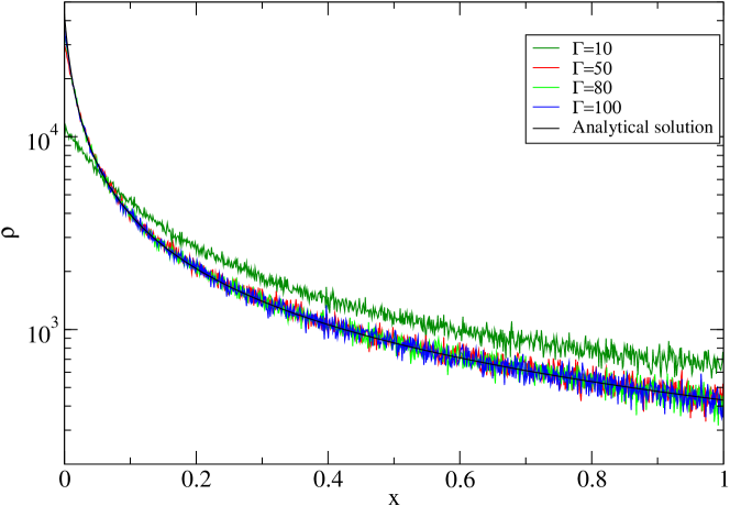
Figure 1: (color online) Plot of the stationary density of particles for different values of $\Gamma$. The particle dynamics correspond to the Langevin equation Eq. (1), and the density of particles has been computed by making a coarse-graining in the particle positions. With the solid black line we plot the analytical solution Eq. 29, that fits well for large $\Gamma$ values. The other parameters used in the simulation are $dt=0.0001$ and the cell size for the coarse-graining $dx=1/1000$.

In Fig. 2 we show the results obtained from the simulations of the overdamped dynamics, Eq. (5), where we have also coarse-grained the distribution of particles to compute a density of particles. Interpreting it like Ito the results are in perfect agreement with the Ito-Smoluchowski stationary solution, Eq.(29). This is shown in the left panel of the figure for different values of $\Gamma$. When it is understood in the Stratonovich calculus, for which we have to add a new term $\frac{T^{\prime}(X)}{2m\gamma}$ in the r.h.s. of Eq. (5) to make the numerical simulation, again the results coincide with the stationary density solution in the Stratonovich calculus, Eq. (31), as shown in the right panel of Fig. 2 for various values $\Gamma$. A very important difference encountered in these results with respect to those in Fig. 1 is their independence with respect to the value of $\Gamma$: for any of its values the agreement with the stationary density is always excellent. In fact, one can realize that once the limit has been performed, the value of $\Gamma$ only renormalises the time scale of the problem.

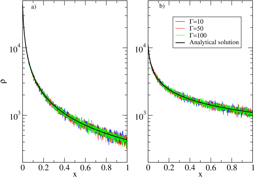
Figure 2: (color online) Coarse-grained density field obtained from the overdamped Langevin dynamics Eq. 5. Left panel corresponds to the Ito interpretation of this equation, and right to the Stratonovich one. We take different values of the parameter $\Gamma$ as indicated in the legend box. With the solid line we plot the stationary density solutions as given by Eqs. 29 and 30, for Ito and Stratonovich respectively. The rest of the parameters used in the simulation are $dt=0.0001$ and the cell size to make the coarse-graining of the position of the particles is $dx=1/1000$.

V Conclusions

In the present paper, we have derived the form of the governing equation for the probability density of interacting Brownian particles in the case of an inhomogeneous medium, whose temperature varies in space. The interparticle interactions have been treated in a mean-field framework. We have shown, using the Klein-Kramers equation associated to the fully inertial stochastic dynamics, that, to leading order, one obtains a Smoluchowski equation for the particle distribution which has the same form as the equation obtained by applying the Ito prescription to the overdamped dynamics.

VI Acknowledgments

C.L. acknowledges financial support from MEC (Spain) and FEDER through project CONOCE2 (FIS2004-00953) and from the bilateral project Spain-Italy HI2004-0144. He also acknowledges a Ramón y Cajal research fellow of the Spanish MEC. U.M.B.M. acknowledges a grant COFIN-MIUR 2005, 2005027808.

References

- (1) C. Gardiner, Handbook of Stochastic methods for Physics, Chemistry and in the Natural Sciences (Springer-Verlag, Berlin, 1994).
- (2) H. Risken, The Fokker-Planck Equation (Springer-Verlag, Berlin, 1984).
- (3) N. van Kampen, Stochastic Processes in Physics and Chemistry (North-Holland, Amsterdam, 1992).
- (4) H.A. Kramers, Physica A, 7, 284 (1940).
- (5) M. von Smoluchowski, Ann.Phys., 48, 1103 (1916).
- (6) G. Wilemski, J. Stat. Phys. 14, 153 (1976); U.M. Titulaer, Physica A 91, 321 (1978) and Physica A 100, 234 (1980).
- (7) C. Ludwig, Sitzber. Kaiserl. Akad. Wiss. Math.-Natwiss. Kl. (Wien) 20, 539 (1856).
- (8) C. Soret, Arch Sci. Phys. Nat. (Geneva) 2(3), 48 (1879).
- (9) L. Landau and E. Lifshitz, Fluid Mechanics (Mir, Moscow, 1951).
- (10) S. R. de Groot and P. Mazur, Non-equilibrium Thermodynamics (Dover, New York, 1984).
- (11) J.K.Dhont, J.Chem.Phys. 120, 1632 (2004).
- (12) A.Parola and R.Piazza, Eur.Phys.J. E 15, 255 (2004).
- (13) E. Bringuier and A. Bourdon Phys. Rev. E 67, 011404 (2003)
- (14) S.Duhr and D.Braun, Phys. Rev. Lett. 96, 168301 (2006).
- (15) M. Matsuo and S.-i. Sasa, Physica A 276, 188 (2000).
- (16) L. Bocquet, Am. J. Phys. 65, 140 (1997).
- (17) J. Piasecki, L. Bocquet and J.P. Hansen, Physica A 218, 125 (1995).
- (18) U. Marini Bettolo Marconi and P. Tarazona, J. Chem. Phys. 124, 164901 (2006).
- (19) U. Marini Bettolo Marconi and P.Tarazona, J. Chem. Phys. 110, 8032 (1999) and J.Phys.: Condens. Matter 12, 413 (2000).
- (20) A.J.Archer and R.Evans J. Chem. Phys. 121 4246 (2004).