Single-Particle Density of States of a Superconductor with a Spatially Varying Gap and Phase Fluctuations

Abstract

Recent experiments have shown that the superconducting energy gap in some cuprates is spatially inhomogeneous. Motivated by these experiments, and using exact diagonalization of a model $d$-wave Hamiltonian, combined with Monte Carlo simulations of a Ginzburg-Landau free energy functional, we have calculated the single-particle density of states LDOS$(\omega,r)$ of a model high-T_c superconductor as a function of temperature. Our calculations include both quenched disorder in the pairing potential and thermal fluctuations in both phase and amplitude of the superconducting gap. Most of our calculations assume two types of superconducting regions: $\alpha$, with a small gap and large superfluid density, and $\beta$, with the opposite. If the $\beta$ regions are randomly embedded in an $\alpha$ host, the LDOS on the $\alpha$ sites still has a sharp coherence peak at $T=0$, but the $\beta$ component does not, in agreement with experiment. An ordered arrangement of $\beta$ regions leads to oscillations in the LDOS as a function of energy. The model leads to a superconducting transition temperature $T_{c}$ well below the pseudogap temperature $T_{c0}$, and has a spatially varying gap at very low $T$, both consistent with experiments in underdoped Bi2212. Our calculated LDOS$(\omega,r)$ shows coherence peaks for $T<T_{c}$, which disappear for $T>T_{c}$, in agreement with previous work considering phase but not amplitude fluctuations in a homogeneous superconductor. Well above $T_{c}$, the gap in the LDOS disappears.

I Introduction

According to low temperature scanning tunneling microscopy (STM) experiments, the local density of states (LDOS) of some cuprate materials have spatial variations cren ; pan_davis ; howald1 ; lang_davis ; howald2 ; fang ; kato_sakata ; mashima . Among the cuprates, Bi₂Sr₂CaCu₂O_8+x (Bi2212) is one of the most extensively studied in STM experiments. The LDOS spectrum shows that some regions of that material, which we will call $\alpha$-regions, have a small energy gap with large and narrow coherence peaks (reminiscent of the spectra observed in bulk superconducting materials), while other regions, which we will call $\beta$-regions, have a larger gap, but smaller and broadened peaks (which are reminiscent of the spectra seen in bulk pseudogap phase of some materials . These inhomogeneities occur on length scales of order 30$\AA$. Because at low doping concentrations $\alpha$ regions with “good” superconductivity are immersed in more metallic or semiconducting $\beta$ regions, some workers have made an analogy between these materials and granular superconductors lang_davis ; joglekar : superconducting domains spatially separated from one another by non-superconducting regions, but connected through proximity effect or Josephson tunneling.

At present there is no general agreement regarding the origin of the inhomogeneities in the cuprate superconductors —whether they are in charge density, spin density, LDOS, or other properties scalapino_nunner_hirschfeld . One hypothesis is that these inhomogeneities originate in a process of self organization due to competing orders zaanen ; emery_lin ; emery_kivelson ; low_emery ; emery_kivelson_tranquada ; jamei ; valdez_stroud . In another approach, the spatially varying properties of the cuprates are attributed to crystal defects or impurities. In particular, it has been suggested that the inhomogeneities in the LDOS originate in the random spatial distribution of dopant atoms near the copper oxide (CuO₂) planes pan_davis ; martin_balatsky ; wang_pan ; atkinson ; nunner_andersen_hirscfeld .

Several workers have studied the LDOS of inhomogeneous superconductors at low $T$. For example, Ghosal et alghosal have calculated the LDOS of a strongly disordered $s$-wave superconducting layer in two dimensions, solving the Bogoliubov-de Gennes equations self-consistently. They have also done similar work on a model of $d$-wave superconductivityghosal1 . Fang et al.fang , using a Green’s function approach, computed the zero temperature LDOS of a model lattice Hamiltonian in which one small region of the lattice has an different (either suppressed or enhanced) pairing strength than the rest; they find good agreement with experiments. Cheng and Su cheng_su have also explored how the LDOS is affected by a single spatial inhomogeneity in the pairing strength of a BCS Hamiltonian; they find that an inhomogeneity with an LDOS most closely resembling the experimental results is produced by an inhomogeneity with a cone-shaped distribution of the pairing strength; this work thus suggests that it is the small-length-scale variation of the pairing strength that causes incoherence in the LDOS. Mayr et al. mayr_dagotto have studied a phenomenological model with quenched disorder and observed a pseudogap in the LDOS caused by a mixture of antiferromagnetism and superconductivity, while Jamei et al. jamei_kapitulnik_kivelson have investigated the low order moments of the LDOS and their relation to the local form of the Hamiltonian.

In this paper we propose a phenomenological approach to study the effect of inhomogeneities on the LDOS in a model for cuprate superconductors. The model is a mean-field BCS Hamiltonian with $d$-wave symmetry, in which the pairing-field is inhomogeneous and also undergoes thermal fluctuations in both phase and amplitude at finite temperatures $T$. It has been argued scalapino_nunner_hirschfeld that the superconducting state of optimally doped to overdoped cuprates is well described by the BCS theory which includes a $d$-wave gap and scattering from defects outside the Cu0₂ plane. Instead of including such defects explicitly in our BCS Hamiltonian, we implicitly include their possible effects through inhomogeneities of the pairing-field amplitude. Furthermore, instead of self-consistently solving the Bogoliubov-de Gennes equations resulting from this model, we obtain the magnitude and phase of the complex pairing-field from Monte Carlo simulations based on a Ginzburg Landau free energy functional. Thus the procedure is as follows. First, we set the parameters of the Ginzburg Landau free energy functional from experiments. Next, using Monte Carlo simulations of this free energy, we obtain the pairing-field amplitudes which we then include in the BCS Hamiltonian. Finally, we diagonalize the latter in order to obtain the LDOS.

Now in optimally or nearly optimally doped Bi2212, the layers consist of randomly distributed $\beta$-regions immersed in a majority background of $\alpha$-regions pan_davis . We therefore choose Ginzburg-Landau parameters so as to reproduce this morphology at $T=0$, then carry out simulations at both zero and finite $T$ to obtain the LDOS in the different spatial regions.

At $T=0$ we compare these simulation results to those obtained using ordered instead of random arrangements of inhomogeneities. We find that the LDOS of the random systems much more closely resemble experiment. Specifically, regions with a small gap have sharp coherence peaks, while large-gap regions show lower and broader peaks. By contrast, systems with ordered inhomogeneities have LDOS spectra with sharp coherence peaks which oscillate as a function of energy. In the ordered systems, the coherence peaks in the small-gap regions strongly resemble those observed in a homogeneous small-gap system. But the spectral peaks in the large-gap regions dramatically differ from those in the corresponding homogeneous and disordered cases.

Because the spectra of disordered systems more closely resemble experiments, we have also studied the evolution of the LDOS in these systems with increasing $T$. We consider both $T<T_{c}$ and $T>T_{c}$, where $T_{c}$ is the phase-ordering transition temperature (equivalent to the Kosterlitz-Thouless transition temperature for this two-dimensional system). In both the $\alpha$ and $\beta$ regions, we find that the spectral gap starts to fill in as $T$ increases, and the spectral peaks broaden and are reduced in height. However, even above $T_{c}$, the LDOS is still suppressed at low energies, in comparison to the normal state. This result agrees with a previous study eckl ; eckl2 which considered thermal fluctuations of the phase but not of the magnitude of the complex pairing-field, and included no quenched disorder.

We have also studied the $T$-dependence of the magnitude of the pairing field, its thermal fluctuations, and the effective superfluid density of our disordered system. We find that the phase ordering temperature is greatly reduced from the spatial average of the mean-field transition temperatures appearing in the Ginzburg Landau free energy functional. This reduction is due to both thermal fluctuations and quenched disorder in our model.

Although our work involves a non-self-consistent solution of a $d$-wave BCS Hamiltonian, it differs from previous studies of this kindfang ; ghosal ; ghosal1 ; cheng_su because it includes thermal fluctuations as well as quenched disorder in the pairing-field amplitude. For our model, quenched disorder is crucial in obtaining LDOS spectra which depend smoothly on energy and are also consistent with the observed low and broad peaks in the $\beta$ regions.

The rest of this article is organized as follows: In Section II, we present the BCS model Hamiltonian. In Section III, we derive the discrete form of the Ginzburg Landau free energy functional used in our calculations. We also discuss simple estimates of the phase ordering temperature, our choice of model parameters and our method of introducing inhomogeneities into our model. Section IV describe the computational methods used at both zero and finite temperature. These methods include a classical Monte Carlo approach to treat thermal fluctuations, exact diagonalization to obtain the LDOS, and the reduction of finite size effects on the LDOS by the inclusion of a magnetic field. Section V presents our numerical results at both $T=0$ and finite $T$. A concluding discussion and summary are given in Section VI.

II Model

II.1 Microscopic Hamiltonian

We consider the following Hamiltonian:

$$H_{BCS}=2\sum_{\langle i,j\rangle,\sigma}t_{ij}c_{i\sigma}^{\dagger}c_{j\sigma}+2\sum_{\langle i,j\rangle}(\Delta_{ij}c_{i\downarrow}c_{j\uparrow}+\text{c.c.})-\mu\sum_{i,\sigma}c_{i\sigma}^{\dagger}c_{i\sigma}$$ (1)

Here, $\sum_{\langle i,j\rangle}$ denotes a sum over distinct pairs of nearest neighbors on a square lattice with $N$ sites, $c_{j\sigma}^{\dagger}$ creates an electron with spin $\sigma$ ($\uparrow$ or $\downarrow$) at site $j$, $\mu$ is the chemical potential, $\Delta_{ij}$ denotes the strength of the pairing interaction between sites $i$ and $j$, and $t_{ij}$ is the hopping energy, which we write as

$$t_{ij}=-t_{hop}.$$ (2)

where $t_{hop}>0$.

Following a similar approach to that of Eckl et al. eckl , we take $\Delta_{ij}$ to be given by

$$\Delta_{ij}=\frac{1}{4}\frac{|\Delta_{i}|+|\Delta_{j}|}{2}e^{i\theta_{ij}},$$ (3)

where

$$\theta_{ij}=\begin{cases}(\theta_{i}+\theta_{j})/2,&\text{if bond $\langle i,j\rangle$ is in $x$-direction,}\\ (\theta_{i}+\theta_{j})/2+\pi,&\text{if bond $\langle i,j\rangle$ is in $y$-direction,}\end{cases}$$ (4)

and

$$\Delta_{j}=|\Delta_{j}|e^{i\theta_{j}},$$ (5)

is the value of the complex superconducting order parameter at site $j$. We will refer to the lattice over which the sums in (1) are carried out as the atomic lattice (in order to distinguish it from the XY lattice, which will be described in the next section.) The first term in Eq. (1) thus corresponds to the kinetic energy, the second term is a BCS type of pairing interaction with $d$-wave symmetry, and the third term is the energy associated with the chemical potential.

Eq. (1) may also be written

$$H_{BCS}=\Psi^{\dagger}\hat{A}\ \Psi-N\mu,$$ (6)

where

$$\Psi\equiv\left(\begin{array}[]{c}c_{i\uparrow}\\ c_{i\downarrow}^{\dagger}\end{array}\right),\quad\text{$i=1,N$}$$ (7)

and

$$\hat{A}=\left[\begin{array}[]{cc}\hat{t}&\hat{\Delta}^{\ast}\\ \hat{\Delta}&-\hat{t}^{\ast}\end{array}\right].$$ (8)

Here $\hat{t}$ and $\hat{\Delta}$ are $N\times N$ matrices with elements $\hat{t}_{ij}$ [$\hat{t}_{ij}=t_{ij}$, as given by eq. (2) if $i$ and $j$ are nearest-neighbors, $\hat{t}_{ij}=-\mu$ if $i=j$, and $\hat{t}_{ij}=0$ otherwise] and $\hat{\Delta}_{ij}$ [$\hat{\Delta}_{ij}=\Delta_{ij}$, as given by eq. (3) if $i$ and $j$ are nearest-neighbors, and $\hat{\Delta}_{ij}=0$ otherwise].

Let $\hat{U}$ be the unitary matrix that diagonalizes $\hat{A}$, i. e.,

$$\hat{B}=\hat{U}^{\dagger}\hat{A}\ \hat{U},\quad\quad\hat{B}\quad\text{diagonal.}$$ (9)

We can then rewrite (6) as

$$H_{BCS}=\Phi^{\dagger}\hat{B}\ \Phi-N\mu,$$ (10)

with $\Phi$ defined by

$$\Psi=\hat{U}\ \Phi.$$ (11)

If we make the following definitions:

$$\Phi\equiv\left(\begin{array}[]{c}\gamma_{i\uparrow}\\ \gamma_{i\downarrow}^{\dagger}\end{array}\right),\quad\text{$i=1,N$}$$ (12)

and

$$\hat{U}\equiv\left[\begin{array}[]{cc}u_{j}(r_{i})&-v_{j}^{\ast}(r_{i})\\ v_{j}(r_{i})&u_{j}^{\ast}(r_{i})\end{array}\right],\quad\text{$i$, $j=1,N$,}$$ (13)

where $i$ labels the row and $j$ the column of $N\times N$ matrices, then we can see that (11) is the typical Bogoliubov - de Gennes transformation tinkham ; degennes :

$$c_{i\uparrow}=\sum_{j=1}^{N}[\gamma_{j\uparrow}u_{j}(r_{i})-\gamma_{j\downarrow}^{\dagger}v_{j}^{\ast}(r_{i})],$$

$$c_{i\downarrow}=\sum_{j=1}^{N}[\gamma_{j\downarrow}u_{j}(r_{i})+\gamma_{j\uparrow}^{\dagger}v_{j}^{\ast}(r_{i})].$$ (14)

Thus $\Phi$ is a $2N$-dimensional column matrix and $\hat{U}$ is a $2N\times 2N$-dimensional square matrix.

Denoting the diagonal elements of the matrix $\hat{B}$ by $E_{n}$, we can use (8), (9) and (13) to obtain

$$\left[\begin{array}[]{cc}\hat{t}&\hat{\Delta}^{\ast}\\ \hat{\Delta}&-\hat{t}^{\ast}\end{array}\right]\left[\begin{array}[]{c}u_{n}(r_{i})\\ v_{n}(r_{i})\end{array}\right]=E_{n}\left[\begin{array}[]{c}u_{n}(r_{i})\\ v_{n}(r_{i})\end{array}\right].$$ (15)

Eq. (15) is the eigenvalue problem which must be solved in order to compute the local density of states, as we describe next.

II.2 Explicit expression for the local density of states

We wish to compute the local density of states, denoted LDOS$(\omega,r_{i})$, as a function of the energy $\omega$ and lattice position $r_{i}=(x_{i},y_{i})$ at both zero and finite temperature $T$. Given the value of the of the superconducting order parameter $\Delta_{i}$ at each lattice site, the matrix $\hat{\Delta}$ can be constructed and the $\text{LDOS}(\omega,r,\{\Delta_{i}\})$ can be computed through ghosal

$$\text{LDOS}(\omega,r_{i},\{\Delta_{i}\})=\sum_{n,E_{n}\geq 0}[|u_{n}(r_{i})|^{2}\delta(\omega-E_{n})+|v_{n}(r_{i})|^{2}\delta(\omega+E_{n})]$$ (16)

At $T=0$ all the phases $\theta_{i}$ are the same, since this choice minimizes the energy of the superconducting system. Thus, in this case, once we know $\{|\Delta_{i}|\}$ we can solve eq. (15) for $u_{n}(r_{i})$, $v_{n}(r_{i})$ and $E_{n}$, and use this solution in (16). At finite $T$, since $\Delta_{i}$ will thermally fluctuate, we need a procedure to obtain an average of (16) over the relevant configurations of $\{\Delta_{i}\}$. We explain that procedure next.

III Model for thermal fluctuations

At finite $T$ we compute LDOS$(\omega,r_{i})$ by performing an average of $\text{LDOS}(\omega,r_{i},\{\Delta_{i}\})$ over different configurations $\{\Delta_{i}\}$. Those configurations are obtained assuming that the thermal fluctuations of $\{\Delta_{i}\}$ are governed by a Ginzburg-Landau (GL) free energy functional $F$, which is treated as an effective classical Hamiltonian.

The Ginzburg Landau free energy functional has been widely studied and applied to a variety of systems. It has been extensively used to study granular conventional superconductors muhlschlegel_scalapino_denton ; fisher_barber_jasnow ; deutscher_imry_gunter ; patton_lamb_stroud ; ebner_stroud23 ; ebner_stroud25 ; ebner_stroud28 ; ebner_stroud39 . Other studies have focused on the use of GL theory to describe the phase diagram of extreme type II superconductors nguyen_sudbo , the influence of defects on the structure of the order parameter of $d$-wave superconductors xu_ren_ting ; alvarez_buscaglia_balseiro , and the effect of thermal fluctuations on the heat capacity of high temperature superconductors ebner_stroud39 ; ramallo_vidal . Yet other researchers have derived the GL equations for vortex structures from microscopic theories ren_xu_ting . There has also been interest studying the nature of the transition in certain parameter ranges for this type of model alvarez_fort ; bittner_janke .

In this section we discuss a procedure for obtaining a suitably discrete form of $F$, and determining its coefficients from experiments. [The final form of $F$ is given by eq. (29).] We also discuss a way to estimate the phase ordering temperature using this model, the choice of the parameters that determine the GL coefficients, and finally a method of introducing inhomogeneities into the model.

III.1 Discrete form of the Ginzburg-Landau free energy

For a continuous superconductor in the absence of a vector potential, the Ginzburg-Landau free energy density has the form

$$F^{\prime}=\alpha\left(\frac{T}{T_{c0}}-1\right)|\psi^{\prime}|^{2}+\frac{b}{2}|\psi^{\prime}|^{4}+\frac{\hbar}{2m^{\ast}}|\nabla\psi^{\prime}|^{2}.$$ (17)

Since $|\psi^{\prime}|^{2}$ and F^′ have dimensions of inverse volume, and energy per unit volume, it follows that $\alpha$ and $b$ have dimensions of energy, and (energy $\times$ volume), respectively.

The squared penetration depth $\lambda^{2}(T)$ and zero-temperature Ginzburg-Landau coherence length $\xi_{0}$ are related to the coefficients of $F$ by tinkham

$$\alpha=\frac{\hbar^{2}}{2m^{\ast}\xi_{0}^{2}},$$ (18)

and

$$b=8\pi\mu_{B}^{2}\left(\frac{\lambda(0)}{\xi_{0}}\right)^{2}$$ (19)

where $\mu_{B}^{2}\simeq 5.4\times 10^{-5}\text{eV}$-$\AA^{3}$ is the square of the Bohr magneton.

Let us assume that the position-dependent superconducting energy gap $\Delta_{i}$ at $r_{i}$ is related to $\psi^{\prime}_{i}$, as in conventional BCS theory, through

$$|\psi^{\prime}_{i}|^{2}=\frac{\alpha_{i}}{9.38b_{i}}\left|\frac{\Delta_{i}}{k_{B}T_{c0i}}\right|^{2},$$ (20)

where we have also assumed that $T_{c0}$, $b$, and $\alpha$ are functions of position. The validity of (20) can be verified by noting that in the absence of fluctuations $F^{\prime}$ is minimized by

$$|\psi^{\prime}_{i}|^{2}=\frac{\alpha_{i}}{b_{i}}\left(1-\frac{T}{T_{c0i}}\right).$$ (21)

Combining (21) with (20), we obtain, at $T=0$,

$$|\Delta_{i}(0)|^{2}=9.38(k_{B}T_{c0i})^{2}.$$ (22)

This result agrees well with experiment provided (i) $T_{c0}$ is interpreted as the temperature at which an energy gap opens according to ARPES experiments, and (ii) $\Delta(0)$ is taken as the low-temperature ($T<<T_{c}$) magnitude of the gap observed in ARPES and tunneling experiments mourachkine .

In order to obtain a discrete version of the free energy functional, we integrate the free energy density (17) over volume to yield the free energy

$$F=\int F^{\prime}dV.$$ (23)

Assuming that $\psi^{\prime}\sim\text{constant}$ within a volume $\xi_{0}^{2}d$ (where $\xi_{0}$ is the zero-temperature coherence length and $d$ is thickness of the superconducting layer), we can discretize the layer into $M$ cells of volume $\xi_{0}^{2}d$. Using (20), we can then write

$$\frac{F}{K_{1}}=\sum_{i=1}^{M}\left(\frac{T}{T_{c0i}}-1\right)\frac{1}{\lambda^{2}_{i}(0)}\left|\frac{\Delta_{i}}{k_{B}T_{c0i}}\right|^{2}+\sum_{i=1}^{M}\frac{1}{2(9.38)}\frac{1}{\lambda^{2}_{i}(0)}\left|\frac{\Delta_{i}}{k_{B}T_{c0i}}\right|^{4}$$

$$+\sum_{\langle ij\rangle}\left|\frac{\Delta_{i}}{\lambda_{i}(0)k_{B}T_{c0i}}-\frac{\Delta_{j}}{\lambda_{j}(0)k_{B}T_{c0j}}\right|^{2},$$ (24)

where

$$K_{1}\equiv\frac{\hbar^{4}d}{32(9.38)\pi m^{\ast 2}\mu_{B}^{2}}$$ (25)

‘$K_{1}\simeq 2866$ eV-$\AA^{2}$ if $d=10\AA$. Except for $d$, $K_{1}$ is independent of material-specific parameters.

In (24) the sums are performed over what we will call the XY lattice, which is not necessarily the same as the atomic lattice used in (1). In (24), $\Delta_{i}=|\Delta_{i}|e^{-i\theta_{i}}$ is the value of the superconducting order parameter on the $i$th cell of the XY lattice. The third sum is carried out over distinct pairs of nearest-neighbors cells $\langle ij\rangle$.

In order to see how the XY lattice and the atomic lattice are related, we now analyze some of the relevant length scales in our problem. Typically, the linear dimension of the XY lattice cell is taken to be the $T=0$ coherence length $\xi_{0}$ of the material in the superconducting layer. In a cuprate superconductor, e. g., Bi2212, $\xi_{0}\approx 15\AA$, while the lattice constant of the microscopic (atomic) Hamiltonian of eq. (1) - i. e., the distance between the Cu sites in the CuO₂ plane - is $a_{0}\approx 5.4\AA$ mourachkine . Thus, in this case, a single XY cell would contain about nine sites of the atomic lattice, on each of which the superconducting order parameter would have the same value $\Delta_{i}$.

It is convenient to introduce a dimensionless superconducting gap

$$\psi_{i}\equiv\frac{\Delta_{i}}{E_{0}},$$ (26)

and a dimensionless temperature

$$t\equiv\frac{k_{B}T}{E_{0}},$$ (27)

where $E_{0}$ is an arbitrary energy scale which will be specified below. We can then rewrite (24) as

$$\frac{F}{K_{1}}=\sum_{i=1}^{M}\left(\frac{t}{t_{c0i}}-1\right)\frac{1}{\lambda^{2}_{i}(0)t_{c0i}^{2}}\left|\psi_{i}\right|^{2}+\sum_{i=1}^{M}\frac{1}{2(9.38)}\frac{1}{\lambda^{2}_{i}(0)t_{c0i}^{4}}\left|\psi_{i}\right|^{4}$$

$$+\sum_{\langle ij\rangle}\left[\left|\frac{\psi_{i}}{\lambda_{i}(0)t_{c0i}}\right|^{2}+\left|\frac{\psi_{j}}{\lambda_{j}(0)t_{c0j}}\right|^{2}-\frac{2|\psi_{i}||\psi_{j}|}{\lambda_{i}(0)t_{c0i}\lambda_{j}(0)t_{c0j}}\cos(\theta_{i}-\theta_{j}).\right]$$ (28)

In our calculations, we will employ periodic boundary conditions. In that case, sums of the form $\sum_{\langle ij\rangle}(a_{i}+a_{j})$ can be replaced by $4\sum_{i}a_{i}$, and

$$\frac{F}{K_{1}}=\sum_{i=1}^{M}\left(\frac{t}{t_{c0i}}+3\right)\frac{1}{\lambda^{2}_{i}(0)t_{c0i}^{2}}\left|\psi_{i}\right|^{2}+\sum_{i=1}^{M}\frac{1}{2(9.38)}\frac{1}{\lambda^{2}_{i}(0)t_{c0i}^{4}}\left|\psi_{i}\right|^{4}$$

$$-\sum_{\langle ij\rangle}\frac{2|\psi_{i}||\psi_{j}|}{\lambda_{i}(0)t_{c0i}\lambda_{j}(0)t_{c0j}}\cos(\theta_{i}-\theta_{j}).$$ (29)

Eq. (29) is the most general form for the Ginzburg-Landau free energy functional considered in our calculations. In our simulations we allow both the amplitude $|\psi|$ and the phase $\theta$ of $\psi$ to undergo thermal fluctuations.

III.2 Thermal averages

As mentioned at the beginning of this section, at finite $T$ we compute LDOS$(\omega,r_{i})$ by performing an average of $\text{LDOS}(\omega,r_{i},\{\psi_{i}\})$ over different configurations $\{\psi_{i}\}$. Those configurations are obtained assuming that the thermal fluctuations of $\{\psi_{i}\}$ are governed by the Ginzburg-Landau (GL) free energy functional $F$ described above. $F$ is treated as an effective classical Hamiltonian, and thermal averages $\langle...\rangle$ of quantities $Q$, such as LDOS$(\omega,r_{i})$, are obtained through

$$\langle Q\rangle=\frac{\int\prod_{i=1}^{N}d^{2}\psi_{i}\,e^{-F/k_{B}T}Q(\{\psi_{i}\})}{Z},$$ (30)

where $Z$ is the canonical partition function,

$$Z=\int\prod_{i=1}^{N}d^{2}\psi_{i}\,e^{-F/k_{B}T}.$$ (31)

III.3 Estimate of the Kosterlitz-Thouless transition

If amplitude fluctuations are neglected, the Hamiltonian (29) would correspond to an XY model on a square lattice. If the system is homogeneous, this XY model undergoes a Kosterlitz-Thouless transition at a temperature

$$k_{B}T_{c}\simeq 0.89J_{XY},$$ (32)

where $J_{XY}$ is the coupling constant between spins:

$$H_{XY}=-J_{XY}\sum_{\langle ij\rangle}\cos(\theta_{i}-\theta_{j}).$$ (33)

From eqs. (29) and (33), the XY coupling between sites $i$ and $j$ is given by

$$J_{XY,ij}(t)\equiv\frac{2K_{1}|\psi_{i}||\psi_{j}|}{\lambda_{i}(0)t_{c0i}\lambda_{j}(0)t_{c0j}}.$$ (34)

If we approximate $\psi_{i}(t)$ by the value that minimizes $F^{\prime}$ when fluctuations are neglected,

$$|\psi_{i}(t)|\simeq\sqrt{9.38(1-t/t_{c0i})}\,t_{c0i},$$ (35)

then

$$J_{XY,ij}(t)\simeq\frac{2(9.38)\sqrt{(1-t/t_{c0i})(1-t/t_{c0j})}}{\lambda_{i}(0)\,\lambda_{j}(0)}.$$ (36)

which in the homogeneous case reduces to

$$J_{XY}(t)\simeq\frac{18.76(1-t/t_{c0})}{\lambda^{2}(0)}.$$ (37)

This result and eq. (32) give

$$T_{c}\simeq\frac{T_{c0}}{1+T_{c0}/\gamma_{1}},$$ (38)

where

$$\gamma_{1}=\frac{(0.89)(18.76)K_{1}}{\lambda^{2}(0)k_{B}}.$$ (39)

Eq. (38) can also be rewritten as

$$t_{c}\simeq\frac{t_{c0}}{1+t_{c0}\gamma_{2}},$$ (40)

where $\gamma_{2}=\frac{E_{0}}{k_{B}\gamma_{1}}$. Using $\lambda(0)$ = 1800 $\AA$ and $d$ = 10 $\AA$, we obtain $\gamma_{1}=172K$. Finally, if we choose $E_{0}=200$ meV (for reasons given below), we obtain $\gamma_{2}=13.54$.

Expressions (38) and (40) will typically overestimate the phase-ordering (or Kosterlitz-Thouless) transition temperature $T_{c}$. Both thermal fluctuations of $|\psi|$ and quenched disorder will generally reduce $T_{c}$ below these estimates.

III.4 Choice of parameters

Next, we describe our choice of parameters entering both the microscopic model [Eq. (1)], and that for thermal fluctuations [Eq. (29)]. In a typical cuprate, such as underdoped Bi2212, the low-$T$ superconducting gap is $\sim 50$ meV, the hopping integral $t_{hop}\sim 200$ meV, $\lambda(0)\sim 1800\AA$, and the pseudogap opens at $T_{c0}\sim 200K\simeq 20meV/k_{B}$. Also, the lattice constant of the CuO₂ lattice plane is $a_{0}\sim 5.4\AA$, while $\xi_{0}\sim 15\AA$. If in eqs. (26) and (27) we choose $E_{0}=t_{hop}=200$meV, then, using those expressions, we obtain $|\psi(0)|=0.25$ and $t_{c0}=0.1$. We can substitute these values into eq. (38) to obtain an estimate for the phase ordering temperature, namely $T_{c}=130K$. Our actual simulations, carried out in the presence of thermal fluctuations of the gap magnitude and quenched disorder, actually yield a lower $T_{c}$, as expected.

We have carried out calculations using this set of parameters, but also with smaller values of $\xi_{0}$, in order to treat larger XY lattices. Suppose we wish to carry out a simulation on a $16\times 16$ XY lattice. If we use the parameters values described above, we would have a $48\times 48$ atomic lattice. To compute the density of states on this lattice, we would have to diagonalize $4608\times 4608$ matrices [see Eq. (8)]. Each such diagonalization takes $\sim$ 1 hour on a node for serial jobs of the OSC Pentium 4 Cluster, which has a 2.4 GHz Intel P4 Xeon processor. Since thermal averages require several hundred diagonalizations, a $16\times 16$ XY lattice is too large using these parameters. If, however, we choose a smaller coherence length, we will have fewer atomic sites per XY cell, and hence a smaller matrix to diagonalize for a $16\times 16$ XY lattice. In the BCS formalism, $\xi_{0}\propto v_{F}/|\Delta|$, where $v_{F}$ is the Fermi velocity. Thus, if $\xi_{0}$ is $n$ times smaller than the experimental value, then, for fixed $v_{F}$, $\Delta$, and hence $t_{c0}$, will be $n$ times larger than that value.

III.5 Inhomogeneities

As noted above, experiments show that in some cuprates the energy gap is spatially inhomogeneous cren ; pan_davis ; howald1 ; lang_davis ; howald2 ; kato_sakata ; fang ; mashima . Typically, in some spatial regions, which we call $\alpha$-regions, the LDOS has a small gap and large coherence peaks, while in other regions, the $\beta$-regions, the LDOS has a larger gap and reduced coherence peaks. The percentage of the area occupied by $\alpha$ and $\beta$ regions, respectively, depends on the doping concentration. In Bi2212, for example, a nearly optimally doped sample (hole dopant level $\sim 0.18$) has $\sim 10$ % of the area occupied by $\beta$ regions, while for an underdoped sample (hole dopant level $\sim 0.14$), the areal fraction of the $\beta$ regions is about $\sim 50$ % lang_davis .

We introduce spatial inhomogeneities into our model by including a binary distribution of $t_{c0i}$’s. Typically, we chose the smaller value of $t_{c0i}$ so that, for a homogeneous system, the gap $\Delta_{i}(0)$ resulting from our model [eq. 35] approximately equals that observed in experiments (for further details, see discussion in the subsection entitled “choice of parameters”). We refer to XY cells with this small $t_{c0i}$ as $\alpha$-cells. For the $\beta$-cells, on the other hand, we assume a value $t_{c0i}$ $K$ times large than that of the $\alpha$-cells. We obtained our best results by choosing $K=3$. We have carried out simulations considering both an ordered and a random distribution of $\beta$-cells.

To determine the distribution of $\lambda_{i}(0)$, we use the connection between the local superfluid density $n_{s,i}(T)$ and $\lambda_{i}(T)$ implied by eqs. (18), (19) and (20):

$$n_{s,i}(T)=|\psi^{\prime}_{i}(T)|^{2}=\frac{\hbar^{2}}{(9.38)16\pi\mu_{B}^{2}m^{\ast}}\frac{|\Delta_{i}(T)|^{2}}{(k_{B}T_{c0i})^{2}}\frac{1}{\lambda_{i}^{2}(0)}.$$ (41)

Thus, at fixed but very low $T$, since $|\Delta_{i}(0)/k_{B}T_{c0i}|^{2}$ is independent of position according to our model [see Eq. (22)], $n_{s,i}(T)\propto 1/\lambda_{i}^{2}(0)$. Since the coherence peaks in the local density of states are observed to be lower where the gap is large, we will assume that $t_{c0i}$ and $\lambda_{i}^{2}(0)$ are correlated according to the equation

$$\lambda_{i}^{2}(0)=\frac{\lambda^{2}(0)}{t_{c0}}t_{c0i}$$ (42)

where $t_{c0}$ and $\lambda^{2}(0)$ are obtained from the observed bulk properties of the material under consideration. [For example, we typically obtain $t_{c0}$ from (22) where we take $|\Delta_{i}(0)|$ as the average of the low temperature gap observed in experiments, and $\lambda(0)=1800\AA$.] Substituting (42) into eq. (36) gives, for $t<<t_{c0i}$ and $t<<t_{c0j}$,

$$J_{XY,ij}\propto\frac{1}{\sqrt{t_{c0i}\,t_{c0j}}}.$$ (43)

IV Computational method

IV.1 Monte Carlo

We compute thermal averages of several quantities, including $\text{LDOS}(\omega,r_{i},T)$, using a Monte Carlo (MC) technique. Thus, we estimate integrals of the form (30) using

$$\langle Q\rangle=\frac{1}{N_{m}}\sum_{j=1}^{N_{m}}Q(\{\psi_{i}\}),$$ (44)

where $N_{m}$ is the number of configurations $\{\psi_{i}\}$ used to compute the average, and the configurations $\{\psi_{i}\}$ are obtained using the standard Metropolis algorithm barkema_newman ; thijssen as we now describe. We first set the values of the $t_{c0i}$ and $\lambda_{i}(0)$ in each XY lattice cell as described in the previous section. This completely determines the GL free energy functional $F$ [Eq. (29).] We then set the initial values of $\psi_{i}$ so as to minimize $F$. Next we perform attempts to change the value of each $\psi_{i}$ by $\delta_{i}$, where $\delta_{i}$ is the complex number $\delta_{i}=\delta_{i,re}+i\delta_{i,im}$, and $\delta_{i,re}$ and $i\delta_{i,im}$ are random numbers with a uniform distribution in the range $[-\delta_{0},\delta_{0}]$. We define a MC step as an attempt to change the value $\psi_{i}$ on each of the XY cells. The value of $\delta_{0}$ is in turn adjusted at each temperature so that attempts to change $\psi$ have a success rate of 50%. Attempts to change $\psi_{i}$ are accepted with a probability $\exp(-\Delta F/k_{B}T)$, where $\Delta F=F[\psi_{1},\psi_{2},\ldots,\psi_{i}+\delta_{i},\ldots,\psi_{M}]-F[\psi_{1},\psi_{2},\ldots,\psi_{i},\ldots,\psi_{M}]$. In this way, different configurations $\{\psi_{i}\}$ are obtained.

In order to select which of those configurations $\{\psi_{i}\}$ to use in (44), we first made an estimate the phase autocorrelation time $\tau$ eckl2 , in units of MC steps, at each temperature. We chose $\tau=\text{min}[\tau^{\prime},500]$, where $\tau^{\prime}$ is implicitly defined by

$$\frac{c(\tau^{\prime})}{c(0)}=\frac{1}{e},$$ (45)

and $c(\tau^{\prime})$ is an space average of the phase autocorrelation function thijssen :

$$c(\tau^{\prime})=\frac{1}{M}\sum_{j=1}^{M}\left[\langle e^{i\theta_{j}(\tau^{\prime})}e^{-i\theta_{j}(0)}\rangle-\langle e^{i\theta_{j}(\tau^{\prime})}\rangle\langle e^{-i\theta_{j}(0)}\rangle\right].$$ (46)

Once we estimated $\tau$, we performed 20$\tau$ MC steps to allow the system to equilibrate, then we carried out an additional 100$\tau$ MC steps at each $T$ for each disorder realization. During those 100$\tau$ MC steps, we sampled $\{\psi_{i}\}$ every $\tau$ MC step, thus obtaining $N_{m}=100$ configurations to use in (44) to estimate the quantities of interest. We also performed longer simulations, averaging over $N_{m}=300$ configurations to compute the LDOS, and $N_{m}=5000$ configurations to compute $\gamma$, $|\psi|$ and the root-mean-square fluctuations $[\sigma_{|\psi|}]$ (defined below), obtaining virtually the same results as with $N_{m}=100$ configurations.

When carrying out the simulation, we need a mapping between the sites of the XY lattice and those of the atomic lattice. To do this mapping, we divide the atomic lattice into regions of area $\xi_{0}\times\xi_{0}$. Each such region constitutes an XY cell. All atomic sites within such a cell are assigned the same value of the order parameter $\psi_{i}$. Clearly, the lattice constant $\xi_{0}$ of the XY lattice must be an integer multiple of the atomic lattice constant $a_{0}$. Thus, if our XY lattice has $L^{2}$ sites, then the atomic lattice has $[L\xi_{0}/a_{0}]^{2}$ sites.

We diagonalize all matrices numerically using LAPACK lapack subroutine “zheev”, which can find all of the eigenvectors and eigenvalues of a complex, hermitian matrix. We calculate the density of states by distributing the eigenvalues into bins of width $\Delta\omega$. The delta function appearing in (16) is approximated by

$$\delta(x)=\frac{1}{\pi}\frac{\epsilon}{\epsilon^{2}+x^{2}},$$ (47)

where we choose $\epsilon\sim\Delta\omega\sim 0.01t_{hop}$.

IV.2 Reducing finite size effects through inclusion of a magnetic field

To reduce finite size effects on LDOS$(\omega,r)$, we use a method introduced by Assaad assaad . The basic idea of this method is to break the translational invariance of $t_{hop}$ through the substitution $t_{hop}\rightarrow t_{ij}(L)$ in Eq. (2). This is done so as to improve convergence of the quantities of interest, such as LDOS$(\omega,r)$, as a function of the size of the atomic lattice $N$ eckl2 . However, $t_{ij}(N)$ must still satisfy

$$\lim_{N\rightarrow\infty}t_{ij}(N)=-t_{hop},$$ (48)

so that the original form of $t_{ij}$ is recovered in the thermodynamic limit.

Assaad showed that if one makes the substitution $t_{hop}\rightarrow t_{ij}(N)$ through the inclusion of a finite magnetic field, the convergence of the density of states is greatly improved. The magnetic field enters through the Peierls phase factor:

$$t_{ij}=-t_{hop}\,e^{iA_{\vec{i}\vec{j}}},$$ (49)

with

$$A_{\vec{i}\vec{j}}=\frac{2\pi}{\Phi_{0}}\int_{\vec{i}}^{\vec{j}}\vec{A}(\vec{r})\cdot d\vec{r}.$$ (50)

Here $\vec{A}(\vec{r})$ is the vector potential at $\vec{r}$, $\Phi_{0}=hc/e$ is the flux quantum corresponding to one electronic charge $e$, and the integral runs along the line from site $i$ to site $j$.

We use a gauge which allows periodic boundary conditions, and with which the flux through the atomic lattice can be chosen to be any integer multiple of $\Phi_{0}$ assaad ; yu_stroud . Let $\vec{i}=(x\hat{e}_{x}a_{0},y\hat{e}_{y}a_{0})$, $\hat{e}_{x}$ and $\hat{e}_{y}$ are unit vectors in the $x$ and $y$ directions, and $x$ and $y$ are integers in the range $[0,N-1]$. Then

$$A_{\vec{i}\vec{j}}=\begin{cases}\pm\frac{2\pi m}{N^{2}}x,&\text{if}\quad\vec{j}=\vec{i}\pm a_{0}\hat{e}_{y},\\ -\frac{2\pi m}{N}y,&\text{if}\quad\vec{j}=\vec{i}+a_{0}\hat{e}_{x}\quad\text{and}\quad x=N-1,\\ \frac{2\pi m}{N}y,&\text{if}\quad\vec{j}=\vec{i}-a_{0}\hat{e}_{x}\quad\text{and}\quad x=0,\\ 0,&\text{otherwise}\end{cases}$$ (51)

where $m$ is the number of flux quanta through the atomic lattice. We have chosen $m=1$, so that the magnetic field in our system has the smallest non-zero value possible.

V Results

V.1 Zero temperature

Fig. 1 shows the spatially averaged density of states, DOS$(\omega)$, obtained by summing the local density of states, LDOS$(\omega,r)$, over all sites $r$ on a $48\times 48$ atomic lattice with homogeneous $t_{c0}$ at zero temperature. The zero temperature pairing strength is given by $|\psi(0)|=\sqrt{9.38}t_{c0}$, as shown by eqs. (22) and (26). For the case $t_{c0}=0$, the pairing strength is zero, and we observe the standard Van Hove peak van_hove for a two-dimensional tight-binding band at $\omega=0$. For finite pairing strength we observe a suppression of the density of states near $\omega=0$, while strong coherence peaks occur at $\omega\simeq|\psi(0)|$.

In Fig. 2, we compare the density of states DOS$(\omega)$ for a $32\times 32$ atomic lattice containing a single quantum of magnetic flux ($q=1$), and a larger ($48\times 48$) atomic lattice containing no magnetic field ($q=0$).

Both systems are assumed homogeneous with $t_{c0}=0.14$. As can be seen, the two are very similar except at low $|\omega|$, where the magnetic field is known to induce a change in the density of states lages_sacramento_tesanovic . Note also that the zero-field DOS$(\omega)$ is less smooth than that of the lattice with one quantum of flux, even though the zero-field lattice is larger. In zero-field case we have determined the density of states using a bin width $\Delta\omega=0.09$, while in the finite-field case we used $\Delta\omega=0.01$. (The frequencies and widths are given in units of $t_{hop}$.) We have also carried out a similar calculation for $q=1$ and a $48\times 48$ atomic lattice; the results are similar to those shown for the $32\times 32$ lattice except that the density of states at $\omega=0$ is reduced by about a third. This Figure, and the results just mentioned, show that including the magnetic field is very useful in smoothing the density of states plots.

Before presenting our results for inhomogeneous systems, we briefly describe our method of introducing inhomogeneities into our model. We work with atomic lattices of size $L\times L$, in which the sites are divided into groups of $2\times 2$. Each of these groups forms an XY cell, within which the superconducting order parameter $\psi$ is kept uniform. The value of $\psi$ in each cell is determined by the GL free energy Eq. (29), which in turn depends on the set of values $\{t_{c0i}\}$ and $\{\lambda_{c0i}\}$. Because $t_{c0i}$ and $\lambda_{c0i}$ are correlated in our model, once we have the set $\{t_{c0i}\}$, the GL free energy is completely determined and $\psi$ at each cell can be computed through the MC method described above.

In Fig. 3 (a) and (b), we show results for two inhomogeneous systems. Both systems consist of $48\times 48$ atomic lattices in which a fraction $c_{\beta}=0.11$ of the XY cells are of the $\beta$ type with $t_{c0}=0.42$, while the remainder of the cells are of the $\alpha$ type, with $t_{c0}=0.14$. The curves are spatial averages of the LDOS$(\omega,r)$ over the $\alpha$ and $\beta$ cells. In (a), they correspond to a system in which the $\beta$ cells form an ordered array , while the curves in part (b) correspond to a system in which the $\beta$ cells are distributed randomly through the lattice. For comparison, Fig. 3(c) shows results of two homogeneous systems: one with all $\alpha$ cells and one with all $\beta$ cells.

The dotted line in Fig. 3(a) represents an average of LDOS$(\omega,r)$ over the $\beta$ cells. It differs significantly from the $\beta$ curve of the homogeneous case, [dotted curve in Fig. 3(c)]. Specifically, instead of the single sharp, and much higher, peak in the homogeneous $\beta$ case, there is a lower peak which is shifted slightly to smaller $|\omega|$ and also has strong oscillations as a function of $\omega$ (probably because of the ordered arrangement of the $\beta$ cells). The largest maximum of this oscillating peak is quite sharp, however, and occurs at a distinctly smaller energy than in the homogeneous case.

The solid line in Fig. 3(a) corresponds to an average of the LDOS$(\omega,r)$ over $\alpha$ cells. It differs less from the homogeneous $\alpha$ system [solid curve in Fig. 3(c)] than in the $\beta$ case: the main peak is not much shifted in energy, and it is slightly lower and broader than the homogeneous case. However, an additional peak does appear at the same position as the larger peak of the inhomogeneous $\beta$ curve described above.

In Fig. 3(b), we show the corresponding density of states plots for a system with randomly distributed $\beta$ cells. In this case we observe that the LDOS$(\omega,r)$, averaged over $\alpha$ cells, has slightly lower and broader peaks than that of the homogeneous $\alpha$ system shown in Fig. 3(c), but the peaks still occur at the same energy in both cases: $\omega\sim 0.42$. However, the average of the LDOS$(\omega,r)$ over the $\beta$ cells is drastically different from the homogeneous $\beta$ case: the main peak is greatly broadened, compared to the homogeneous $\beta$ case.

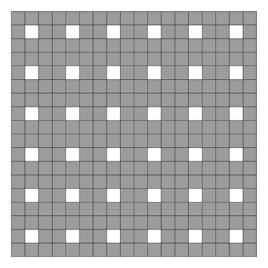
Figure 4: An $18\times 18$ XY lattice in which the $\beta$ cells form an ordered array: $\beta$ cells (white squares) are immersed in a background of $\alpha$ cells (gray squares). Each XY cell corresponds to an area of $\xi_{0}\times\xi_{0}$, and contains four atomic sites.

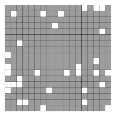
Figure 5: An $18\times 18$ XY lattice with a disordered arrangement of $\beta$ cells (white squares) immersed in a background of $\alpha$ cells (gray squares). Each cell corresponds to an area of $\xi_{0}\times\xi_{0}$, and contains four atomic sites. This Figure contains a particular realization of disorder. Density of states results for disordered systems are averaged over five different disorder realizations.

In Figs.  4 and 5, we show representative ordered and disordered arrangements of $\alpha$ and $\beta$ cells (for an $18\times 18$ XY lattice), similar to those used in the calculations of Fig. 3(a) and 3(b). In our density of states calculations for disordered arrangements, we typically average over about five realizations of the disorder, and use $24\times 24$ XY lattices rather than the $18\times 18$ shown in the schematic picture.

In Fig. 6, we show plots analogous to Fig. 3, but for a much larger concentration of $\beta$ cells ($c_{\beta}=0.89$). Part (a) shows results for an ordered array of $\alpha$ cells immersed in a background of $\beta$ cells. The simple, sharp peaks of the homogeneous $\beta$ case [dotted curves in Fig. 3(c) and Fig. 6(c)] are split into two sharp peaks at a slightly smaller energy, while the sharp peaks of the homogeneous alpha regions, [solid curve in Fig. 3(c)] become even sharper and shifted toward higher energies, leading to a reduction in the density of states near $\omega=0$. Also, in the inhomogeneous $\beta$ curve of Fig. 6(a), a weak second peak appears at the same energy as one of the peaks in the inhomogeneous $\alpha$ curve.

The case of a disordered distribution of $\alpha$ regions immersed in a background of $\beta$ regions is shown in Fig. 6 (b). The peaks of the curves corresponding to both the $\alpha$ and $\beta$ regions become lower and broader than in the homogeneous cases, Fig. 6(c). The peak in the $\beta$ curve occurs at approximately the same energy as in the homogeneous case. The corresponding inhomogeneous $\alpha$ peak, on the other hand, occurs at a higher energy relative to the homogeneous case.

V.2 Finite temperatures

We have carried out a finite-$T$ study for the system topology most similar to the experimental onelang_davis : a random distribution of $\beta$ regions immersed in a background of $\alpha$ regions. Calculated results for such a system at $T=0$ are shown in Fig. 3(b). Because more matrix diagonalizations are required at finite $T$ to obtain the relevant thermal averages, we work with $32\times 32$ atomic lattices, instead of the $48\times 48$ used at $T=0$. Since the computational time needed for one diagonalization scales with the linear size $L$ of the system like $L^{6}$, each diagonalization takes about one-tenth the time in these smaller system. Fortunately, the reduction of finite-size effects achieved by introducing a magnetic field leads to good results even for this relatively small system size. This can be seen by comparing the $t=0$ results in Fig. 7, which are obtained for a $32\times 32$ atomic lattice, to the corresponding results shown Fig. 3(b) for a $48\times 48$ atomic lattice.

Besides the partial densities of states, we calculate several additional quantities at finite $t$: the effective superfluid density $\gamma(t)$, the thermal- and space-averaged values of $|\psi|$ in the $\alpha$ and $\beta$ regions, and the relative fluctuations $\sigma_{|\psi|}$ of $|\psi|$ averaged over each of those regions.

We compute the superfluid density $\gamma$ by averaging the diagonal elements $\gamma_{\alpha\alpha}$ ($\alpha=x,y$) of the helicity modulus tensor $\hat{\gamma}$. Thus, we compute $\gamma=(\gamma_{xx}+\gamma_{yy})/2$, where ebner_stroud28

$$\gamma_{xx}=\frac{1}{M}\langle\sum_{\langle i,j\rangle}(x_{i}-x_{j})^{2}J_{XY,ij}\cos(\theta_{i}-\theta_{j})\rangle-\frac{1}{Mt}\langle[\sum_{\langle i,j\rangle}(x_{i}-x_{j})J_{XY,ij}\sin(\theta_{i}-\theta_{j})]^{2}\rangle$$

$$+\frac{1}{Mt}\langle\sum_{\langle i,j\rangle}(x_{i}-x_{j})J_{XY,ij}\sin(\theta_{i}-\theta_{j})\rangle^{2}.$$ (52)

Here $x_{i}$ is the $x$ coordinate of $i$th XY cell $i$, $M$ is the total number of XY cells, $J_{XY,ij}$ is the effective XY coupling between XY cells and is given by Eq. (34), $\theta_{i}$ is the phase of $\psi_{i}$ and $\langle\rangle$ denotes a canonical average. $\gamma_{yy}$ is defined by the analogous expression with $x_{i}$ replaced by $y_{i}$. In our computations, we have set the lattice constant $a_{XY}$ of the XY lattice to be unity.

The mean-square order parameter averaged over the $\alpha$ region is computed from

$$[\langle|\psi|^{2}\rangle]_{\alpha}=\frac{1}{M_{\alpha}}\sum_{i\in\alpha}\langle|\psi_{i}|^{2}\rangle,$$ (53)

where the sum is carried out over all $M_{\alpha}$ XY cells of type $\alpha$. $\left[\langle|\psi|^{2}\rangle\right]_{\beta}$ is defined similarly. The mean magnitude of the order parameter in the $\alpha$ and $\beta$ regions, denoted $[\langle|\psi|\rangle]_{\alpha}$ and $[\langle|\psi|\rangle]_{\beta}$, are defined by an equation analogous to eq. (53). We compute the relative fluctuations $[\sigma_{|\psi|}]_{\alpha}$ of $|\psi|$ within XY cells of type $\alpha$ from the definition

$$\left[\sigma_{|\psi|}\right]_{\alpha}=\left[\sqrt{\frac{\langle|\psi_{i}|^{2}\rangle-\langle|\psi_{i}|\rangle^{2}}{\langle|\psi_{i}|\rangle^{2}}}\right]_{\alpha},$$ (54)

where the triangular brackets denote a thermodynamic average, and $\left[...\right]_{\alpha}$ denotes a space average over the $\alpha$ sites. $\left[\sigma_{|\psi|}\right]_{\beta}$ is computed analogously. In systems with disorder, the square brackets denote a disorder average as well as a space average.

Fig. 7 shows the partial LDOS$(\omega,r)$ averaged over $\alpha$ and $\beta$ cells, at both $t=0$ and finite $t$. The systems shown have a fraction $c_{\beta}=0.1$ of $\beta$ sites randomly distributed. At $t=0$ the $\alpha$ regions show strong, sharp coherence peaks while the $\beta$ regions have a larger gap but lower and broader peaks. When the temperature is increased to $t=0.015$, the heights of both peaks are reduced, and their widths are increased, but the $\alpha$ peak is still quite sharp, because the system still has phase coherence. This temperature is still below the phase ordering temperature of $t_{c}\simeq 0.03$, as discussed below. As $t$ is increased still further, to $t=0.035$ and $t=0.055$, the two density of states peaks broaden still further, there is scarcely any residue of a gap in the density of states, and there is now no sign of a real coherence peak in either the $\alpha$ or the $\beta$ regions.

In Fig. 8, we show the superfluid density $\gamma(t)$, for the model just described but for various concentrations $c_{\beta}$ of the (randomly distributed) $\beta$ cells. For $c_{\beta}=0.1$, the phase-ordering transition temperature $t_{c}\sim 0.03$ in these units. Thus, of the plots in the previous Figure, two are below and two are above the phase-ordering transition.

In Figs. 9 and 10, we show the thermal, spatial, and disorder averages of $|\psi|$ over the $\alpha$ and $\beta$ regions, denoted $[\langle|\psi|\rangle]_{\alpha}$ and $[\langle|\psi|\rangle]_{\beta}$, while Figs. 11, and 12 show the corresponding averages of the root-mean-square fluctuations $\sigma_{|\psi|}$. A number of features deserve mention. First, the average $|\psi|$ is, of course, larger in the $\beta$ regions than in the $\alpha$ regions, but the root-mean-square fluctuations are comparable in each of the two regions. Second, the increases in the averages of $|\psi|$ above the phase-ordering temperature is an artifact of a Ginzburg-Landau free energy functional as we now explain in detail.

The asymptotic behavior of $|\psi|^{2}$ as $t\rightarrow\infty$, for homogeneous systems, can be obtained in the following way : At very high temperatures $t\gg t_{c0}$, the first term in (29) goes like $\sim|\psi|^{2}$, the second goes like $\sim|\psi|^{4}/t$ and the third (coupling) term goes like $\sim|\psi|^{2}/t$. We can then neglect the contribution of the third term, whence at large $t$ the XY cells are effectively decoupled. The thermal average of $|\psi|^{2}$ for an isolated cell is given by

$$\langle|\psi|^{2}\rangle=\frac{\int_{0}^{\infty}|\psi|d|\psi||\psi|^{2}\exp(-f|\psi|^{2}-g|\psi|^{4})}{\int_{0}^{\infty}|\psi|d|\psi|\exp(-f|\psi|^{2}-g|\psi|^{4})}.$$ (55)

In our case,

$$f=\frac{K_{1}}{t_{c0}^{3}\lambda^{2}(0)E_{0}}$$ (56)

and

$$g=\frac{K_{1}}{2\,(9.38)t_{c0}^{4}\lambda^{2}(0)E_{0}t}.$$ (57)

If $f$ and $g$ are real and positive, as in the present case, the integrals appearing in (55) can be carried out, with the result

$$\langle|\psi|^{2}\rangle=-\frac{f}{2g}+\frac{\exp(-f^{2}/4g)}{\sqrt{g}\pi\text{erfc}\,\,(f/2\sqrt{g})}.$$ (58)

Here $\text{erfc}(z)=1-\text{erf}(z)$, $\text{erf}(z)$ being the gaussian error function. Using an asymptotic expansion arfken for $\text{erf}(f/2\sqrt{g}$), applicable when $f/\sqrt{g}>>1$ as in the present case, we can show that

$$\lim_{t\rightarrow\infty}\langle|\psi|^{2}\rangle\rightarrow 1/f.$$ (59)

Substituting $f$ from eq. (56) leads to

$$\lim_{t\rightarrow\infty}\langle|\psi|^{2}\rangle\rightarrow\frac{t_{c0}^{3}\lambda^{2}(0)E_{0}}{K_{1}}\simeq 0.6$$ (60)

where the last approximate equality is obtained using the parameters we have discussed above, namely $K_{1}\simeq 2866$ eV-$\AA^{2}$, $\lambda(0)$ = 1800 $\AA$, $t_{c0}=0.14$, $E_{0}=200$meV.

On the other hand, using eq. (35), we obtain

$$\lim_{t\rightarrow\ 0}\langle|\psi|^{2}\rangle\simeq 0.2$$ (61)

Thus, our model introduces an unphysical finite value of $\langle|\psi|^{2}\rangle$ at large $t$. This behavior has been observed in other studies of similar modelsbittner_janke , while in other investigations this feature is less obvious because of the parameters usedebner_stroud25 . In our case, since we are interested in temperatures $t<t_{c}<t_{c0}$ or $t\sim t_{c}<t_{c0}$, this unphysical high-temperature behavior should not be relevant to our calculations.

Our results for $\left[\langle|\psi|\rangle\right]_{\alpha}$ and $\left[\langle|\psi|\rangle\right]_{\beta}$ suggest an explanation for one feature in the plots of the LDOS (see Fig. 7). Namely, the $\beta$ peak generally occurs at higher $\omega$ than it would in a superconductor made entirely of $\beta$ material. This shift occurs because, when the $\beta$ and $\alpha$ regions are mixed, $\left[\langle|\psi|\rangle\right]_{\beta}$ is larger than its value in a homogeneous $\beta$ system (as we further discuss below). This behavior of $\left[\langle|\psi|\rangle\right]_{\beta}$ can be seen in Fig. 10, where this quantity is plotted for different values of $c_{\beta}$. Clearly, at low $t$, $|\psi|$ increases as $c_{\beta}$ decreases. For the homogeneous $\beta$ system, $|\psi(t=0)|=1.29$, as can be obtained directly from eq. (35); this value is shown as an open circle at $t=0$. This upward shift in the $\left[\langle|\psi|\rangle\right]_{\beta}$ would be difficult to measure, since a pure $\beta$ material may not exist.

The behavior of $\left[\langle|\psi|\rangle\right]_{\beta}$ has an analog, in our model, in the corresponding behavior in the $\alpha$ cells. Specifically, if $\alpha$ cells are the minority component in $\beta$ host, $\langle|\psi|\rangle$ tends to be substantially smaller than in pure $\alpha$ systems: the smaller the concentration $c_{\alpha}=1-c_{\beta}$, the smaller the value of $\langle|\psi|\rangle$ in those regions [see Fig. 9]. The behavior of $\langle|\psi|\rangle$ in both $\alpha$ and $\beta$ regions basically follows from our earlier discussion, according to which $|\psi|^{2}$ is larger in regions with a small gap.

VI Discussion

We have presented a phenomenological model for the temperature-dependent single-particle density of states in a BCS superconductor with a $d_{x^{2}-y^{2}}$ order parameter. Our model includes both inhomogeneities in the gap magnitude and fluctuations in the phase and amplitude of the gap. While some of these features have been included in previous models for the density of states (e. g. phase fluctuations in a homogeneous d-wave superconductor, inhomogeneities in the gap magnitude at $T=0$), our model is more general, and thus potentially more realistic for some cuprate superconductors.

Our main goal is to examine the properties of an inhomogeneous superconductor, including many effects which are likely to be significant in real cuprate materials. The amplitude and phase fluctuations are treated by a discretized Ginzburg-Landau free energy functional, while the density of states is obtained by solving the Bogoliubov-de Gennes equations for a superconductor with a tight-binding density of states and a $d_{x^{2}-y^{2}}$ energy gap.

In all our calculations, we have assumed that the superconductor has two types of regions: $\alpha$, with a small gap but a high superfluid density; and $\beta$, with a large gap and small superfluid density. This assumption appears consistent with many experiments on the high-T_c cuprates, especially in the underdoped regime lang_davis . If we assume that the minority component is of type $\beta$, embedded in an $\alpha$ host, we find that the local density of states at $T=0$ at the $\alpha$ sites has sharp coherence peaks, whereas that of the $\beta$ sites is substantially broadened. This behavior is similar to experiment lang_davis ; pan_davis .

This description applies to a disordered distribution of $\beta$ sites in an $\alpha$ host. If the $\beta$ sites are, instead, arranged on a lattice, the local density of states on the $\beta$ sites is sharper, but also has distinct oscillations as a function of energy. Since such oscillations are absent in experiments, the actual $\beta$ regions, if they exist as a minority component, are probably distributed randomly.

In the reverse case of $\alpha$ regions embedded randomly in a $\beta$ host, neither component has an extremely sharp density of states peak. While the $\alpha$ peak is still quite sharp, it is broader than the $\alpha$ peak in the $\beta$-minority case. This result suggests that, if one component occurs only as isolated regions, its minority status tends to broaden its coherence peaks.

Our results also show that the local density of states is strongly affected by phase fluctuations. This feature has already been found for a homogeneous d-wave superconductoreckl , but here we demonstrate it in an inhomogeneous superconductor. The most striking effect of finite $T$ is that the coherence peak in the $\alpha$ component disappears above the phase-ordering transition temperature $T_{c}$. The $\beta$ component does not show a coherence peak even at very low temperatures, but nonetheless this peak too is significantly broadened above $T_{c}$. For $T$ well above $T_{c}$, there is no appreciable gap in the local density of states either at the $\alpha$ or the $\beta$ sites.

Our calculations include thermal fluctuations in the amplitude as well as the phase of $\psi$. In general, thermal amplitude fluctuations seem to have only a minor influence on the local density of states. By contrast, the variations in $|\psi|$ due to quenched disorder (i. e., the presence of $\alpha$ and $\beta$ regions in our model) strongly affect the local density of states, as we have already described. To check on the influence of purely thermal amplitude fluctuations, we have calculated the density of states of a homogeneous $\alpha$ superconductor with both phase and amplitude fluctuations, and have compared this to a similar calculation with only phase fluctuations. We find that the additional presence of amplitude fluctuations has little effect on the density of states.

To smooth the local density of states, we include in our density of states calculations a magnetic field equal to a flux $hc/e$ in the entire sample area, following the method of Assaadassaad . This field greatly smooths the local density of states, which otherwise varies extremely sharply with energy, because of the many degenerate states of a finite sample at zero field. Our calculated density of states does, of course, correspond to a physical magnetic field, and thus differs slightly from that at zero field. For example, in a homogeneous system with a finite $d$-wave gap, the LDOS$(\omega)$ goes to zero as $|\omega|\rightarrow 0$. By contrast, at finite field, the LDOS approaches a constant value at low $|\omega|$. With no gap, our calculated DOS with nonzero field is indistinguishable from that of a conventional 2D tight-binding band (see Fig. 1), because the field is low (typically around 0.002 flux quanta per atomic unit cell). We conclude that the weak magnetic field very effectively smooths the calculated LDOS in a finite two-dimensional sample with a d-wave gap, but produces a density of states similar to that at zero field, except at very low $|\omega|$.

Although we have included this magnetic field in the Bogoliubov-de Gennes equations, we have omitted it from the Ginzburg-Landau free energy functional, which is thus that of a zero-field system. As we now discuss, we believe that this numerical scheme should indeed converge to the correct physical result for zero magnetic field in the limit of a large computational sample.

As noted earlier, we introduce the vector potential into the LDOS calculation in order to smooth the resulting density of states. In the limit of a large system, the effect of the vector potential, corresponding to a single quantum of flux, should become negligible, since the flux density becomes very small. This is already suggested by our calculated results for the two system sizes we consider (see Fig. 2 and the corresponding discussion). Even with a finite superconducting gap, the vector potential affects the LDOS very little, except at low energies; moreover, even this effect becomes smaller as the sample size increases. Therefore, in the limit of a large enough sample, our approach should give a very similar LDOS to one calculated with no vector potential. Hence, it is reasonable to use this approach in combination with a zero-field Ginzburg-Landau free energy functional to calculate the LDOS at finite temperatures.

If we were to introduce a similar field into the Ginzburg-Landau functional, we believe that it would have a substantial effect, not due to smoothing, on the phase ordering. There would be, not only the XY-like phase transition, as at zero field, but also additional phase fluctuations arising from the extra field-induced vortex. Since this extra vortex is absent at zero field, these effects would be irrelevant to the zero-field system we wish to model. By contrast, introducing a field into the Bogoliubov-de Gennes equations, as we do, provides desirable smoothing with little change in the calculated LDOS; moreover, even this slight change decreases with increasing sample size. Therefore, we believe that the best way to obtain a smooth LDOS at both zero and finite temperatures is to introduce the vector potential into the Bogoliubov-de Gennes equations, for smoothing purposes, but not to include it in the Ginzburg-Landau free energy functional. Our numerical results suggest that this procedure is indeed justified.

One feature of our numerical results may seem counterintuitive. In our model, the $\alpha$ component is assumed to have a gap three times smaller than that of $\beta$, but has a larger local superfluid density, i. e., a smaller penetration depth. We then find that the gap in the $\alpha$ region is smaller in a two-component system with both $\alpha$ and $\beta$ regions, than it is in a pure $\alpha$ system. This counterintuitive result, however, emerges naturally from our discrete Ginzburg-Landau model, which is minimized if the quantities $\Delta_{i}/(\lambda_{i}(0)T_{c0i})$ are equal. For our model, $\lambda_{i}(0)$ is smaller in the small-gap material. It would be of interest if experimental evidence of this behavior were found in a real material.

In our calculation, the LDOS is obtained from a Bogoliubov-de Gennes Hamiltonian whose parameters are determined by the Ginzburg-Landau functional. In fact, it should be possible to proceed in the opposite direction, and obtain the parameters of the functional from the LDOS. Specifically, the energy required to change a phase difference by a given amount depends on an integral over the LDOS. Thus, the calculation we have presented in this paper can, in principle, be made fully self-consistent.

VII Acknowledgments

We are grateful for support through the National Science Foundation grant DMR04-13395. The computations described here were carried out through a grant of computing time from the Ohio Supercomputer Center. We thank E. Carlson, S. Kivelson, M. Randeria, N. Trivedi, R. Sensarma, D. Tanaskovic, and K. Kobayashi for valuable discussions.

Figure 1: Zero temperature density of states DOS$(\omega)$ versus energy $\omega$ for three homogeneous systems described by mean-field transition temperatures $t_{c0}=0$, $t_{c0}=0.14$, and $t_{c0}=0.42$. Simulations were carried out on $48\times 48$ atomic lattices, with a magnetic field included, as described in the text, to reduce finite size effects. Energies $\omega$ are given in units of $t_{hop}$.

Figure 2: Comparison of the $T=0$ DOS of a small system ($32\times 32$ atomic lattice) containing one quantum of magnetic field ($q=1$) to that of a larger ($48\times 48$) system with no magnetic field ($q=0$). Both systems are homogeneous with $t_{c0}=0.14$. Except at very low energies, the magnetic field produces little change in the shape of the curve.

Figure 3: Comparison of the zero temperature DOS of mixed $\alpha$-$\beta$ systems (a) and (b), and pure systems (c). In the mixed systems, $c_{\beta}=0.11$ is the concentration of $\beta$ cells ($t_{c0}=0.42$), immersed in a background of $\alpha$ cells ($t_{c0}=0.14$). (a) Ordered array of $\beta$ cells; see Fig 4. (b) Disordered configuration of $\beta$ cells; see Fig 5. Curves are obtained by space-averaging LDOS$(\omega,r)$ over atomic sites within $\alpha$ or $\beta$ cells, respectively. In the disordered case, averages were also carried out over five different realizations of the disorder. (c) DOS$(\omega)$ for two pure systems containing only $\alpha$ and only $\beta$ cells. We use a $48\times 48$ atomic lattice; the size of an XY cell ($\alpha$ or $\beta$) is $2\times 2$.

Figure 6: Same as Fig. 3 but with a high concentration $c_{\beta}=0.89$ of $\beta$ cells in the mixed systems. The ordered configuration corresponds to an ordered arrangement of $\alpha$ cells within $\beta$.

Figure 7: Spatial average, at several different temperatures $t$, of the local density of states LDOS$(\omega,r)$ over two different types of cells: the $\alpha$-cells, where $t_{c0}=0.14$, and the $\beta$-cells, where $t_{c0}=0.42$. The $\beta$-cells occupy 10% ($c_{\beta}=0.1$) of the total area, while the $\alpha$-cells occupy the rest. The simulations were performed using a $32\times 32$ atomic lattice; the XY cells are $2\times 2$ atomic cells. The phase ordering temperature for this system is $t_{c}\approx 0.03$ (see the curve corresponding to $c_{\beta}=0.1$ in Fig. 8).

Figure 8: Superfluid density $\gamma(t)$ versus temperature $t$, for systems with different concentrations $c_{\beta}$ of $\beta$ cells distributed randomly over the atomic lattice. $\beta$ cells have $t_{c0}=0.42$, whereas $\alpha$ cells have $t_{c0}=0.14$, However, the coupling constant between two nearest neighbor-cells $\langle ij\rangle$ includes, at low $t$, a factor $1/\sqrt{t_{c0i}\,t_{c0j}}$, which results in a suppression of the superfluid density in systems with large concentrations of $\beta$ cells [see Eq. (43)].

Figure 9: Space, thermally, and disorder-averaged $\left[\langle|\psi|\rangle\right]_{\alpha}$, averaged over $\alpha$ cells, for systems with different concentrations $c_{\beta}$ of $\beta$ cells, as described in the caption of Fig. 8. In an $\alpha$ cell $t_{c0}=0.14$ while $t_{c0}=0.42$ in a $\beta$ cell.

Figure 10: Same as Fig. 9, but averaged over the $\beta$ cells.

Figure 11: Relative thermal fluctuations $[\sigma_{|\psi|}(t)]_{\alpha}$ of $|\psi|$, averaged over the $\alpha$ cells, for systems with different concentrations $c_{\beta}$ of $\beta$ as shown in Fig. 8.

Figure 12: Same as Fig. 11 but averaged over the $\beta$ cells.

References

- (1) T. Cren, D. Roditchev, W. Sacks, J. Klein, J.-B. Moussy, C. Deville-Cavellin, and M. Lagues, Phys. Rev. Lett 84, 147 (2000).
- (2) C. Howald, P. Fournier, and A. Kapitulnik, Phys. Rev. B 64, 100504(R) (2001).
- (3) S. H. Pan, J. P. O’Neal, R. L. Badzey, C. Chamon, H. Ding, J. R. Engelbrecht, Z. Wang, H. Eisaki, S. Uchida, A. K. Gupta, K.-W. Ng, E. W. Hudson, K. M. Lang, and J. C. Davis, Nature 413, 282 (2001).
- (4) K. M. Lang, V. Madhavan, J. E. Hoffman, E. W. Hudson, H. Eisaki, S. Uchida, and J. C. Davis, Nature 415, 412 (2002).
- (5) C. Howald, H. Eisaki, N. Kaneko, M. Greven, and A. Kapitulnik, Phys. Rev. B 67, 014533 (2003).
- (6) T. Kato, S. Okitsu, and H. Sakata, Phys. Rev. B 72, 144518 (2005).
- (7) A. C. Fang, L. Capriotti, D. J. Scalapino, S. A. Kivelson, N. Kaneko, M. Greven, and A. Kapitulnik, Phys. Rev. Lett. 96, 017007 (2006).
- (8) H. Mashima, N. Fukuo, Y. Matsumoto, G. Kinoda, T. Kondo, H. Ikuta, T. Hitosugi and T. Hasegawa, Phys. Rev. B 73, 060502(R) (2006).
- (9) Yogesh N. Joglekar, A. H. Castro Neto, and Alexander V. Balatsky, Phys. Rev. Lett. 92,037004 (2004).
- (10) D. J. Scalapino, T. Nunner, and P. J. Hirschfeld, Journal of Physics and Chemistry of Solids 67, 2006.
- (11) Jan Zaanen and Olle Gunnarsson, Phys. Rev. B 40, 7391 (1989).
- (12) V. J. Emery, S. A. Kivelson, and H. Q. Lin, Phys. Rev. Lett. 64, 475 (1990).
- (13) V. J. Emery and S. A. Kivelson, Physica C 209, 597 (1993).
- (14) U. Löw, V. J. Emery, K. Fabricius, and S. A. Kivelson, Phys. Rev. Lett. 72, 1918 (1994).
- (15) See V. J. Emery, S. A. Kivelson and J. M. Tranquada, Proc. Natl. Acad. Sci. USA 96, 8814 (1999).
- (16) Reza Jamei, Steven Kivelson, and Boris Spivak, Phys. Rev. Lett. 94, 056805 (2005).
- (17) Daniel Valdez-Balderas and David Stroud, Phys. Rev. B 72, 214501 (2005).
- (18) Ivar Martin and Alexander V. Balatsky, Physica C 357-360, 46 (2001).
- (19) Ziqiang Wang, Jan R. Engelbrecht, Shancai Wang, Hong Ding, and Shuheng H. Pan, Phys. Rev. B 65, 064509 (2002).
- (20) W. A. Atkinson, Phys. Rev. B 71, 024516 (2005).
- (21) Tamara S. Nunner, Brian M. Andersen, Ashot Melikyan, and P. J. Hirschfeld, Phys. Rev. Lett. 95, 177003 (2005).
- (22) A. Ghosal, M. Randeria, and N. Trivedi, Phys. Rev. Lett. 81, 3940 (1998); A. Ghosal, M. Randeria, and N. Trivedi, Phys. Rev. B65, 014501 (2002).
- (23) A. Ghosal, M. Randeria, and N. Trivedi, Phys. Rev. B63, 020505(R) (2000). Arti Garg, Mohit Randeria, and Nandini Trivedi, cond-mat/0609666.
- (24) Ming Cheng and W. P. Su, Phys. Rev. B 72, 094512 (2005).
- (25) Matthias Mayr, Gonzalo Alvarez, Adriana Moreo, and Elbio Dagotto, Phys. Rev. B 73, 014509 (2006).
- (26) R. Jamei, J. Robertson, E-A. Kim, A. Fang, A. Kapitulnik, and S. A. Kivelson, cond-mat/0608318.
- (27) T. Eckl, D. J. Scalapino, E. Arrigoni, and W. Hanke Phys. Rev. B 66, 140510(R) (2002).
- (28) Phenomenological phase-fluctuation model for the underdoped cuprates. Doctoral thesis, Universität Würzburg, Würzburg, 2004.
- (29) See, e. g., Michael Tinkham, Introduction to superconductivity, 2nd edition (Dover Publications, Mineola, New York, 1996).
- (30) P. G. de Gennes, Superconductivity of metals and alloys (Addison-Wesley, New York, 1989).
- (31) B. Muhlschlegel, D. J. Scalapino, and R. Denton, Phys. Rev. B 6, 1767 (1972).
- (32) Michael E. Fisher, Michael N. Barber, and David Jasnow, Phys. Rev. A 8, 1111 (1973).
- (33) G. Deutscher, Y. Imry, L. Gunther, Phys. Rev. B 10, 4598 (1974).
- (34) B. R. Patton, W. Lamb and D. Stroud, Inhomogeneous Superconductors–1979, AIP Conf. Proc. 58, edited by D. U. Gubser et al, pp. 13-22.
- (35) C. Ebner and D. Stroud, Phys. Rev. B 23, 6164 (1981).
- (36) C. Ebner and D. Stroud, Phys. Rev. B 25, 5711 (1982).
- (37) C. Ebner and D. Stroud, Phys. Rev. B 28, 5053 (1983).
- (38) C. Ebner and D. Stroud, Phys. Rev. B 39, 789 (1989).
- (39) A. K. Nguyen and A. Sudbo, Phys. Rev. B 60, 15307 (1999).
- (40) Wang Xu, Yong Ren and C. S. Ting, Phys. Rev. B 53, 12481 (1996).
- (41) J. J. Vicente Alvarez, Gustavo C. Buscaglia, and C. A. Balseiro, Phys. Rev. B 54, 16168 (1996).
- (42) Manuel V. Ramallo and Felix Vidal, Phys. Rev. B 59, 4475 (1999).
- (43) Yong Ren, Ji-Hai Xu, and C. S. Ting, Phys. Rev. Lett. 74, 3680 (1995).
- (44) G. Alvarez and H. Fort, Phys. Rev. B 64, 092506 (2001).
- (45) Elmar Bittner and Wolfhard Janke, Phys. Rev. Lett. 89, 130201 (2002).
- (46) Andrei Mourachkine, High-Temperature Superconductivity in the Cuprates (Kluwer Academic Publishers, 2002). See plots in pages 67 and 84.
- (47) M.E.J. Newman and G.T. Barkema, Monte Carlo Methods in Statistical Physics (Oxford: Clarendon Press, 1999.)
- (48) J. M. Thijssen, Computational physics (Cambridge Univ. Press, Cambridge, 1999).
- (49) E. Anderson, Z. Bai, C. Bischof, S. Blackford, J. Demmel, J. Dongarra, J. Du Croz, A. Greenbaum, S. Hammarling, A. McKenney, A. and D. Sorensen, LAPACK Users’ Guide, 3rd Ed., (Society for Industrial and Applied Mathematics, Philadelphia, PA, 1999).
- (50) F. F. Assaad Phys. Rev. B 65, 115104 (2002).
- (51) Wenbin Yu, K. H. Lee and D. Stroud, Phys. Rev. B 47, 5906 (1993).
- (52) Leon Van Hove Phys. Rev. 89, 1189 (1953).
- (53) J. Lages, P. D. Sacramento, and Z. Tesanovic, Phys. Rev. B 69, 094503 (2004).
- (54) George B. Arfken and Hans J. Weber, Mathematical Methods for Physicists (Academic Press, 1995).