Quantum master equation for electron transport through
quantum dots and single molecules

Abstract

A quantum master equation (QME) is derived for the many-body density matrix of an open current-carrying system weakly coupled to two metal leads. The dynamics and the steady-state properties of the system for arbitrary bias are studied using projection operator techniques, which keep track of number of electrons in the system. We show that coherences between system states with different number of electrons, $n$, (Fock space coherences) do not contribute to the transport to second order in system-lead coupling. However, coherences between states with the same $n$ may effect transport properties when the damping rate is of the order or faster then the system Bohr frequencies. For large bias, when all the system many-body states lie between the chemical potentials of the two leads, we recover previous results. In the rotating wave approximation (when the damping is slow compared to the Bohr frequencies of the system), the dynamics of populations and the coherences in the system eigenbasis are decoupled. The QME then reduces to a birth and death master equation for populations.

Submitted to Phy. Rev. B

I introduction

Electron transport through a quantum dot (QD) or a single molecule has recently received considerable experimental reed ; park ; dadosh ; umansky ; w-ho ; ohtani and theoretical nitzan ; hofer ; sautet-chem-rev ; di-carlo-rep-phys ; stafford ; ratner_nature ; smit attention. The progress in the fabrication of devices such as quantum dots (whose size and geometry can be controlled with high precision wiel ) or single molecule junctions, makes it possible to investigate quantum effects on transport and provides a test for methods of nonequilibrium statistical mechanics. In analogy with laser optical spectroscopy tannoudji ; mukamel , electron transport through a quantum system (QD or single molecule) can be used to probe its nonequilibrium properties through the current-voltage $(I/V)$ characteristics. The scattering matrix (SM) sm ; bruss-flensberg and the non-equilibrium Greens function (NEGF) gf ; haug-jauho ; datta-book methods have been used for predicting $I/V$ characteristics of quantum systems connected to two metal leads. Both theories are exact in their respective domains: SM is limited to elastic processes while the NEGF can treat both elastic and inelastic processes.
The quantum master equation (QME) approach is an alternative tool for studying the irreversible dynamics of quantum systems coupled to a macroscopic environment spohn ; haake ; breuer . Owing to its simple structure, it provides an intuitive understanding of the system dynamics and has been used in various fields such as quantum optics gardiner ; tannoudji , solid state physics weiss , and chemical dynamics mukamel . Recently, it has been applied to study electron tunneling through molecules or coupled quantum dots brune ; gurvitz ; rammer ; pedersen ; yan ; sven . Fransson and Rasander fransson have recently used a QME approach to study the rectification properties of a system of coupled QDs by analyzing the occupation of two-electron triplet states as a function of the ratio of the interdot coupling and the energy splitting between the two QDs.

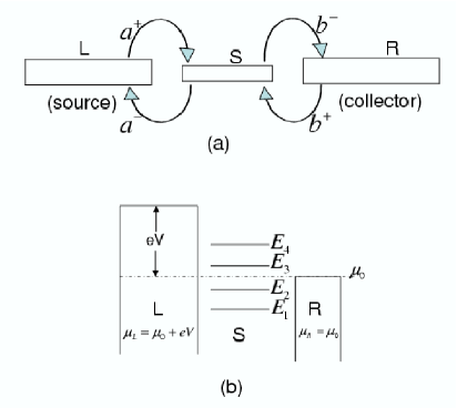
Gurvitz and Prager gurvitz were the first to derive a hierarchy of QMEs which keeps track of the number of electrons transferred from the source-lead to the collector-lead. Using this hierarchy they studied the effects of quantum coherence and Coulomb blockade on steady state electron transport in the high bias limit. In this limit all energy levels of the system are below the chemical potential of the left lead (source) and above the right lead (collector) (Fig. 1). The relevant Fermi functions for the left and the right leads are then unity and zero, respectively. Rammer $et$ $al$ rammer have used a QME to describe the direct tunneling (where the system never gets charged) in quantum junctions. Recently Pedersen and Wacker pedersen have generalized the standard rate equation and included approximately two-electron transfer processes by going beyond the second order perturbation in system-lead coupling.

In this paper, we use projection operator techniques to derive a new hierarchy of QME for the many-body density matrices $\rho^{n}$ representing the system with $n$ electrons. Electron transport through a quantum system is expressed in terms of the four processes describing the charging ($a^{+}$ and $b^{+}$) or discharging ($a^{-}$ and $b^{-}$) of the system at the left and the right leads (Fig. 1). Yan $et$ $al$ yan have used the same model to compute the steady-state current in the system by keeping track of the number of electrons at the collector-lead. In the limit of large bias, when the backward transport (corresponding to electron moving in the direction unfavored by the potential difference between the leads) can be neglected, we recover their results. Otherwise, it is necessary to identify $n$ as the number of electrons in the molecule, as done here. We solve our equations for a model system of two coupled quantum dots and study the effect of quantum coherences on electron transport. Coherence effects in quantum junctions have been studied in the past. Using the scattering matrix approach, Sautet $et$ $al$ sautet have found interference effects on the scanning tunneling microscopy images of molecules adsorbed on a metal surface. These effects arise from coherences between different open channels for the tunneling electrons.

The paper is organized as follows: In section II, we present the Hamiltonian and define a projection operator which keeps track of the system’s charge. We derive the QME and discuss its connection with earlier works. In section III, we show that under different approximations our QME recovers previous results and assumes a Lindblad form. Under the rotating wave approximation (in the system eigenbasis) the QME provides a very simple single particle picture of the dynamics of populations and coherences. In section IV, we study the dynamics, current and the charge of two coupled quantum dots (QD). In section V we present numerical results and discuss the effect of quantum coherences on the current. Conclusions are drawn is section VI.

II The Quantum master equation

The Hamiltonian of a quantum junction is given by the sum of the Hamiltonians for the isolated system, $H_{s}$, the left, $H_{L}$, and the right leads, $H_{R}$, and the lead-system coupling ($H_{T}$).

$$H = H_{s}+H_{L}+H_{R}+H_{T}$$ (1)

$$H_{s} = \sum_{s}\epsilon_{s}c_{s}^{\dagger}c_{s}$$ (2)

$$H_{L} = \sum_{l}\epsilon_{l}c_{l}^{\dagger}c_{l}$$ (3)

$$H_{R} = \sum_{r}\epsilon_{r}c_{r}^{\dagger}c_{r}$$ (4)

$$H_{T} = \sum_{s\nu}\left[T_{s\nu}c^{\dagger}_{s}c_{\nu}+h.c.\right]$$ (5)

where $s$, $l$ and $r$ represent system, left, and right lead orbitals, respectively, and $\nu=l,r$. $T_{sl}$ and $T_{sr}$ are the transfer coupling elements between the leads and the system. Direct coupling (tunneling) between the leads is neglectedrammer . $c^{\dagger}_{s}(c_{s})$, $c^{\dagger}_{l}(c_{l})$ and $c^{\dagger}_{r}(c_{r})$ are electron creation (annihilation) operators which satisfy the Fermi commutation relations

$$\{c_{k},c_{k^{\prime}}^{\dagger}\}=\delta_{kk^{\prime}},~{}~{}\{c^{\dagger}_{k},c^{\dagger}_{k^{\prime}}\}=\{c_{k},c_{k^{\prime}}\}=0,~{}~{}~{}~{}k,k^{\prime}=s,l,r$$ (6)

where $\{A,B\}=AB+BA$.

The many-electron eigenstates of the system form a ladder of manifolds: the $n^{\prime}$th manifold $|np\rangle$ contains the states ($p$) with $n$-electrons. Each interaction with the leads, Eq. (5), can change $n$ to $n\pm 1$. The total many-electron density matrix in Fock space can be expanded as,

$$\rho_{T}=\sum_{n,m,p,q}\rho^{pq}_{nm}|np\rangle\langle mq|.$$ (7)

The diagonal ($n=m$) blocks represent Fock space populations (FSP) of system states with $n$ electrons whereas the $n\neq m$ blocks are Fock space coherences (FSC). When the system is brought into contact with the leads, it is initially in the $n^{\prime}$th FSP block, $\rho_{nn}^{pq}$. As time evolves, FSC are developed, inducing transitions to other FSP blocks $n\pm 1$, $n\pm 2$, etc. At steady state, these blocks reach a stationary distribution and the current through the system can be calculated using time derivatives of the FSP.

Our first step is to derive a quantum master equation in Fock space which keeps track of the FSP and eliminates all FSC by incorporating them through relaxation kernelsbreuer . The Markovian master equation holds when the dephasing rates of FSP are large. In that case the steady state coherences are small, and progressively decrease for higher order coherences, i.e. as $|n-m|$ in Eq. (7) is increased. The dominant terms are $m=n\pm 1$ and the master equation rates can be calculated to second order in the coupling ($T$) with the leads. As the FSC dephasing rates decrease, one should calculate the rates to higher order in $T$. This problem is formally equivalent to the multiphoton excitation of molecules or atoms; the molecular states are divided into $n$-photon manifolds, and $n$-quantum coherences are eliminated to derive a Pauli master equation for the populations. Coupling with the radiation field in the rotating wave approximation plays the role of the coupling with the leads. The time-convolutionless projection operator techniques developed for multiphoton processes shaul-prl can be applied towards the calculation of molecular currents.

To derive a reduced description in the system space, we define the projection operators ${\cal P}_{n}$ which act on the many-body wave function $\Psi$rammer

$${\cal P}_{n}\Psi({\bf r}_{1},\cdots{\bf r}_{N})\equiv\theta_{n}({\bf r}_{1},\cdots{\bf r}_{N})\Psi({\bf r}_{1},\cdots{\bf r}_{N})\;,$$ (8)

where $\theta_{n}({\bf r}_{1},\cdots{\bf r}_{N})=1$ if precisely $n$ space-points belong to the system subspace and it vanishes otherwise. ${\cal P}_{n}$ is thus a Fock space projection operator onto states with $n$ electrons in the system. The projected many-body density matrix ($\rho^{n}$) onto the system subspace with $n$ electrons is defined as,

$$\rho^{n}\equiv\mbox{Tr}_{lead}\left\{{\cal P}_{n}\rho_{T}{\cal P}_{n}\right\}.$$ (9)

Note that by defining the projection operator for a fixed number of electrons in the system, we ignore the coherences between the leads and the system. The projection of the many-body density matrix can also be formulated in Liouville space using the projection superoperator (${\cal C}_{n}$) as ${\cal C}_{n}\rho_{T}=\rho^{n}\rho_{B}$, where $\rho_{B}$ is the density matrix of the leads (bath).

The QMEs for the projected many-body density matrices of the system is derived in Appendix A using second order perturbation theory in the system-lead coupling and by treating the two leads as infinite electron reservoirs:

$$\frac{\partial\rho^{n}(t)}{\partial t}=-i[H_{s},\rho^{n}(t)] + \sum_{ss^{\prime}}\left[\alpha_{ss^{\prime}}c_{s^{\prime}}\rho^{n+1}(t)c_{s}^{\dagger}-\beta_{ss^{\prime}}\rho^{n}(t)c_{s^{\prime}}c_{s}^{\dagger}\right.$$ (10)

$$- \left.\alpha_{ss^{\prime}}c_{s}^{\dagger}c_{s^{\prime}}\rho^{n}(t)+\beta_{ss^{\prime}}c_{s}^{\dagger}\rho^{n-1}(t)c_{s^{\prime}}+h.c.\right]\;,$$

with

$$\alpha_{ss^{\prime}} = \int_{0}^{\infty}d\tau e^{i\epsilon_{s^{\prime}}\tau}\alpha_{ss^{\prime}}(\tau)=\lim_{\eta\to 0}\sum_{\nu}\frac{T_{s\nu}T^{*}_{s^{\prime}\nu}(1-f_{\nu})}{\epsilon_{s^{\prime}}-\epsilon_{\nu}+i\eta}$$ (11)

$$\beta_{ss^{\prime}} = \int_{0}^{\infty}d\tau e^{i\epsilon_{s^{\prime}}\tau}\beta_{ss^{\prime}}(\tau)=\lim_{\eta\to 0}\sum_{\nu}\frac{T_{s\nu}T^{*}_{s^{\prime}\nu}f_{\nu}}{\epsilon_{s^{\prime}}-\epsilon_{\nu}+i\eta}\;.$$ (12)

where $f_{l}$ ($f_{r}$) is the Fermi distribution of the left (right) lead with chemical potential $\mu_{L}=\mu_{0}+eV$ ($\mu_{R}=\mu_{0}$) and $eV$ is the applied bias. $\alpha_{ss^{\prime}}(\tau)$’s and $\beta_{ss^{\prime}}(\tau)$’s are the lead correlation functions, Eq. (A), and have the symmetry

$$\alpha_{ss^{\prime}}^{*}(\tau)=\alpha_{s^{\prime}s}(-\tau)\ \ \;,\ \ \beta_{ss^{\prime}}^{*}(\tau)=\beta_{s^{\prime}s}(-\tau)\;.$$ (13)

Taking into account that the leads are macroscopic and have a continuous density of states, Eq. (A) gives

$$\sum_{\nu}e^{-i\epsilon_{\nu}\tau}T_{s\nu}T_{s^{\prime}\nu}^{*}f_{\nu}\to\sum_{X}\int d\epsilon\;n_{X}(\epsilon)e^{-i\epsilon\tau}T_{s}^{(X)}(\epsilon)T_{s^{\prime}}^{(X)*}(\epsilon)f_{X}(\epsilon)\;,$$ (14)

where $X=L,R$ and $n_{X}$ is the density of states of lead $X$. Substituting the relation

$$\int_{0}^{\infty}d\tau e^{i\omega\tau}=\pi\delta(\omega)+{\rm i}{\cal P}\frac{1}{\omega}\;,$$ (15)

in Eqs. (11) we obtain

$$\alpha_{ss^{\prime}} = \sum_{X}\alpha_{ss^{\prime}}^{(X)}\ \ ;\ \ \beta_{ss^{\prime}}=\sum_{X}\beta_{ss^{\prime}}^{(X)}$$ (16)

$$\alpha_{ss^{\prime}}^{(X)} = \pi n_{X}(\epsilon_{s^{\prime}})T_{s}^{(X)}(\epsilon_{s^{\prime}})T^{(X)*}_{s^{\prime}}(\epsilon_{s^{\prime}})(1-f_{X}(\epsilon_{s^{\prime}}))+{\rm i}\int d\epsilon{\cal P}\frac{n_{X}(\epsilon)T_{s}^{(X)}(\epsilon)T^{(X)*}_{s^{\prime}}(\epsilon)(1-f_{X}(\epsilon))}{\epsilon_{s^{\prime}}-\epsilon}$$ (17)

$$\beta_{ss^{\prime}}^{(X)} = \pi n_{X}(\epsilon_{s^{\prime}})T_{s}^{(X)}(\epsilon_{s^{\prime}})T^{(X)*}_{s^{\prime}}(\epsilon_{s^{\prime}})f_{X}(\epsilon_{s^{\prime}})+{\rm i}\int d\epsilon{\cal P}\frac{n_{X}(\epsilon)T_{s}^{(X)}(\epsilon)T^{(X)*}_{s^{\prime}}(\epsilon)f_{X}(\epsilon)}{\epsilon_{s^{\prime}}-\epsilon}\;.$$ (18)

The real parts of $\alpha_{ss^{\prime}}$ and $\beta_{ss^{\prime}}$ define the system to leads and leads to system electron transfer rates, respectively. The imaginary parts represent level shifts. $\Re\alpha_{ss}^{(X)}$ is the rate with which electrons are transferred from the $s^{\prime}$th system orbital to lead $X$ while $\Re\beta_{ss}^{(X)}$ is the transfer rate of electrons from lead $X$ to the system orbital. Thus $\Re\alpha_{ss^{\prime}}$ and $\Re\beta_{ss^{\prime}}$ are associated with the processes where the system undergoes transition between many-body states which differ by a single electron. When the external bias is large enough so that $f_{L}(\epsilon_{s})=1$ and $f_{R}(\epsilon_{s})=0$, $\Re\alpha^{L}_{ss^{\prime}}=\Re\beta^{R}_{ss^{\prime}}=0$. This means that the backward flow of electrons (electrons moving against the applied bias) from the right to the left lead vanishes and that each time the number of electrons in the system decreases it corresponds to an electron tunneling to the right lead. Keeping track of the electrons in the system is therefore directly related to counting of the electrons collected in the right lead. In such case, we recover the result of Yan yan . However, in general it is essential to recognize that $\rho^{n}$ is the density matrix of the system with $n$ electrons residing in the system. When $n$ decreases by one, the electron will, with a higher probability, be collected in the right lead, but could also be collected in the left lead. The effect of this last process on the dynamics is not captured in the other QME yan but is made clear in our QME by the use of projection operators.

To appreciate the reduction involved in the QME, let us consider a system with $n$ electrons and $M$$(n\leq M)$ orbitals. The number of $n$-electron many-body states is then $C^{M}_{n}=\frac{M!}{(M-n)!n!}$ and the total number of many body states is $N_{\rm tot}(M)=\sum_{n=0}^{M}C^{M}_{n}=2^{M}$. The full many-body density matrix is $N_{\rm tot}(M)\times N_{\rm tot}(M)$. Because the FSC between many-body states with different $n$ are eliminated, the size of the reduced many-body density matrix is $\sum_{n=0}^{M}(C^{M}_{n})^{2}$. In the full Liouville space of the system, the many-body density matrix is an $N_{\rm tot}^{2}(M)$ vector. However, the projected many-body density matrix $\rho_{s}=\sum_{n}\rho^{n}$ in this space contains $(\sum_{n=0}^{M}C^{M}_{n})^{2}-\sum_{n=0}^{M}(C^{M}_{n})^{2}$ elements which are zero. Our QME is therefore defined in a reduced many-body Liouville space of the system where the FSC have been eliminated.

III Limiting cases and the Lindblad form

III.1 High bias limit

When all many-body states of the system lie within the chemical potentials of two leads, the reverse electron tunneling can be ignored since the Fermi functions for the left and right leads are $f_{L}(\epsilon_{s})=1$ and $f_{R}(\epsilon_{s})=0$ gurvitz ; sprekeler . If we neglect the principal parts in Eqs. (17) and (18), the matrices $\alpha$ and $\beta$ become hermitian. In this case, since $\alpha_{ss^{\prime}}^{L}=\beta_{ss^{\prime}}^{R}=0$ we have $\alpha_{ss^{\prime}}=n^{R}T_{s}^{R}T_{s^{\prime}}^{R}$ and $\beta_{ss^{\prime}}=n^{L}T_{s}^{L}T_{s^{\prime}}^{L}$. We have further ignored the energy dependence of $\alpha_{ss^{\prime}}$ and $\beta_{ss^{\prime}}$. Defining $B_{s}=\sqrt{n^{R}}T^{R}_{s}c_{s}$, $D_{s}=\sqrt{n^{L}}{T^{L}_{s}}^{*}c_{s}^{\dagger}$ and summing the QME (10) over $n$ so that $\rho(t)=\sum_{n}\rho^{n}(t)$ sum-over-n , we get

$$\dot{\rho} = -i[H_{s},\rho]+\sum_{ss^{\prime}}\left[2B_{s^{\prime}}\rho B_{s}^{\dagger}-B_{s}^{\dagger}B_{s^{\prime}}\rho-\rho B_{s^{\prime}}^{\dagger}B_{s}+2D_{s^{\prime}}\rho D_{s}^{\dagger}-D_{s}^{\dagger}D_{s^{\prime}}\rho-\rho(t)D_{s^{\prime}}^{\dagger}D_{s}\right]\;.$$ (19)

Keeping in mind that FSC are zero so that terms, such as $B_{s^{\prime}}\rho D_{s}^{\dagger}$, $B_{s^{\prime}}^{\dagger}\rho B_{s}$, etc. which lead to FSC, vanish, Eq. (19) assumes a Lindblad form,

$$\dot{\rho}=-i[H_{s},\rho]+\sum_{ss^{\prime}}\left[2A_{s^{\prime}}\rho A_{s}^{\dagger}-A_{s}^{\dagger}A_{s^{\prime}}\rho-\rho A_{s^{\prime}}^{\dagger}A_{s}\right],$$ (20)

where $A_{s}=B_{s}+D_{s}=\sqrt{n^{R}}T^{R}_{s}c_{s}+\sqrt{n^{L}}{T^{L}_{s}}^{*}c_{s}^{\dagger}$. Gurvitz gurvitz has studied the effect of coherences in a QD system connected in series in the high bias limit. In Appendix B we show that Our QME reduces to Gurvitz equations in this limit.

III.2 The Rotating Wave Approximation

When the interaction between the system and the leads is weak enough for the damping effects to be slow compared to the Bohr frequencies of the system, we can simplify Eq. (10) by using the rotating wave approximation breuer ; gardiner ; tannoudji . This approximation is often performed on the Markovian form of the Redfield equation in order to prevent the possible breakdown of positivity spohn ; tannor1 ; tannor2 ; breuer due to the nonMarkovian effects of the initial dynamicshaakeslip ; suarez ; gaspard . Transforming the master equation to the interaction picture, we get Eq. (62) with the Markovian approximation $\int_{0}^{t}d\tau\to\int_{0}^{\infty}d\tau$ and with the Born approximation ${\tilde{\rho}}^{n}(t-\tau)\to{\tilde{\rho}}^{n}(t)$. Since the damping rate of the density matrix in the interaction representation is small compared to the Bohr frequencies of the system, we can time average ($\lim_{T\to\infty}\frac{1}{T}\int_{0}^{T}dt$) the fast oscillations due to the terms $e^{i\epsilon_{ss^{\prime}}t}$ in Eq. (62). This allows to eliminate the nondiagonal elements of the correlation function matrices [$\alpha_{ss^{\prime}}=\alpha_{ss}\delta_{ss^{\prime}}$ and $\beta_{ss^{\prime}}=\beta_{ss}\delta_{ss^{\prime}}$]. Going back to the Schrodinger picture, our equation reads

$$\dot{\rho}^{n}=-i[H_{s},\rho^{n}]+\sum_{s}\left[\alpha_{ss}c_{s}\rho^{n+1}c_{s}^{\dagger}-\beta_{ss}\rho^{n}c_{s}c_{s}^{\dagger}-\alpha_{ss}c_{s}^{\dagger}c_{s}\rho^{n}+\beta_{ss}c_{s}^{\dagger}\rho^{n-1}c_{s}+h.c.\right]\;.$$ (21)

By projecting this equation into the reduced Fock basis, we find that the coherences are decoupled from the populations.
When the level shifts in Eqs. (17) and (18) are ignored, the matrices $\alpha$ and $\beta$ in Eq. (21) become Hermitian. Using $a_{s}=\sqrt{\alpha_{ss}}c_{s}$, $b_{s}=\sqrt{\beta_{ss}}c_{s}^{\dagger}$ and following the same steps as in case of high bias limit, we find that Eq. (21) when summed over $n$ is of a Lindblad form similar to Eq. (20):

$$\dot{\rho}=-i[H_{s},\rho]+\sum_{s}\left[2A_{s}\rho A_{s}^{\dagger}-A_{s}^{\dagger}A_{s}\rho-\rho A_{s}^{\dagger}A_{s}\right]\;.$$ (22)

Note that in the RWA, since the matrices $\alpha$ and $\beta$ are diagonal, the sum in Eq. (22) only runs over one index $s$ and, unlike the high bias case, the coupling coefficients $T_{ss}^{L(R)}$ can be energy dependent.
Thus, we conclude that both in the high bias limit and the RWA form our QME are of Lindblad form which guarantees to preserve the positivity and the hermiticity of the density matrix.

The dynamics of the reduced many-body density matrix [Eq. (21)] can be expressed in terms of the time evolution of the single-orbital density matrix $\rho_{s}$ corresponding to the $s$th orbital.

$$\dot{\rho}_{s} = -i\epsilon_{ss}[c_{s}^{\dagger}c_{s},\rho_{s}]+2\Re\alpha_{ss}c_{s}\rho_{s}c_{s}^{\dagger}+2\Re\beta_{ss}c_{s}^{\dagger}\rho_{s}c_{s}$$

$$-\alpha_{ss}c_{s}^{\dagger}c_{s}\rho_{s}-\alpha_{ss}^{*}\rho_{s}c_{s}^{\dagger}c_{s}-\beta_{ss}^{*}c_{s}c_{s}^{\dagger}\rho_{s}-\beta_{ss}\rho_{s}c_{s}c_{s}^{\dagger}\;,$$

This means that if the initial many-body density matrix in Fock space is a direct product of single-orbital density matrices $\rho=\rho_{1}\otimes\rho_{2}\otimes\cdots\otimes\rho_{M}$ it will remain so at all times. However, even if the initial many-body density matrix is not a tensor product, since in the RWA, the r.h.s. of Eq. (21)is a sum of contributions from various orbitals, we can still factorize the many-body populations as products of single-orbital populations

$$\langle n_{1}\cdots n_{M}|\rho|n_{1}\cdots n_{M}\rangle=\prod_{s=1}^{M}p_{n_{s}}^{(s)}$$ (23)

where $p_{n_{s}}^{(s)}=\langle n_{s}|\rho_{s}|n_{s}\rangle$ and $n_{s}$ is the occupation of $s$th orbital. The dynamics of the single-orbital occupation is given by

$$\left(\begin{array}[]{c}\dot{p}_{1}^{(s)}\\ \dot{p}_{0}^{(s)}\end{array}\right)=2\left(\begin{array}[]{cc}-\Re\alpha_{ss}&\Re\beta_{ss}\\ \Re\alpha_{ss}&-\Re\beta_{ss}\end{array}\right)\left(\begin{array}[]{c}p_{1}^{(s)}\\ p_{0}^{(s)}\end{array}\right)\;.$$ (30)

We can readily find the steady state distribution

$$p_{1}^{(s)}=\frac{\Re\beta_{ss}}{\Re\alpha_{ss}+\Re\beta_{ss}}\ \ ;\ \ p_{0}^{(s)}=\frac{\Re\alpha_{ss}}{\Re\alpha_{ss}+\Re\beta_{ss}}\;.$$ (31)

The many-body steady state distribution can be directly obtained using (23) and (31).

IV Model Calculations

We consider a system of two coupled quantum dots (QD) each having a single orbital in the energy range between the chemical potentials of the left ($\mu_{L}$) and the right ($\mu_{R}$) leads. Depending on the interdot coupling, the system orbitals may either be localized (weak coupling) or delocalized (strong coupling). The system Hamiltonian is

$$H_{s}=\epsilon_{1}c_{1}^{\dagger}c_{1}+\epsilon_{2}c_{2}^{\dagger}c_{2}\;,$$ (32)

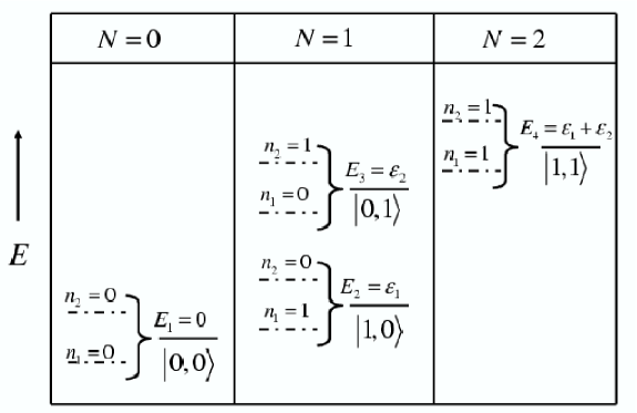
where $\epsilon_{1}$ and $\epsilon_{2}$ are system orbital energies and we have ignored the charging effects due to electron-electron interactions (Coulomb-blockade) bruder ; gurvitz in the system. We denote the many-body states $\{|n_{1},n_{2}\rangle\}$, where $n_{1}$ and $n_{2}$ are the occupation of the system orbitals $1$ and $2$, respectively. They can have values $0$ or $1$. The many-body level scheme is sketched in Fig. 2. The full system density matrix has $16$ components. In the reduced space, where FSC are eliminated, it has only six components. We order the vector given by the density matrix in the reduced space as $\rho=(\rho_{00,00}\;,\;\rho_{01,01}\;,\;\rho_{10,10}\;,\;\rho_{11,11}\;,\;\rho_{01,10}\;,\;\rho_{10,01})$. Our QME, Eq. (10), therefore reads

$$\dot{\rho}=\hat{{\cal M}}\rho$$ (33)

with

$$\hat{{\cal M}}=\left(\begin{array}[]{cccccc}-2\Re(\beta_{11}+\beta_{22})&2\Re\alpha_{22}&2\Re\alpha_{11}&0&\alpha_{12}+\alpha_{21}^{*}&\alpha_{21}+\alpha_{12}^{*}\\ 2\Re\beta_{22}&-2\Re(\alpha_{22}+\beta_{11})&0&2\Re\alpha_{11}&-\alpha_{21}^{*}+\beta_{12}&-\alpha_{21}-\beta_{12}^{*}\\ 2\Re\beta_{11}&0&-2\Re(\alpha_{11}+\beta_{22})&2\Re\alpha_{22}&-\alpha_{12}+\beta_{21}^{*}&-\alpha_{12}^{*}+\beta_{21}\\ 0&2\Re\beta_{11}&2\Re\beta_{22}&-2\Re(\alpha_{11}+\alpha_{22})&-\beta_{12}-\beta_{21}^{*}&-\beta_{12}^{*}-\beta_{21}\\ \beta_{21}+\beta_{12}^{*}&-\alpha_{12}^{*}+\beta_{21}&-\alpha_{21}+\beta_{12}^{*}&-\alpha_{21}-\alpha_{12}^{*}&-{\cal X}&0\\ \beta_{12}+\beta_{21}^{*}&-\alpha_{12}+\beta_{21}^{*}&-\alpha_{21}^{*}+\beta_{12}&-\alpha_{12}-\alpha_{21}^{*}&0&-{\cal X}^{*}\end{array}\right),$$ (40)

and ${\cal X}=\alpha_{11}^{*}+\beta_{11}^{*}+\alpha_{22}+\beta_{22}s+i(\epsilon_{1}-\epsilon_{2})$. At steady state ($\dot{\rho}=0$) this equation can be transformed into a $4\times 4$ matrix equation for populations alone by including the effect of coherences into modified rates sprekeler . In the present work we do not consider the spin polarization of the electrons which has been used to study Pauli blockade fransson and magnetotransport gurvitz1 in QDs. Recently Gurvitz $et$ $al$ gurvitz1 have derived a QME to study the spin dependent coherence effects on electron transfer through a single QD. We notice that, in the high bias limit, our Eqs. (33) and (40) are identical to their Eqs. (21) for the case of a single spin state (Sec. C in Ref. gurvitz1 ).

The total charge of the system at time $t$ is given by

$$Q(t)=e\ll N|\rho(t)\gg=e{\rm Tr}N\rho(t)$$ (41)

where $N=\sum_{s}c_{s}^{\dagger}c_{s}$ is the number operator. The rate of change of the system charge is given by

$$\dot{Q}(t)=I_{L}(t)+I_{R}(t)\;,$$ (42)

where $I_{L}$ and $I_{R}$ are the currents from the left and the right leads

$$I_{X}(t)=e\ll N|\hat{\cal M}_{X}|\rho(t)\gg,~{}~{}~{}~{}~{}~{}~{}X=L,R\;.$$ (43)

$\hat{\cal M}_{X}$ is the contribution to the matrix $\hat{\cal M}$ from lead $X$ so that $\hat{\cal M}=\hat{\cal M}_{L}+\hat{\cal M}_{R}$ ($\hat{\cal M}_{X}$ only contains terms in (40) corresponding to $X$ lead). Since $\alpha(\beta)$ is related to the outflux (influx) of electrons from (to) the system, we can further split the current as $I_{X}=I^{in}_{X}+I^{out}_{X}$, where

$$I^{in}_{X}(t) = e\ll N|\hat{\cal M}_{X}(\beta)|\rho(t)\gg$$

$$I^{out}_{X}(t) = e\ll N|\hat{\cal M}_{X}(\alpha)|\rho(t)\gg\;.$$ (44)

$\hat{\cal M}_{X}(\alpha)$ $[\hat{\cal M}_{X}(\beta)]$ contains only those terms in (40) involving $\alpha^{(X)}$ [$\beta^{(X)}$]. At steady state $(t\to\infty)$, the currents from the left and from the right leads must be equal and opposite in sign, and the steady-state current is given by $I_{s}=I_{L}=-I_{R}$.
We solve Eq. (33), by diagonalizing the matrix ${\cal\hat{M}}$.

$$|\rho\gg(t)=\sum_{\eta}C_{\eta}e^{\xi_{\eta}t}|\eta\gg\;,$$ (45)

where $\xi_{\eta}$ ($|\eta\gg$) are the eigenvalues (eigenvectors) of ${\cal\hat{M}}$ and $C_{\eta}=\ll\eta|\rho(0)\gg$. In the RWA [see Eq. (21)] the off-diagonal terms $\alpha_{ss^{\prime}}$ and $\beta_{ss^{\prime}}$ are neglected and the population dynamics of Eq. (40) is then independent of the coherences and can be obtained analytically (see Appendix C).

The steady state currents $I^{in}$ and $I^{out}$ are obtained from Eqs. (IV) and (C)

$$I_{L}^{in} = 2e\sum_{s=1,2}\frac{a^{L}_{ss}(\epsilon_{s})\alpha_{ss}}{a^{L}_{ss}(\epsilon_{s})+a^{R}_{ss}(\epsilon_{s})}f_{L}(\epsilon_{s})$$

$$I_{L}^{out} = -2e\sum_{s=1,2}\frac{a^{L}_{ss}(\epsilon_{s})\beta_{ss}}{a^{L}_{ss}(\epsilon_{s})+a^{R}_{ss}(\epsilon_{s})}(1-f_{L}(\epsilon_{s}))\;,$$ (46)

where $a^{X}_{ss}=\pi n_{X}|T^{X}_{s}(\epsilon_{s})|^{2}$. Similar expressions can be obtained for the currents $I^{in}_{R}$ and $I^{out}_{R}$ by interchanging $L$ and $R$ in Eq. (IV). Note that at steady state $\hat{{\cal M}}_{L}\rho=-\hat{{\cal M}}_{R}{\rho}$ so that $\dot{\rho}=0$. Of course $\hat{{\cal M}}_{L}(\alpha)\rho\neq-\hat{{\cal M}}_{L}(\beta){\rho}$. At steady state $I_{L}=-I_{R}$. We can therefore write for the steady state current $I_{s}=xI_{L}+(x-1)I_{R}$ for arbitrary $x$. By choosing $x=a^{R}_{ss}(\epsilon_{s})/(a^{L}_{ss}(\epsilon_{s})+a^{R}_{ss}(\epsilon_{s}))$, $I_{s}$ can be written in a symmetric form yan ; datta-book ; haug-jauho

$$I_{s}=2e\sum_{s}\frac{a^{L}_{ss}(\epsilon_{s})a^{R}_{ss}(\epsilon_{s})}{a^{L}_{ss}(\epsilon_{s})+a^{R}_{ss}(\epsilon_{s})}[f_{L}(\epsilon_{s})-f_{R}(\epsilon_{s})]\;.$$ (47)

Since in the RWA the many-body density matrix is given by a product of single-orbital density matrices, the total steady state current is the sum of contributions from various orbitals. Note that Eq.(47) gives the steady state current within the RWA, which ignores the effects of coherences. In the model calculations presented in the next section, we shall discuss these results and the effects of coherences.

V Numerical results

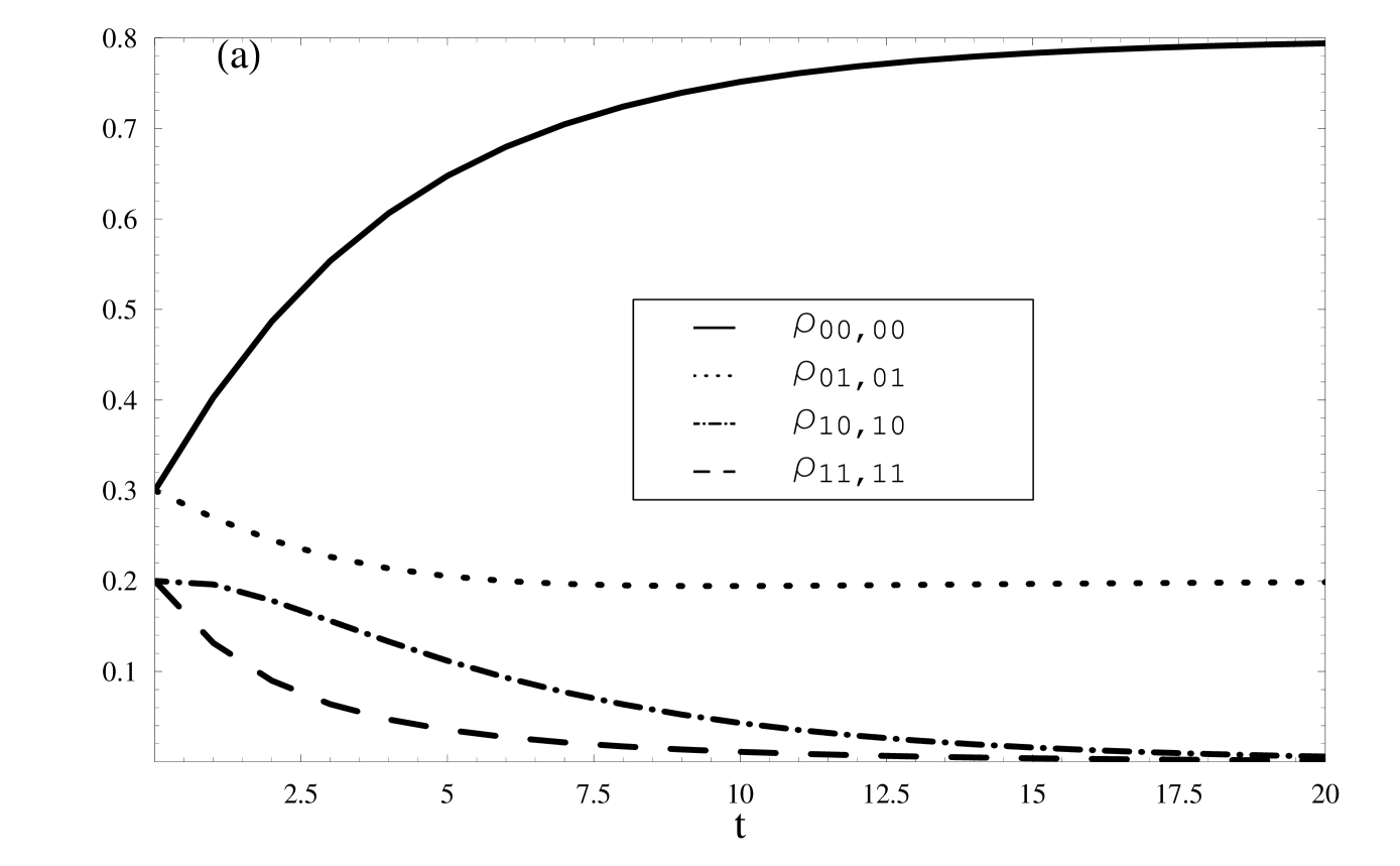
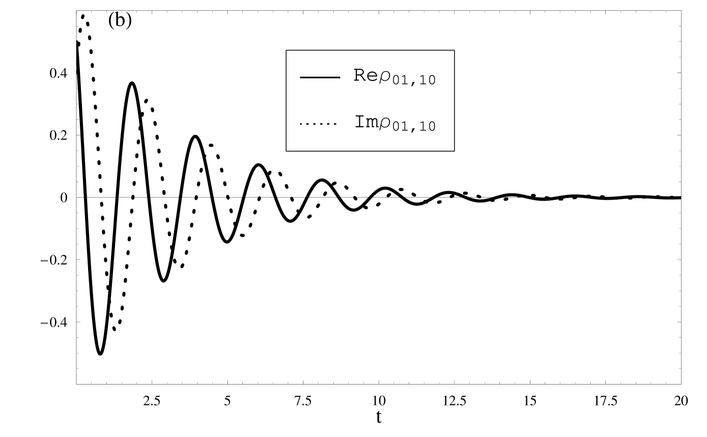
We first solve Eq. (33) for the time-dependent density matrix in terms of the eigenvalues and eigenvectors of the matrix ${\cal M}$ [see Eq. (45)]. We fix the system orbital energies, $\epsilon_{1}=5eV$ and $\epsilon_{2}=2eV$ and the temperature $k_{B}T=.2eV$. In Fig. 3 we display the eigenvalue spectrum of ${\cal\hat{M}}$. All eigenvalues have a real negative part representing an exponential decay. At long time, the system approaches the steady state corresponding to the zero eigenvalue. The two complex eigenvalues describe the two coherences.

The time evolution of the populations [Eqs. 45] and coherences [Eqs. 96] is shown in Figs. 4a and 4b, respectively. The two are decoupled in the RWA. Coherences show a damped oscillatory behavior and vanish at long times. The populations evolve exponentially and reach a steady state distribution described by the eigenvector with zero eigenvalue.

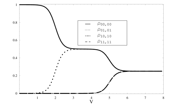
For large bias ($eV>\epsilon_{1}$) and identical left and right couplings ($T^{L}_{s}=T^{R}_{s}$), all many-body states have the same occupation. This is shown in Fig. 5. We assume that the chemical potential for the left lead increases with the bias while the right lead is held fixed at the Fermi energy $\mu_{0}$. When the bias is switched on, electrons start to move from the left to the right lead through the system. For $\mu_{0}\leq 0$ and $V=0$ there are no electrons in the system and the probability to find the system in the state $|00\rangle$ is one. This probability decreases as $V$ is increased. Thus $\rho_{00}$ decreases with increasing bias. As the bias is scanned across higher energies, electrons start to fill the system. This gives rise to the step-wise change in the population in Fig. 5. As long as $eV<\epsilon_{1}$, only states $|00\rangle$ and $|01\rangle$ are populated. For $eV\geq\epsilon_{1}$, both system orbitals lie between $\mu_{0}$ and $\mu_{0}+eV$, and all many-body states are equally populated.

The steady state $I/V$ characteristics of the system computed using Eqs. (IV) and (47) are depicted in Fig. 6. The black solid curve shows the total current computed using Eq. (47) and dots (dash-dot) show the current $I^{in}_{L}$ ($I^{out}_{L}$). We note that $I^{out}_{L}$ is significant only at resonant energies where $eV+\mu_{0}=\epsilon_{s}$. This can be explained as follows: when $\mu_{0}+eV<\epsilon_{s}$, there are no electrons in the $s^{\prime}$th orbital and hence $I^{out}_{L}=0$. For $\mu_{0}+eV>\epsilon_{s}$, in order to move from $s^{\prime}$th orbital to the lead, electrons need to work against the barrier generated by the chemical potential difference and hence the probability of back transfer is very small. At $\mu_{0}+eV=\epsilon_{s}$, this barrier vanishes and electrons can move easily back to the left lead, giving rise to $I^{out}$.

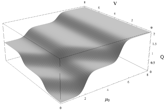
We next compute the steady state charge on the molecule using Eq. (98). As the external bias is increased, different many-body states are populated and the charge on the system increases in steps, similar to the current. This is shown in Fig. 7 for different values of $\mu_{0}$. As the Fermi energy is increased the total system charge at steady state increases and the variation with the bias is decreased. Finally, when the Fermi energy is large enough so that all the many-body states are already populated at $V=0$, the total charge (which is the maximum charge) on the molecule is $2e$ (both system orbitals are occupied) and is independent of the bias.

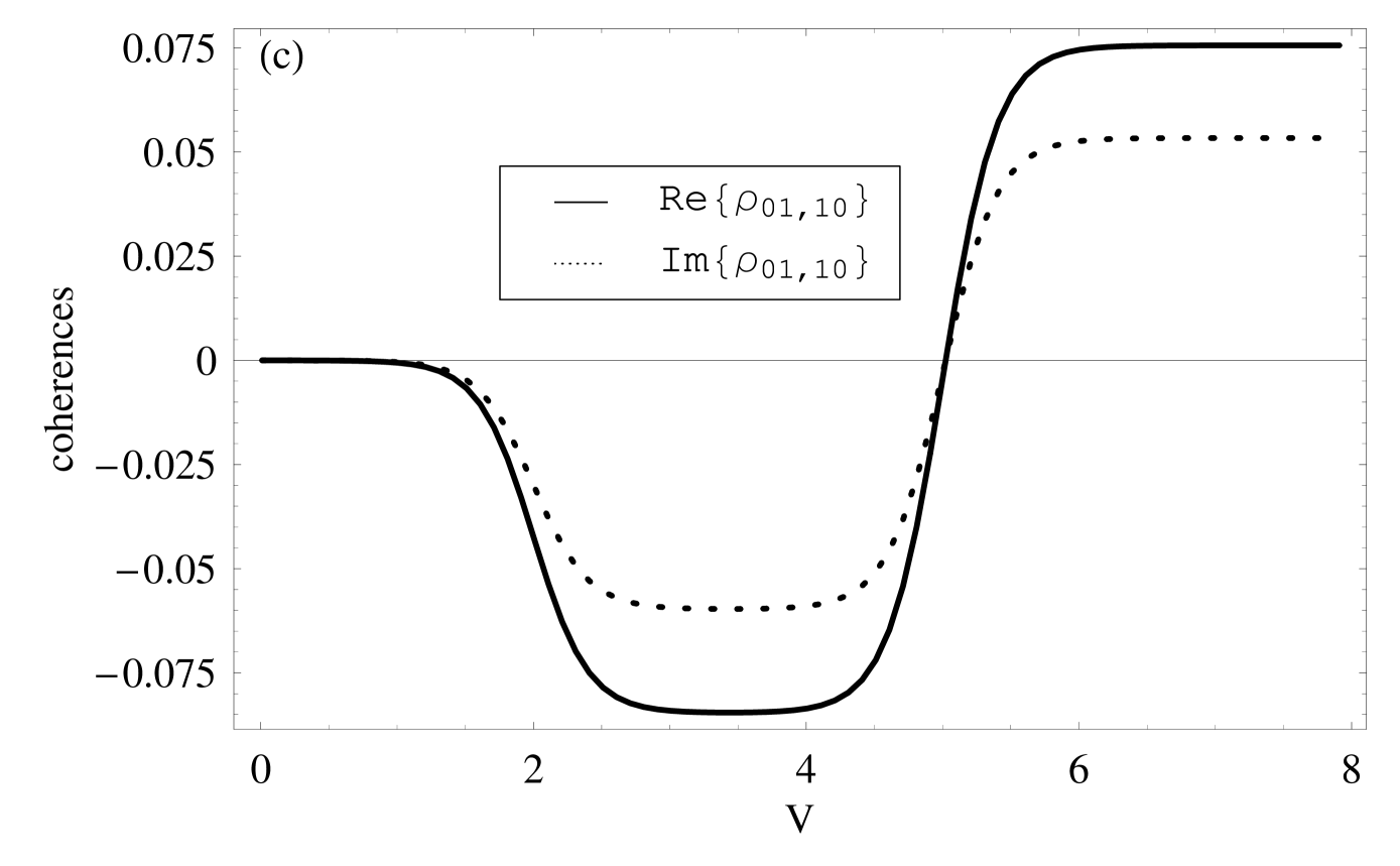
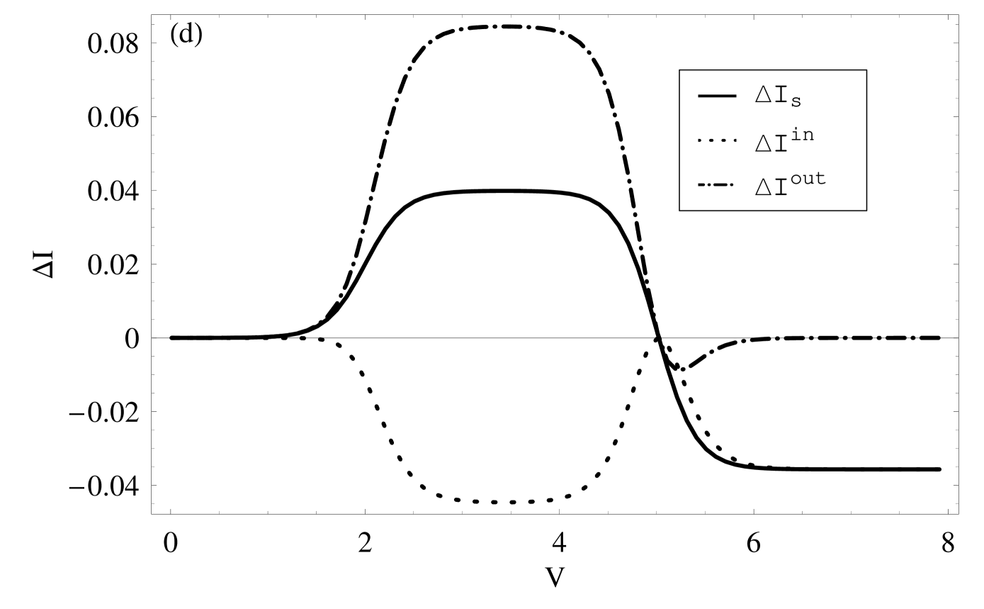
We next study the effect of coherences by solving the QME (33) without invoking the RWA. In this case we need to diagonalize the full $6\times 6$ matrix, $\hat{\cal M}$ and we use Eq. (43) to compute currents numerically. In Figs. 8a and 8b, we present the steady state currents with and without the coherences, respectively. The steady state coherences are shown in Fig. 8c. We note that due to coherences the backward current $I^{out}$ (dash-dot) does not vanish for $eV+\mu_{0}\neq\epsilon_{s}$ and is positive, although it is still maximum and negative at the resonances. This leads to the increase of the total current for smaller bias: coherences produce an effective potential that enhances the potential generated by the chemical potential difference between the leads. In Fig. 8d, we show the change in steady state currents due to coherences at different bias values.

VI Conclusions

The dynamics of a quantum system connected to two metal leads with different chemical potentials is calculated using projection operators which project the total many-body density matrix of the system into the system subspace corresponding to a fixed number of electrons $n$ in Fock space. We derive a set of coupled dynamical equations for the $n$-dependent projected density matrix of the system. When summed over the different possible numbers of electrons $n$ in the system we get a Redfield-like QME for the system many-body density matrix. Since we treat the leads as infinite electron reservoirs, coherences between the leads and the system are not possible. As a result, electron transfer between the leads and the system occurs in an incoherent way. This amounts to eliminating the coherences between system many-body states with different $n$ (FSC) leading to a drastic reduction of the many-body system space. By studying the transient and steady state transport properties of a coupled QD system for arbitrary bias, we showed that coherences between the many body levels corresponding to a same $n$ can affect the transport properties of the quantum system. In the limit of high bias our equation reduces to previously derived QMEs gurvitz ; yan . By invoking the rotating wave approximation, we showed that the populations obey an independent birth and death master equation. In this limit, the QME can be solved analytically for an arbitrary number of orbitals since the system many-body density matrix is a direct product of the individual single-orbital density matrices. Both, in the high bias limit and in the RWA, our QME assumes the Lindblad form. We note that the full QME, Eq. (10), is not in the Lindblad form and may break positivity for strong lead-system couplings. Using the numerical solution of the QME for physically acceptable parameter range, we found that quantum coherences can modify the transport properties of the system.

Appendix A Derivation of the quantum master equation

In order to compute the time dependence of $\rho^{n}(t)$ we start with the Liouville equation for the total density matrix, $\rho_{T}$.

$$\frac{\partial{\tilde{\rho}_{T}}}{\partial t}=-i[\tilde{H}_{T}(t),{\tilde{\rho}_{T}}(t)]$$ (48)

where ${\tilde{\rho}_{T}}(t)$ represents the many-body density matrix and $\tilde{H}_{T}$ is the coupling Hamiltonian, both in the interaction picture.

$$\tilde{\rho}_{T}(t) \equiv e^{iH_{0}t}\rho_{T}(t)e^{-iH_{0}t}$$ (49)

where $H_{0}=H_{s}+H_{L}+H_{R}$ and $\rho_{T}(t)$ is in the Schrodinger picture evolving with the total Hamiltonian, $H$. The interaction picture operators are similarly defined by

$$\tilde{H}_{T}(t) \equiv e^{iH_{0}t}H_{T}e^{-iH_{0}t}.$$ (50)

Substituting $H_{T}$ from Eq. (5) in (48), multiplying by ${\cal P}_{n}$ from both sides, taking a trace over the leads space and using Eq. (9) we obtain the equation of motion for ${\tilde{\rho}}^{n}$.

$$\frac{\partial{\tilde{\rho}}^{n}(t)}{\partial t}=-i\sum_{s\nu}T_{s\nu}\left[A_{s\nu}(t)-B_{s\nu}(t)\right]+h.c.$$ (51)

where

$$A_{s\nu}(t) = e^{i\epsilon_{s\nu}t}\mbox{Tr}_{lead}\left\{c_{s}^{\dagger}c_{\nu}{\cal P}_{n-1}{\tilde{\rho}_{T}}(t){\cal P}_{n}\right\}$$

$$B_{s\nu}(t) = e^{i\epsilon_{s\nu}t}\mbox{Tr}_{lead}\left\{{\cal P}_{n}{\tilde{\rho}_{T}}(t){\cal P}_{n+1}c_{s}^{\dagger}c_{\nu}\right\},$$ (52)

and $\epsilon_{s\nu}=\epsilon_{s}-\epsilon_{\nu}$. In deriving Eq. (51), we have used the relations,

$${\cal P}_{n}c_{s}^{\dagger}c_{\nu}=c_{s}^{\dagger}c_{\nu}{\cal P}_{n-1},~{}~{}~{}~{}~{}~{}{\cal P}_{n}c_{\nu}^{\dagger}c_{s}=c_{\nu}^{\dagger}c_{s}{\cal P}_{n+1}.$$ (53)

Differentiating both sides of Eq. (A) with respect to time and using Eq. (48), we obtain

$$\frac{\partial A_{s\nu}(t)}{\partial t} = i\epsilon_{s\nu}A_{s\nu}(t)-ie^{i\epsilon_{s\nu}t}\sum_{s^{\prime}\nu^{\prime}}e^{-i\epsilon_{s^{\prime}\nu^{\prime}}t}$$ (54)

$$\times \left\{T_{s^{\prime}\nu^{\prime}}^{*}\left[c_{s}^{\dagger}c_{s^{\prime}}\mbox{Tr}_{lead}\left\{c_{\nu}c^{\dagger}_{\nu^{\prime}}{\cal P}_{n}{\tilde{\rho}_{T}}(t){\cal P}_{n}\right\}-c_{s}^{\dagger}\mbox{Tr}_{lead}\left\{c_{\nu}{\cal P}_{n-1}{\tilde{\rho}_{T}}(t){\cal P}_{n-1}c_{\nu^{\prime}}^{\dagger}\right\}c_{s^{\prime}}\right]\right.$$

$$+ \left.T_{s^{\prime}\nu^{\prime}}\left[c_{s}^{\dagger}\mbox{Tr}_{lead}\left\{c_{\nu}{\cal P}_{n-1}{\tilde{\rho}_{T}}(t){\cal P}_{n+1}c_{\nu^{\prime}}\right\}c_{s^{\prime}}^{\dagger}-c_{s}^{\dagger}c_{s^{\prime}}^{\dagger}\mbox{Tr}_{lead}\left\{c_{\nu}c_{\nu^{\prime}}{\cal P}_{n-2}{\tilde{\rho}_{T}}(t){\cal P}_{n}\right\}\right]\right\}$$

$$\frac{\partial B_{s\nu}(t)}{\partial t} = i\epsilon_{s\nu}B_{s\nu}(t)-ie^{i\epsilon_{s\nu}t}\sum_{s^{\prime}\nu^{\prime}}e^{-i\epsilon_{s^{\prime}\nu^{\prime}}t}$$ (55)

$$\times \left\{T_{s^{\prime}\nu^{\prime}}^{*}\left[c_{s^{\prime}}\mbox{Tr}_{lead}\left\{c^{\dagger}_{\nu^{\prime}}{\cal P}_{n+1}{\tilde{\rho}_{T}}(t){\cal P}_{n+1}c_{\nu}\right\}c_{s}^{\dagger}-\mbox{Tr}_{lead}\left\{{\cal P}_{n}{\tilde{\rho}_{T}}(t){\cal P}_{n}c_{\nu^{\prime}}^{\dagger}c_{\nu}\right\}c_{s^{\prime}}c_{s}^{\dagger}\right]\right.$$

$$+ \left.T_{s^{\prime}\nu^{\prime}}\left[\mbox{Tr}_{lead}\left\{{\cal P}_{n}{\tilde{\rho}_{T}}(t){\cal P}_{n+2}c_{\nu^{\prime}}c_{\nu}\right\}c_{s^{\prime}}^{\dagger}c_{s}^{\dagger}-c_{s^{\prime}}^{\dagger}\mbox{Tr}_{lead}\left\{c_{\nu^{\prime}}{\cal P}_{n-1}{\tilde{\rho}_{T}}(t){\cal P}_{n+1}c_{\nu}\right\}c_{s}^{\dagger}\right]\right\}.$$

This hierarchy involves successively higher coherences in Fock space. The first term in the r.h.s. of Eqs. (54) and (55) represents the oscillatory time evolution due to the free molecule Hamiltonian. The other terms represent the evolution due to the coupling with the leads and involve populations and two-electron coherences in the molecule.

We approximate each lead as a free electron gas described by the grand canonical density matrix $\rho_{B}(t)=\rho_{L}\rho_{R}$, where $\rho_{L}$ and $\rho_{R}$ are the density matrices for the left and the right leads with chemical potentials $\mu_{L}$ and $\mu_{R}$, respectively. We assume that the two leads have an infinite capacitance and are not affected by the weak coupling to the system. Both leads are therefore at equilibrium with their respective chemical potentials and the FSC in the leads vanish. This results in the loss of coherences between states with different number of electrons in the molecule and Eqs. (54) and (55) take the form

$$\frac{\partial A_{s\nu}(t)}{\partial t} = i\epsilon_{s\nu}A_{s\nu}(t)-ie^{i\epsilon_{s}t}\sum_{s^{\prime}\nu^{\prime}}e^{-i\epsilon_{s^{\prime}}t}T_{s^{\prime}\nu^{\prime}}^{*}\left[c_{s}^{\dagger}c_{s^{\prime}}{\tilde{\rho}}^{n}(t){\cal C}_{\nu\nu^{\prime}}(t-{t^{\prime}})-c_{s}^{\dagger}{\tilde{\rho}}^{n-1}(t)c_{s^{\prime}}{\cal D}_{\nu\nu^{\prime}}(t-{t^{\prime}})\right]$$ (56)

$$\frac{\partial B_{s\nu}(t)}{\partial t} = i\epsilon_{s\nu}B_{s\nu}(t)-ie^{i\epsilon_{s}t}\sum_{s^{\prime}\nu^{\prime}}e^{-i\epsilon_{s^{\prime}}t}T_{s^{\prime}\nu^{\prime}}^{*}\left[c_{s^{\prime}}{\tilde{\rho}}^{n+1}(t)c_{s}^{\dagger}{\cal C}_{\nu\nu^{\prime}}(t-{t^{\prime}})-{\tilde{\rho}}^{n}(t)c_{s^{\prime}}c_{s}^{\dagger}{\cal D}_{\nu\nu^{\prime}}(t-{t^{\prime}})\right]$$ (57)

where ${\cal C}_{\nu\nu^{\prime}}(t-{t^{\prime}})=\mbox{Tr}_{lead}\left\{c_{\nu}(t)c_{\nu^{\prime}}^{\dagger}({t^{\prime}})\rho_{B}\right\}$ and ${\cal D}_{\nu\nu^{\prime}}(t-{t^{\prime}})=\mbox{Tr}_{lead}\left\{c_{\nu^{\prime}}^{\dagger}({t^{\prime}})c_{\nu}(t)\rho_{B}\right\}$ are the correlation functions for the leads.

The formal solution of Eqs. (56) and (57) is

$$A_{s\nu}(t) = -ie^{i\epsilon_{s}t}\int_{0}^{t}d{t^{\prime}}\sum_{s^{\prime}\nu^{\prime}}e^{-i\epsilon_{s^{\prime}}{t^{\prime}}}T_{s^{\prime}\nu^{\prime}}^{*}\left[c_{s}^{\dagger}c_{s^{\prime}}{\tilde{\rho}}^{n}({t^{\prime}}){\cal C}_{\nu\nu^{\prime}}(t-{t^{\prime}})-c_{s}^{\dagger}{\tilde{\rho}}^{n-1}({t^{\prime}})c_{s^{\prime}}{\cal D}_{\nu\nu^{\prime}}(t-{t^{\prime}})\right]$$ (58)

$$B_{s\nu}(t) = -ie^{i\epsilon_{s}t}\int_{0}^{t}d{t^{\prime}}\sum_{s^{\prime}\nu^{\prime}}e^{-i\epsilon_{s^{\prime}}{t^{\prime}}}T_{s^{\prime}\nu^{\prime}}^{*}\left[c_{s^{\prime}}{\tilde{\rho}}^{n+1}({t^{\prime}})c_{s}^{\dagger}{\cal C}_{\nu\nu^{\prime}}(t-{t^{\prime}})-{\tilde{\rho}}^{n}({t^{\prime}})c_{s^{\prime}}c_{s}^{\dagger}{\cal D}_{\nu\nu^{\prime}}(t-{t^{\prime}})\right]$$ (59)

Since the leads are at equilibrium, their correlation functions are

$${\cal C}_{\nu\nu^{\prime}}(\tau) = \delta_{\nu\nu^{\prime}}(1-f_{\nu})e^{-i\epsilon_{\nu}\tau}$$ (60)

$${\cal D}_{\nu\nu^{\prime}}(\tau) = \delta_{\nu\nu^{\prime}}f_{\nu}e^{-i\epsilon_{\nu}\tau}$$ (61)

where $f_{\nu}=[\mbox{exp}\{\beta(\epsilon_{\nu}-\mu_{\nu})\}+1]^{-1}$ with $\mu_{\nu}=\mu_{L}$ or $\mu_{R}$, $\nu=l$ or $r$.

Substituting Eqs. (58) and (59) in Eq. (51) and making the change of variable, $t-{t^{\prime}}=\tau$, we obtain,

$$\frac{\partial{\tilde{\rho}}^{n}(t)}{\partial t} = \sum_{ss^{\prime}}\int_{0}^{t}d\tau e^{i\epsilon_{ss^{\prime}}t}\left[\alpha_{ss^{\prime}}(\tau)c_{s^{\prime}}(-\tau){\tilde{\rho}}^{n+1}(t-\tau)c_{s}^{\dagger}-\beta_{ss^{\prime}}(\tau){\tilde{\rho}}^{n}(t-\tau)c_{s^{\prime}}(-\tau)c_{s}^{\dagger}\right.$$ (62)

$$- \left.\alpha_{ss^{\prime}}(\tau)c_{s}^{\dagger}c_{s^{\prime}}(-\tau){\tilde{\rho}}^{n}(t-\tau)+\beta_{ss^{\prime}}(\tau)c_{s}^{\dagger}{\tilde{\rho}}^{n-1}(t-\tau)c_{s^{\prime}}(-\tau)\right]+h.c.$$

where $\epsilon_{ss^{\prime}}=\epsilon_{s}-\epsilon_{s^{\prime}}$ and we have used the notation

$$\alpha_{ss^{\prime}}(\tau) = \sum_{\nu\nu^{\prime}}T_{s\nu}T_{s^{\prime}\nu}^{*}{\cal C}_{\nu\nu^{\prime}}(\tau)=\sum_{\nu}T_{s\nu}T_{s^{\prime}\nu}^{*}(1-f_{\nu})e^{-i\epsilon_{\nu}\tau}$$

$$\beta_{ss^{\prime}}(\tau) = \sum_{\nu\nu^{\prime}}T_{s\nu}T_{s^{\prime}\nu}^{*}{\cal D}_{\nu\nu^{\prime}}(\tau)=\sum_{\nu}T_{s\nu}T_{s^{\prime}\nu}^{*}f_{\nu}e^{-i\epsilon_{\nu}\tau}.$$ (63)

Transforming Eq. (62) back to the Schrodinger picture, we get

$$\frac{\partial\rho^{n}(t)}{\partial t} = -i[H_{s},\rho^{n}(t)]+\sum_{ss^{\prime}}\int_{0}^{t}d\tau\left[\alpha_{ss^{\prime}}(\tau)e^{-iH_{0}\tau}c_{s^{\prime}}\rho^{n+1}(t-\tau)e^{iH_{0}\tau}c_{s}^{\dagger}\right.$$ (64)

$$- \left.\alpha_{ss^{\prime}}(\tau)c_{s}^{\dagger}e^{-iH_{0}\tau}c_{s^{\prime}}\rho^{n}(t-\tau)e^{iH_{0}\tau}-\beta_{ss^{\prime}}(\tau)e^{-iH_{0}\tau}\rho^{n}(t-\tau)c_{s^{\prime}}e^{iH_{0}\tau}c_{s}^{\dagger}\right.$$

$$+ \left.\beta_{ss^{\prime}}(\tau)c_{s}^{\dagger}e^{-iH_{0}\tau}\rho^{n-1}(t-\tau)c_{s^{\prime}}e^{iH_{0}\tau}\right]+h.c.$$

We next expand the density matrix $\rho^{n}(t-\tau)$ perturbatively in the coupling with the leads,

$$\rho^{n}(t-\tau) = e^{-iH_{0}(t-\tau)}\rho^{n}e^{iH_{0}(t-\tau)}+{\cal O}(T)$$ (65)

$$= e^{iH_{0}\tau}\rho^{n}(t)e^{-iH_{0}\tau}+{\cal O}(T)$$

where ${\cal O}(T)$ represents terms that depend on the leads-molecule coupling. Substituting Eq. (65) in (64) and keeping terms to second order in the coupling, we get,

$$\frac{\partial\rho^{n}(t)}{\partial t} = -i[H_{s},\rho^{n}(t)]+\sum_{ss^{\prime}}\int_{0}^{t}d\tau\left[\alpha_{ss^{\prime}}(\tau)c_{s^{\prime}}(-\tau)\rho^{n+1}(t)c_{s}^{\dagger}-\beta_{ss^{\prime}}(\tau)\rho^{n}(t)c_{s^{\prime}}(-\tau)c_{s}^{\dagger}\right.$$ (66)

$$- \left.\alpha_{ss^{\prime}}(\tau))c_{s}^{\dagger}c_{s^{\prime}}(-\tau)\rho^{n}(t)+\beta_{ss^{\prime}}(\tau)c_{s}^{\dagger}\rho^{n-1}(t)c_{s^{\prime}}(-\tau)\right]+h.c.$$

where $c_{s}(\tau)=e^{-i\epsilon_{s}\tau}c_{s}$. Making the Markov approximation (assuming that the lead correlation time is short compared to the time evolution of $\rho^{n}$), the time integration in Eq. (66) can be extended to infinity and the equation becomes local in time.

Substituting Eqs. (60) in (66) and carrying out the time integration, we finally obtain Eq. (10). Note that a similar derivation can be done in Liouville space mukamel ; zwanzig by defining the Liouville space projection operator ${\cal C}_{n}$, ${\cal C}_{n}\rho_{T}=\rho^{n}\rho_{B}$.

Appendix B QME in the Local basis

In this section, we recover Gurvitz’s gurvitz results starting from our QME (10) for a QD system. Gurvitz considered a system of two QD connected in series between two leads. We denote the left and right QD by $a$ and $b$ respectively. We therefore need to transform the QME to the local basis representation. Let us define the unitary transformation matrix $U$ which changes the system eigenbasis to local basis (denoted by indices $i,j$, where $i=a,b$ and $j=a,b$). We have $\displaystyle{\sum_{i}}U^{\dagger}_{si}U_{is^{\prime}}=\delta_{ss^{\prime}}$. The transformed Hamiltonian (1) in local basis then reads as

$$H = \sum_{ij}\epsilon_{ij}c_{i}^{\dagger}c_{j}+\sum_{l}\epsilon_{l}c_{l}^{\dagger}c_{l}+\sum_{r}\epsilon_{r}c_{r}^{\dagger}c_{r}+\sum_{i\nu}\left[T_{i\nu}c^{\dagger}_{i}c_{\nu}+T_{i\nu}^{*}c_{\nu}^{\dagger}c_{i}\right]\;,$$ (67)

with

$$c_{s} = \sum_{i}U_{si}^{\dagger}c_{i},~{}~{}~{}~{}c_{s}^{\dagger}=\sum_{i}c_{i}^{\dagger}U_{si},~{}~{}~{}~{}\epsilon_{ss}=\sum_{ij}U^{\dagger}_{si}\epsilon_{ij}U_{js}$$

$$T_{s\nu} = \sum_{i}U^{\dagger}_{si}T_{i\nu},~{}~{}~{}~{}T_{s\nu}^{*}=\sum_{i}U_{si}T_{i\nu}.$$ (68)

Applying the unitary transformation, the QME can be transformed into the local basis set as

$$\frac{\partial\rho^{n}(t)}{\partial t}=-i\sum_{ij}\epsilon_{ij}[c_{i}^{\dagger}c_{j},\rho^{n}(t)] + \sum_{ij}\left[\alpha_{ji}c_{i}\rho^{n+1}(t)c_{j}^{\dagger}-\beta_{ji}\rho^{n}(t)c_{i}c_{j}^{\dagger}\right.$$ (69)

$$- \left.\alpha_{ij}c_{i}^{\dagger}c_{j}\rho^{n}(t)+\beta_{ij}c_{i}^{\dagger}\rho^{n-1}(t)c_{j}+h.c.\right]$$

where

$$\alpha_{ij} = \sum_{ss^{\prime}}U_{is}\alpha_{ss^{\prime}}U_{s^{\prime}j}^{\dagger}$$

$$\beta_{ij} = \sum_{ss^{\prime}}U_{is}\beta_{ss^{\prime}}U_{s^{\prime}j}^{\dagger}.$$ (70)

Thus the QME structure remains the same. Note that even if we assume that the bath correlation function is diagonal in eigenstate, i.e. $\alpha_{ss^{\prime}}$ and $\beta_{ss^{\prime}}$ are diagonal (which is equivalent to the rotating wave approximation, Sec. III), so that the coherences become decoupled from the populations, in local basis however, since $\alpha_{ij}$ and $\beta_{ij}$ are not diagonal [see Eq. (B)], the populations and coherences are still coupled. These coherences in the local basis, which are different from the coherences in eigenspace studied here, were analyzed by Gurvitz $et$ $al$ gurvitz . Our QME (69) can be applied to Gurvitz’s model of two QDs coupled in series, described by the Hamiltonian (1)

$$H_{s} = \sum_{ij}\epsilon_{ij}c^{\dagger}_{i}c_{j}$$

$$H_{L} = \sum_{l}\epsilon_{l}c^{\dagger}_{l}c_{l},~{}~{}~{}~{}~{}H_{R}=\sum_{r}\epsilon_{r}c^{\dagger}_{r}c_{r}$$

$$H_{T} = \sum_{i\nu}\Omega_{\nu}(c^{\dagger}_{\nu}c_{i}+c_{\nu}c^{\dagger}_{i})$$ (71)

where system Hamiltonian $\epsilon_{aa}=\epsilon_{a}$, $\epsilon_{bb}=\epsilon_{b}$ and $\epsilon_{ab}=\epsilon_{ba}=\Omega_{0}$ is the coupling between two dots. In the reduced Liouville space, where FSC are zero, we use the notation $\langle n_{a}n_{b}|\tilde{\rho}|n_{a}^{\prime}n_{b}^{\prime}\rangle=\tilde{\rho}_{n_{a}n_{b},n_{a}^{\prime}n_{b}^{\prime}}$ in the local basis where $n_{a}$$(n_{b})$ is the occupation of QD $a$ and $b$, respectively. The density matrix in the reduced Liouville space is given by the vector $\tilde{\rho}=(\tilde{\rho}_{00,00}\;,\;\tilde{\rho}_{01,01}\;,\;\tilde{\rho}_{10,10}\;,\;\tilde{\rho}_{11,11}\;,\;\tilde{\rho}_{01,10}\;,\;\tilde{\rho}_{10,01})$. Using Eq. (69), the time evolution of elements of the many-body density matrix in the local basis is given by

$$\dot{\tilde{\rho}}=\hat{\tilde{{\cal M}}}\tilde{\rho}\;,$$ (72)

where

$$\hat{\tilde{{\cal M}}}=\left(\begin{array}[]{cccccc}-2\Re(\beta_{aa}+\beta_{bb})&2\Re\alpha_{bb}&2\Re\alpha_{aa}&0&\alpha_{ab}+\alpha_{ba}^{*}&\alpha_{ba}+\alpha_{ab}^{*}\\ 2\Re\beta_{bb}&-2\Re(\alpha_{bb}+\beta_{aa})&0&2\Re\alpha_{aa}&i\Omega_{0}-\alpha_{ba}^{*}+\beta_{ab}&-i\Omega_{0}-\alpha_{ba}-\beta_{ab}^{*}\\ 2\Re\beta_{aa}&0&-2\Re(\alpha_{aa}+\beta_{bb})&2\Re\alpha_{bb}&-i\Omega_{0}-\alpha_{ab}+\beta_{ba}^{*}&i\Omega_{0}-\alpha_{ab}^{*}+\beta_{ba}\\ 0&2\Re\beta_{aa}&2\Re\beta_{bb}&-2\Re(\alpha_{aa}+\alpha_{bb})&-\beta_{ab}-\beta_{ba}^{*}&-\beta_{ab}^{*}-\beta_{ba}\\ \beta_{ba}+\beta_{ab}^{*}&i\Omega_{0}-\alpha_{ab}^{*}+\beta_{ba}&-i\Omega_{0}-\alpha_{ba}+\beta_{ab}^{*}&-\alpha_{ba}-\alpha_{ab}^{*}&-{\cal X}&0\\ \beta_{ab}+\beta_{ba}^{*}&-i\Omega_{0}-\alpha_{ab}+\beta_{ba}^{*}&i\Omega_{0}-\alpha_{ba}^{*}+\beta_{ab}&-\alpha_{ab}-\alpha_{ba}^{*}&0&-{\cal X}^{*}\end{array}\right),$$ (79)

and ${\cal X}=\alpha_{aa}^{*}+\beta_{aa}^{*}+\alpha_{bb}+\beta_{bb}+i(\epsilon_{a}-\epsilon_{b})$. Note that $\alpha_{ij}=\alpha_{ij}^{L}+\alpha_{ij}^{R}$ and $\beta_{ij}=\beta_{ij}^{L}+\beta_{ij}^{R}$. As done in Ref. gurvitz , we assume a large external bias ($\mu_{0}+eV>\epsilon_{a},\epsilon_{b}>\mu_{0}$) so that the Fermi function for left lead is always $1$ (occupied states) and that for the right lead is always zero (unoccupied states). In this limit electrons are always transferred from left to the right lead and the reverse transport vanishes, i.e. $\alpha_{ij}^{L}=\beta_{ij}^{R}=0$. We further assume that the bath correlation functions are real and that the lead’s density of state is a constant (wide-band approximation). Substituting Eqs. (A) in (B), it is easy to show that

$$\alpha_{ij}=2\pi n_{R}T_{i}^{R}{T^{*}}_{j}^{R},~{}~{}~{}~{}~{}~{}~{}\beta_{ij}=2\pi n_{L}T_{i}^{L}{T^{*}}_{j}^{L}.$$ (80)

Since $T_{a}^{R}=T_{b}^{L}=0$, $\alpha_{aa}=\alpha_{ab}$$=\beta_{ab}=$$\beta_{bb}=0$, and $T_{a}=\Omega_{L}$, $T_{b}=\Omega_{R}$, we get

$$\alpha_{bb}=2\pi n_{R}|\Omega_{R}|^{2},~{}~{}~{}~{}~{}~{}~{}~{}~{}~{}\beta_{aa}=2\pi n_{L}|\Omega_{L}|^{2}$$ (81)

which is same as $\Gamma_{L(R)}$ defined in Eq. (3.4) in Ref. gurvitz . The matrix ${\cal\hat{\tilde{M}}}$ then simplifies to

$$\hat{\tilde{{\cal M}}}=\left(\begin{array}[]{cccccc}-2\Re\beta_{aa}&2\Re\alpha_{bb}&0&0&0&0\\ 0&-2\Re(\alpha_{bb}+\beta_{aa})&0&0&i\Omega_{0}&-i\Omega_{0}\\ 2\Re\beta_{aa}&0&0&2\Re\alpha_{bb}&-i\Omega_{0}&i\Omega_{0}\\ 0&2\Re\beta_{aa}&0&-2\Re\alpha_{bb}&0&0\\ 0&i\Omega_{0}&-i\Omega_{0}&0&+i(\epsilon_{a}-\epsilon_{b})-\beta_{aa}^{*}-\alpha_{bb}&0\\ 0&-i\Omega_{0}&i\Omega_{0}&0&0&-i(\epsilon_{a}-\epsilon_{b})-\beta_{aa}-\alpha_{bb}^{*}\end{array}\right)\;.$$ (88)

We note that populations and coherences are coupled together only through the non-diagonal terms in the free (system) Hamiltonian $\Omega_{0}$. The set of Eqs. (72) then can be written explicitly as

$$\frac{\partial\rho_{00}^{n}}{\partial t} = -2\Re\beta_{aa}\rho_{00}^{n}(t)+2\Re\alpha_{bb}\rho_{22}^{n+1}(t)$$ (89)

$$\frac{\partial\rho_{11}^{n}}{\partial t} = i\Omega_{0}(\rho_{12}^{n}(t)-\rho_{21}^{n}(t))+2\Re\beta_{aa}\rho_{00}^{n-1}(t)+2\Re\alpha_{bb}\rho_{33}^{n+1}(t)$$ (90)

$$\frac{\partial\rho_{22}^{n}}{\partial t} = i\Omega_{0}(\rho_{21}^{n}(t)-\rho_{12}^{n}(t))-2\Re(\alpha_{bb}+\beta_{aa})\rho_{22}^{n}(t)$$ (91)

$$\frac{\partial\rho_{33}^{n}}{\partial t} = 2\Re\beta_{aa}\rho_{22}^{n-1}(t)-2\Re\alpha_{bb}\rho_{33}^{n}(t)$$ (92)

$$\frac{\partial\rho_{12}^{n}}{\partial t} = i\epsilon_{ba}\rho_{12}^{n}(t)+i\Omega_{0}(\rho_{11}^{n}(t)-\rho_{22}^{n}(t))-2\Re(\alpha_{aa}+\beta_{aa})\rho_{12}^{n}(t).$$ (93)

The only difference between Eqs.(89)-(93) and Eqs. (4.10a)-(4.10e) of Ref. gurvitz is in the bookkeeping of electrons. In our case $n$ is the number of electrons in the system whether in Ref. gurvitz $n$ is the number of electron collected in the right lead. However, since we are in the large bias limit, the two are directly related and after summing over $n$, so that $\sum_{n}\rho^{n}_{ij}$$=\sum_{n}\rho^{n\pm 1}_{ij}=\rho_{ij}$, Eqs. (89)- (93) become identical to Gurvitz’s equations.

Appendix C RWA Solution for populations and coherences

In the RWA, populations and coherences evolve independently. As discussed in the main text, the population dynamics described by Eq. (33) obey a birth and death master equation. By diagonalizing the $4\times 4$ generator of the population dynamics and using (45) we get

$$\rho_{00,00}(t) = \frac{\alpha_{11}\alpha_{22}}{\beta_{11}\beta_{22}}C_{2}-\frac{\alpha_{22}}{\beta_{22}}C_{3}e^{-2(\alpha_{11}+\beta_{11})t}-\frac{\alpha_{11}}{\beta_{11}}C_{4}e^{-2(\alpha_{22}+\beta_{22})t}+C_{1}e^{-2(\alpha_{11}+\beta_{11}+\alpha_{22}+\beta_{22})t}$$

$$\rho_{11,11}(t) = C_{2}+C_{3}e^{-2(\alpha_{11}+\beta_{11})t}+C_{4}e^{-2(\alpha_{22}+\beta_{22})t}+C_{1}e^{-2(\alpha_{11}+\beta_{11}+\alpha_{22}+\beta_{22})t}$$

$$\rho_{01,01}(t) = \frac{\alpha_{11}}{\beta_{11}}C_{2}-C_{3}e^{-2(\alpha_{11}+\beta_{11})t}+\frac{\alpha_{11}}{\beta_{11}}C_{4}e^{-2(\alpha_{22}+\beta_{22})t}-C_{1}e^{-2(\alpha_{11}+\beta_{11}+\alpha_{22}+\beta_{22})t}$$

$$\rho_{10,10}(t) = \frac{\alpha_{22}}{\beta_{22}}C_{2}+\frac{\alpha_{22}}{\beta_{22}}C_{3}e^{-2(\alpha_{11}+\beta_{11})t}-C_{4}e^{-2(\alpha_{22}+\beta_{22})t}-C_{1}e^{-2(\alpha_{11}+\beta_{11}+\alpha_{22}+\beta_{22})t}$$ (94)

where the coefficients $C_{1}-C_{4}$ are related to the initial density matrix as follows

$$C_{2} = \frac{\beta_{11}\beta_{22}}{D}$$

$$C_{3} = \frac{\alpha_{11}\beta_{22}}{D}\left(\rho_{11,11}(0)+\rho_{10,10}(0)\right)-\frac{\beta_{11}\beta_{22}}{D}\left(\rho_{00,00}(0)+\rho_{01,01}(0)\right)$$

$$C_{4} = \frac{\alpha_{22}\beta_{11}}{D}\left(\rho_{01,01}(0)+\rho_{11,11}(0)\right)-\frac{\beta_{11}\beta_{22}}{D}\left(\rho_{00,00}(0)+\rho_{10,10}(0)\right)$$

$$C_{1} = \frac{1}{D}\left(\beta_{11}\beta_{22}\rho_{00,00}(0)-\alpha_{11}\beta_{22}\rho_{10,10}(0)-\alpha_{22}\beta_{11})\rho_{01,01}(0)+\alpha_{11}\alpha_{22}\rho_{11,11}(0)\right)\;,$$ (95)

where $\rho_{00,00}(0)+\rho_{01,01}(0)+\rho_{10,10}(0)+\rho_{11,11}(0)=1$ and $D=(\alpha_{11}+\beta_{11})(\alpha_{22}+\beta_{22})$.

The time-dependence of coherences is solely determined by the element ${\cal X}$ of matrix $\hat{\cal M}$

$$\rho_{01,10}(t)=\mbox{e}^{-i\epsilon_{12}t}\mbox{e}^{-(\alpha_{11}^{*}+\beta_{11}^{*}+\alpha_{22}+\beta_{22})t}\rho_{01,10}(0).$$ (96)

and $\rho_{10,01}=\rho_{01,10}^{*}$. When the bath correlation functions are real, coherences oscillate with Bohr frequency ($\epsilon_{12}$) of the system.

The steady state populations are given by

$$\rho_{11,11} = \frac{1}{D}\beta_{11}\beta_{22},~{}~{}~{}~{}~{}~{}~{}~{}\rho_{00,00}=\frac{1}{D}\alpha_{11}\alpha_{22}$$

$$\rho_{01,01}^{1} = \frac{1}{D}\alpha_{11}\beta_{22},~{}~{}~{}~{}~{}~{}~{}\rho_{10,10}^{1}=\frac{1}{D}\beta_{11}\alpha_{22}.$$ (97)

Note that steady state coherences are zero. Using Eq. (C) in (41) it is then easy to show that the total steady state charge on the system is

$$Q_{s}=\sum_{s}\frac{\beta_{ss}}{\alpha_{ss}+\beta_{ss}}.$$ (98)

Fig. 1: (a) Lead-system-lead configuration. $a^{+}(a^{-})$ and $b^{+}(b^{-})$ represent the charge transfer processes which change the number of electrons in the system due to interaction with the left (right) lead. (b) Energetics of the junction. $\mu_{L}$ and $\mu_{R}$ are the chemical potentials of the left and right leads. $E_{1}$, $E_{2}$, $E_{3}$ and $E_{4}$ are the energies of the system many-body states.

Fig. 2: The Four many-body states $|n_{1},n_{2}\rangle$ for a model system of two orbitals with occupations $n_{1}$ and $n_{2}$ and energies $\epsilon_{1}$ and $\epsilon_{2}$, respectively. $N=0,1,2$ represents the total number of electrons in the system Fock space. Dashed and Solid lines denote the single-electron and many-electron states, respectively. $E_{1},E_{2},E_{3}$ and $E_{4}$ are the energies of the four many-body states.

Fig. 3: The eigenvalue spectrum (in eV) of the matrix ${\cal M}$ for $V=.1$, $\mu_{0}=0$, $TL_{1}=.01$, $TL_{2}=.02$, $TR_{1}=.03$ and $TR_{2}=.04$. All parameters are in units of $eV$.

Fig. 4: (a) Time evolution of the populations (Eq. C) for $V=2$. Other parameters are same as in Fig. 2. Time is in units of $\hbar/eV$. (b) Time evolution of the real ($\mbox{Re}\rho_{01,10}$) and the imaginary parts ($\mbox{Im}\rho_{01,10}$) of coherences.

Fig. 5: Steady state populations (Eq. C) for $\mu_{0}=0$. The left and right coupling are the same, $TL_{1}=TR_{1}=0.2$ and $T_{L}2=TR_{2}=0.3$. All parameters are in $eV$.

Fig. 6: Current characteristics of the model system using Eqs. (IV) and (47) for parameter of Fig. 4. $I^{in}$: dotted, $I^{out}$: dashed and $I_{s}$: solid curve. Current is in units of $e^{2}V/\hbar$.

Fig. 7: Steady state charge ($Q$) on the system as a function of the applied bias ($V$) and the Fermi energy ($\mu_{0}$).

Fig. 8: (a) Steady state currents obtained by solving Eqs. (43) and (IV) and (b) without coherences, Eq. (47). Comparing to (a), we note that in the absence of coherences, $I^{out}$ is significant only at the resonances and is always negative. (c)The steady state coherences in the system and (d) change in the steady state currents due to coherences. The couplings are $TL_{1}=.4$, $TL_{2}=.7$, $TR_{1}=.4$, $TL_{1}=.2$ and $\mu_{0}=0$ all in units of $eV$.

Figure 1:

Figure 2:

Figure 3:

Figure 4:

Figure 5:

Figure 6:

Figure 7:

Figure 8:

References

• (1) M. A. Reed, C. Zhou, C. J. Muller, T. P. Burgin and J. M. Tour, Science, 278, 252 (1997).
• (2) H. Park, J. Park, A. K. L. Lim, E. H. Anderson, A. P. Alivisatos and P. L. McEuen, Nature 407, 57 (2000).
• (3) T. Dadosh, Y. Gordin, R. Krahne, I. Khivrich, D. Mahalu, V. Frydman, J. Sperling, A. Yacoby, I. Bar-Joseph, Nature 436, 677 (2005).
• (4) M. Avinun-Kalish, M. Heiblum, O. Zarchin, D. Mahalu, and V. Umansky, Nature 436, 529 (2005).
• (5) H. Ohtani, R. J. Wilson, S. Chiang and C. M. Mate, Phys. Rev. Lett 60, 2398 (1988).
• (6) B. C. Stipe, M. A. Rezaei and W. Ho, Science 280, 1732 (1998); S. W. Wu, G. V. Nazin, X. Chen, X. H. Qiu and W. Ho, Phys. Rev. Lett. 93, 236802 (2004); W. Ho, J. Chem. Phys. 117, 11033 (2002).
• (7) A. Nitzan, Ann. Rev. Phys. Chem. 52, 681 (2001).
• (8) A. Nitzan and M. A. Ratner, Nature 300, 1384 (2003). M. Ratner, Nature 435, 575 (2005).
• (9) R. H. M. Smit, Y. Noat, C. Untied, N. D. Lang, M. C. van Hermert and J. M. van Ruitenbeek, Nature 419, 906 (2002).
• (10) W. A. Hofer, A. S. Foster and A. L. Shluger, Rev. Mod. Phys. 75, 1287 (2003).
• (11) P. Sautet, Chem. Rev. 97, 1097 (1997).
• (12) A. Pecchia and A. Di. Carlo, Rep. Prog. Phys. 67, 1497 (2004).
• (13) C. A. Stafford and Ned S. Wingreen, Phys. Rev. Lett. 76, 1916 (1996).
• (14) W. G. van der Wiel, S. De Franceschi, J. M. Elzerman, T. Fujisawa, S. Tarucha and L. P. Kouwenhoven, Rev. Mod. Phys. 75, 1 (2003).
• (15) S. Mukamel, Principles of Nonlinear Optical Spectroscopy, Oxford University Press, New York, 1995.
• (16) C. Cohen-Tannoudji, J. Dupont-Roc, and G. Grynberg, Atom-Photon interactions: Basics Processes and Applications (John Wiley and Sons, Inc., New York, 1992).
• (17) P. Sautet and C. Joachim, Phys. Rev. B 38, 12238 (1988); J. Cerda, M. A. Van Hove, P. Sautet and M. Salmeron, Phys. Rev. B 56, 15885 (1997); P. Sautet and C. Joachim, Chem. Phys. Lett. 185, 23 (1991).
• (18) H. Bruus and K. Flensberg, Many-Body Quantum Theory in Condensed Matter Physics, Oxford University Press, New York, (2006).
• (19) H. Haug and A.-P. Jauho, Quantum Kinetics in Transport and Optics of Semiconductors, Springer, Berlin, 1995.
• (20) C. Caroli, R. Combescot, P. Nozieres and D. S.-James, J. Phys. C 5, 21 (1972); M. Galperin, M. A. Ratner and A. Nitzan, J. Chem. Phys. 121, 11965 (2004); T. Mii, S. G. Tikhodeev and H. Ueba, Phys. Rev. B 68, 205406 (2003); U. Harbola, J. Maddox and S. Mukamel, Phys. Rev. B 73, 205404 (2006).
• (21) S. Datta, Electronic Transport in Mesoscopic Systems, Cambridge University Press, Cambridge, 1997.
• (22) H.-P. Breuer and F. Petruccione The Theory of Open Quantum Systems (Oxford University Press, Oxford, 2002).
• (23) F. Haake, Statistical Treatment of Open Systems, Springer Tracts in Modern Physics, Vol. 66 (1973).
• (24) H. Spohn, Rev. Mod. Phys. 53, 569 (1980).
• (25) C.W. Gardiner and P. Zoller, Quantum Noise (Springer, Berlin, 2000).
• (26) U. Weiss, Quantum Dissipative Systems, 2nd ed. (World Scientific, Singapore, 2000).
• (27) Ph. Brune, C. Bruder, and H. Schoeller, Phys. Rev. B 56, 4730 (1997).
• (28) S. A. Gurvitz, Ya. S. Prager, Phys. Rev. B 53, 15932 (1996).
• (29) J. Rammer, A. L. Shelankov and J. Wabnig, Phys. Rev. B 70, 115327 (2004).
• (30) J. N. Pedersen and A. Wacker, Phys. Rev. B 72, 195330 (2005).
• (31) X. Q. Li, J. Luo, Y. G. Yang, P. Cui and Y. J. Yan, Phys. Rev. B 71, 205304 (2005).
• (32) S. Welack, M. Schreiber and U. Kleinekathofer, J. Chem. Phys. 124, 044712 (2006).
• (33) J. Fransson and M. Rasander, Phys. Rev. B 73, 205333 (2006).
• (34) P. Sautet and C. Joachim, Chem. Phys. Lett. 153, 511 (1988); P. Sautet and C. Joachim, Chem. Phys. 135, 99 (1989); P. Sautet and C. Joachim, Ultramicroscopy 42, 115 (1992).
• (35) S. Mukamel, Phys. Rev. Lett. 42, 168 (1979).
• (36) H. Sprekeler, G. Kiesslich, A. Wacker and E. Schöll, Phys. Rev. B 69, 125328 (2004).
• (37) Since only finite number of electrons can reside in the system, the sum over n𝑛n is restricted. It goes from 00 to an upper cut-off (M𝑀M) which is the number of orbitals in the system. So that ρ(t)=n=0Mρn(t)𝜌𝑡superscriptsubscript𝑛0𝑀superscript𝜌𝑛𝑡\rho(t)=\displaystyle{\sum_{n=0}^{M}}\rho^{n}(t). Note that ρn(t)=0superscript𝜌𝑛𝑡0\rho^{n}(t)=0 for n>M𝑛𝑀n>M, and we can ignore the upper cut-off and simply write, ρ(t)=n=0ρn(t)𝜌𝑡subscript𝑛0superscript𝜌𝑛𝑡\rho(t)=\displaystyle{\sum_{n=0}}\rho^{n}(t). This summation is different than the one used in Refs. gurvitz and yan where one gets an infinite heirarchy and in order to get total many-body density matrix n𝑛n has to be summed from zero to infinity.
• (38) D. Kohen, C. C. Marston, and D. J. Tannor, J. Chem. Phys. 107, 5236 (1997).
• (39) E. Geva, E. Rosenman, and D. Tannor, J. Chem. Phys. 113, 1380 (2000).
• (40) F. Haake and M. Lewenstein, 28, 3606 (1983).
• (41) A. Suàrez, R. Silbey, and I. Oppenheim, J. Chem. Phys. 97, 5101 (1992).
• (42) P. Gaspard and M. Nagaoka, J. Chem. Phys. 111, 5668 (1999).
• (43) C. Bruder and H. Schoeller, Phys. Rev. Lett. 72, 1076 (1994).
• (44) S. A. Gurvitz, D. Mozyrsky and G. P. Berman, Phys. Rev. B 72, 205341 (2005).
• (45) R. Zwanzig, Nonequilibrium Statistical Mechanics, Oxford University Press, New York, 2001.
Fig. 1: (a) Lead-system-lead configuration. a+(a)superscript𝑎superscript𝑎a^{+}(a^{-}) and b+(b)superscript𝑏superscript𝑏b^{+}(b^{-}) represent the charge transfer processes which change the number of electrons in the system due to interaction with the left (right) lead. (b) Energetics of the junction. μLsubscript𝜇𝐿\mu_{L} and μRsubscript𝜇𝑅\mu_{R} are the chemical potentials of the left and right leads. E1subscript𝐸1E_{1}, E2subscript𝐸2E_{2}, E3subscript𝐸3E_{3} and E4subscript𝐸4E_{4} are the energies of the system many-body states.
Fig. 2: The Four many-body states |n1,n2ketsubscript𝑛1subscript𝑛2|n_{1},n_{2}\rangle for a model system of two orbitals with occupations n1subscript𝑛1n_{1} and n2subscript𝑛2n_{2} and energies ϵ1subscriptitalic-ϵ1\epsilon_{1} and ϵ2subscriptitalic-ϵ2\epsilon_{2}, respectively. N=0,1,2𝑁012N=0,1,2 represents the total number of electrons in the system Fock space. Dashed and Solid lines denote the single-electron and many-electron states, respectively. E1,E2,E3subscript𝐸1subscript𝐸2subscript𝐸3E_{1},E_{2},E_{3} and E4subscript𝐸4E_{4} are the energies of the four many-body states.