Weak localization correction to the density of transmission eigenvalues in the presence of magnetic field and spin-orbit coupling for a chaotic quantum dot

Abstract

We calculated the weak localization correction to the density of the transmission eigenvalues in the case of chaotic quantum dots in the framework of Random Matrix Theory including the parametric dependence on the magnetic field and spin-orbit coupling. The result is interpreted in terms of spin singlet and triplet Cooperon modes of conventional diagrammatic perturbation theory. As simple applications, we obtained the weak localization correction to the conductance, the shot noise power and the third cumulant of the distribution of the transmitted charge.

I Introduction

Transport in a two dimensional electron gas is affected by the spin-orbit coupling. The most common signature is the weak (anti)localization. It is a small correction to the conductance due to the interference of time reversed trajectories. The sign of the correction depends on the presence or absence of the spin-orbit scattering. The correction is suppressed if a time reversal symmetry breaking magnetic field is presentmesoreview1 ; SimonsAltshuler ; Hikami ; Bergmann . The spin-orbit term in the Hamiltonian has a form of a non-abelian vector potentialMathurStone . In the case of quantum dots, if the spin-orbit coupling strength is position independent, a gauge transformation can be done, which results in an effective Hamiltonian with reduced spin-orbit coupling, and a rich variety of symmetry classes AF . If the spin-orbit coupling depends on the position the transformation can not be done any moreBCH ; CBF . As a consequence, the accessible symmetry classes are the three standard classes of Dyson, classifying the systems according to the presence or absence of time reversal and spin rotation symmetry.

For quantum dots with chaotic dynamics random matrix theory gives a convenient way to describe the transport properties, provided that the electron transit time $\tau_{\rm erg}$ is much shorter than the other time scales of the problem (mean dwell time $\tau_{\rm dw}$, spin-orbit time $\tau_{\rm so}$, magnetic time $\tau_{\rm B}$, inverse level spacing)RMTQTR . Constructing the appropriate RMT models for the crossover between the symmetry classes, the magnetic field and spin-orbit coupling dependence of the average conductance was calculated in Refs. AF, ; BCH, ; CBF, . The theoretical results are confirmed by numerical simulations Jens and they are in good agreement with the experiments Zum02 ; Zum05 .

If one would like to calculate the averages of other transport properties, such as the shot noise power, higher order cumulants of the distribution of the transmitted charge, or any other linear statistics, the density of transmission eigenvalues is needed RMTQTR . Jalabert et al.JPB gave the weak localization correction to the transmission eigenvalue density for chaotic quantum dots belonging to Dyson’s three symmetry classes. Our work extends this result to the crossover regime between these classes. We present a calculation of the dependence of the weak localization correction to the transmission eigenvalue density on spin-orbit coupling and perpendicular magnetic field. For the sake of simplicity we restrict our attention to symmetric dots, i.e. we assume that the two leads attached to the cavity support the same number of channels $N$, and for technical reasons we consider the case of $N\gg 1$.

In some other sense we complement the work done by Nazarov Nazarov95 , who calculated the crossover behaviour of the weak localization correction to the transmission eigenvalue density for disordered samples in dimensions $d=1,2,3$. Here we give the results for $d=0$ corresponding to a quantum dot.

The study of the transmission eigenvalue density is interesting not only because of the practical implications related to the linear statistics, but it is instructive by itself as well, since it gives a deeper insight to the weak (anti)localization phenomenon. In the cases of Dyson’s symmetry classes the weak localization correction to the transmission eigenvalue density is of the form of Dirac delta peaks at the endpoints of the spectrumJPB . Our analytical, closed-form result shows that these peaks broaden in the crossover regime, but the correction still remains singular. Furthermore, similarly to higher dimensional cases of Ref. Nazarov95, , it is possible to identify the peaks as originating from the singlet and triplet sectors of the Cooperon modes of conventional diagrammatic perturbation theory. Our result also enables us to study the transition from weak localization to weak antilocalization on the level of transmission eigenvalues.

As applications, we calculate the weak localization correction to the conductance, the shot noise power and the third cumulant of the distribution of the transmitted charge. In the case of the conductance we recover the result of Ref. BCH, , giving a verification of our calculations. For the shot noise we find that for the symmetric cavities studied in this paper the weak localization correction is absent in the full crossover regime. The third cumulant of the transmitted charge behaves the opposite way. It is “crossover induced” in the sense that the classical contribution vanishes blanter01 ; nagaev02-2 and the weak localization term is nonzero only in the crossover regime.

The paper is organized as follows. In the next section we specify the systems under consideration and the model applied for the RMT description. We briefly summarize the formal definition and the practical importance of the density of transmission eigenvalues. In Sec. III we present our main result, the weak localization correction to the transmission eigenvalue density, and analyze its behaviour as a function of the degree of time reversal and spin rotation symmetry breaking. In Sec. IV we apply our result to the transport properties above. Finally we conclude in Sec. V.

II Description of the systems and the RMT model

Let us consider a chaotic quantum dot with two leads attached to it. We assume, that the number of propagating modes is the same for both leads. We choose the spin-orbit coupling to depend on the position to avoid the reduction of the coupling strength. The weak magnetic field is perpendicular to the plane of the dot. The assumptions for the spin-orbit coupling and the magnetic field ensure that our system exhibits a crossover between Dyson’s standard symmetry classes.

The transmission eigenvalues are the eigenvalues of the matrix product $t^{\prime}t^{\prime\dagger}$. Denoting the number of modes in a lead with $N$, the transmission matrix $t^{\prime}$, describing the transmission from lead 2 to lead 1, is an $N\times N$ matrix with quaternion elements. It is submatrix of $S$, the $2N\times 2N$ scattering matrix of the system:

$$t^{\prime}=W_{1}SW_{2},$$ (1)

where $W_{1}$ is an $N\times 2N$ matrix defined by $(W_{1})_{ij}=1$ if $i=j$ and $0$ otherwise, $W_{2}$ is a $2N\times N$ matrix with $(W_{2})_{ij}=1$ if $i=j+N$ and $0$ otherwise. The product $t^{\prime}t^{\prime\dagger}$ has $2N$ eigenvalues, where the factor two comes from the quaternion structure of the matrix elements. If the system is time reversal invariant, there are $N$ twofold degenerate levels.

We assume that the system can be described with random matrix theory, i.e. $\tau_{\rm erg}\ll$ $\tau_{\rm dw}$, $\tau_{\rm B}$, $\tau_{\rm so}$, where the magnetic time is related to the flux $\Phi$ through the system as AF ; FrahmPichard

$$\frac{1}{\tau_{\rm B}}=\frac{\kappa}{\tau_{\rm erg}}\left(\frac{\Phi}{\Phi_{0}}\right)^{2},$$

where $\Phi_{0}$ is the flux quantum and $\kappa$ is a numerical factor of order unity.

To give a statistical description of the crossover behaviour of the transmission eigenvalues we need an RMT model for the scattering matrix in the crossover regime. This is provided by the “stub model” WavesRM which was adapted for the system under consideration in Ref. BCH, . In this approach the S matrix is represented as

$$S=PU(1-RU)^{-1}P^{\dagger},$$ (2)

with

$$R=Q^{\dagger}rQ.$$

In the above expression $U$ is an $M\times M$ random unitary symmetric matrix taken from Dyson’s circular orthogonal ensembleRMTQTR (COE) and $r$ is a unitary matrix of size $M-2N$. The $2N\times M$ matrix $P$ and the $(M-2N)\times M$ matrix $Q$ are projection matrices with $P_{ij}=\delta_{i,j}$ and $Q_{ij}=\delta_{i+2N,j}$. The quaternion elements of the matrices $U$, $P$, and $Q$ are all proportional to the $2\times 2$ unit matrix $\openone_{2}$. The matrix $r$ is given by

$$r={\rm e}^{-{i\over M}H^{\prime}},$$ (3)

where $\Delta$ is the mean level spacing of the dot. $H^{\prime}$ is an $(M-2N)$ dimensional quaternion matrix generating the perturbations to the dot Hamiltonian,

$$H^{\prime} = ixX\openone_{2}+ia_{\rm so}(A_{1}\sigma_{x}+A_{2}\sigma_{y}).$$

Here $A_{j}$ ($j=1,2$) and $X$ are real antisymmetric matrices of dimension $M-2N$, with $\mbox{Tr}\,\langle A_{i}A_{j}^{\rm T}\rangle=M^{2}\delta_{ij}$ and $\mbox{Tr}\,\langle XX^{\rm T}\rangle=M^{2}$ and $\sigma_{i}$ are the Pauli matrices. The first term in (LABEL:eq:dH) describes the time reversal symmetry breaking through the magnetic field. The second term, having a symplectic symmetry, corresponds to the Rashba and/or Dresselhaus terms in the case of position dependent spin-orbit couplingtauso . The dimensionless parameters $x$ and $a_{\rm so}$ are related to the corresponding time scales as

$$x^{2}=\frac{2\pi\hbar}{\tau_{\rm B}\Delta},\quad a_{\rm so}^{2}=\frac{2\pi\hbar}{\tau_{\rm so}\Delta}.$$

At the end of the calculation the limit $M\rightarrow\infty$ should be taken.

The density of transmission eigenvalues is defined as

$$\begin{array}[]{ll}\rho(T)&=\left\langle\sum_{i}\delta(T-T_{i})\right\rangle\\ &=-\frac{1}{\pi}\lim_{\epsilon\rightarrow 0^{+}}\ \rm{Im}\left\langle\rm{Tr}\frac{1}{T-t^{\prime}t^{\prime\dagger}+i\epsilon}\right\rangle\end{array},$$ (5)

where the trace is taken over channel and spin indices. Having $\rho(T)$ at hand we can calculate the ensemble average of any linear statistics RMTQTR

$$A=\sum_{i=1}^{2N}a(T_{i}),$$

as

$$\langle A\rangle=\int\rho(T)a(T)dT.$$

Prominent examples for linear statistics are the conductance, the shot noise power, or the cumulants of the distribution of transmitted charge RMTQTR ; BB ; LLY95 . The weak localization correction for the linear statistics can be obtained from the weak localization correction to the transmission eigenvalue density.

III Result and discussion

To find the density of transmission eigenvalues, one has to substitute the scattering matrix (2) into the definition (5) using (1), expand the inverses and calculate the average with the help of the diagrammatic technique of Ref. diagrams, up to subleading order in the small parameter $1/N$. The details of the calculation can be found in Appendix A. The result is

$$\rho(T)=\rho_{0}(T)+\delta\rho(T).$$

With the $O(N)$ contribution

$$\rho_{0}(T)=\left\{\begin{array}[]{ll}\frac{2N}{\pi\sqrt{T(1-T)}}&\textrm{if $0<T<1$}\\ 0&\textrm{otherwise}\\ \end{array}\right.,$$ (6)

we recover the known result of Refs. JPB, ; BarangerMello, ; NazarovR, ; RMTQTR, . The factor of two accounts for the spin, as a consequence of the known fact, that the $O(N)$ term is insensitive to the spin-orbit interaction and the magnetic field.

The main result of our paper is the closed-form, analytical expression for the weak localization correction to the density of transmission eigenvalues,

$$\begin{array}[]{c}\delta\rho(T)=\\ \\ \frac{1}{\pi\sqrt{T(1-T)}}\sum\limits_{n=0,1}(-1)^{n}\left(\frac{\Gamma_{1}(y_{n})}{2}+\frac{\Gamma_{2}(y_{n})-\Gamma_{3}(y_{n})}{4}\right)\end{array}$$ (7)

for $0<T<1$ and $0$ otherwise. The variables $y_{n}$ are $y_{0}=T$ and $y_{1}=1-T$. The expression for $\Gamma_{m}$ is

$$\Gamma_{m}(y)=\frac{\gamma_{m}(\gamma_{m}+2N)}{\gamma_{m}^{2}+4N(\gamma_{m}+N)y},$$

with

$$\gamma_{1}=a_{\rm so}^{2}+x^{2},\quad\gamma_{2}=2a_{\rm so}^{2}+x^{2},\quad\gamma_{3}=x^{2}.$$

Note that $\delta\rho(T)$ is antisymmetric with respect to the point $T=1/2$.

As a verification of (7), we consider the limits of Dyson’s symmetry classes. Labeling them in the usual way with the index $\beta$, they correspond to $x^{2},a_{\rm so}^{2}\ll N$ for $\beta=1$ i.e. systems with time reversal and spin rotation symmetry, $x^{2}\gg N$ for $\beta=2$, that is, systems where the time reversal symmetry is broken by the magnetic field and $x^{2}\ll N\ll a_{\rm so}^{2}$ for $\beta=4$, for time reversal invariant systems without spin rotation symmetry. In these limits expression (7) recovers the known result

$$\delta\rho(T)=2{2-\beta\over 4\beta}\left[\delta(T-0^{+})-\delta(T-1+0^{+})\right]$$ (8)

of Refs. RMTQTR, ; JPB, . The factor of two in (8) is due to the twofold degeneracy of transmission eigenvalues for $\beta=1,4$, mentioned in Sec II.

To get some insight how the weak (anti)localization peaks in (8) emerge, let us have a closer look at $\delta\rho(T)$ as it approaches the different limits. For $\gamma_{m}\ll N$ the expression for $\Gamma_{m}(y)$ is well approximated by a Lorentzian in the variable $\sqrt{y}$,

$$\Gamma_{m}(y)\approx\frac{\gamma_{m}/2N}{(\gamma_{m}/2N)^{2}+(\sqrt{y})^{2}}.$$

In the opposite limit, $\gamma_{m}\gg N$, the functions $\Gamma_{m}$ become independent of $y$. Thus going to $\beta=1$, $\Gamma_{2}$ and $\Gamma_{3}$ cancel, and $\Gamma_{1}$, together with the inverse square root prefactor evolves to the peaks in (8) at the edge of the spectrum. Close to $\beta=2$ the correction vanishes. Notice, that $\Gamma_{3}$ is independent of the spin-orbit coupling parameters. Specially in zero magnetic field it always gives Dirac delta contributions at $T=0$ and at $T=1$. Approaching $\beta=4$, the contributions from $\Gamma_{1}$, $\Gamma_{2}$ disappear, thus the zero magnetic field peaks associated with $\Gamma_{3}$ show up as the weak antilocalization correction.

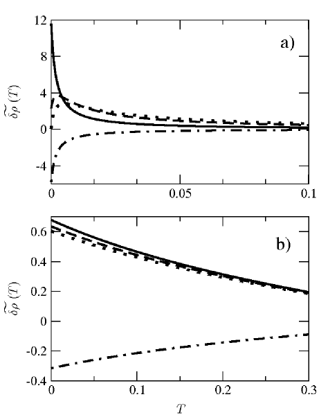
Figure 1: The weak localization weak antilocalization transition for two values of the magnetic field, $x/\sqrt{N}=0.3$ (a) and $x/\sqrt{N}=1.3$ (b). We removed the parameter independent singularities at the endpoints, $\widetilde{\delta\rho\ }(T)=\sqrt{T(1-T)}\delta\rho(T)$. The spin-orbit coupling strength is characterized by $a_{\rm so}/\sqrt{N}=0.0\ ,0.3\ ,0.4\ ,10$ for solid, dashed, dotted and dot-dashed lines respectively.

In the crossover regime the weak localization peaks in (8) broaden, but the correction remains singular at the endpoints. If all the $\gamma_{m}$-s are finite, the singularity is present through a inverse square root factor proportional to the $O(N)$ contribution. The second, nonsingular factor in (7) determines the form of the weak localization correction as the function of the magnetic field and spin-orbit coupling. In the absence of the magnetic field ($\gamma_{3}=0$) this picture is modified by the inclusion of the remanent Dirac delta contribution in place of the $\Gamma_{3}$ term. On Fig. 1 we illustrated the transition from weak localization to weak antilocalization for two values of the magnetic field. The relevant regions are close to the endpoints, where the peaks of the pure symmetry cases (8) are located. Due to the antisymmetry of $\delta\rho(T)$ we plotted only the part around $T=0$.

The presence of spin-orbit coupling dependent and spin-orbit coupling independent contributions is analogous to the case of higher dimensional systems studied by Nazarov Nazarov95 , where they correspond to contributions coming from spin-triplet and spin-singlet Cooperon modes. The situation is very similar in our case. The basic building block of the diagrammatic expansion for $\delta\rho(T)$ is the combination ${\mathcal{T}}C{\mathcal{T}}$, with $\mathcal{T}=\openone_{2}\otimes\sigma_{2}\$ and

$$C^{-1}=M\openone_{2}\otimes\openone_{2}-\mbox{Tr}\,R\otimes\overline{R},$$

where $\overline{()}$ denotes quaternion complex conjugation and the tensor product is defined with a backwards multiplication:

$$(\sigma_{i}\otimes\sigma_{j})(\sigma_{i^{\prime}}\otimes\sigma_{j^{\prime}})=(\sigma_{i}\sigma_{i^{\prime}})\otimes(\sigma_{j^{\prime}}\sigma_{j}).$$ (9)

The trace in the second term is understood as

$$\left(\mbox{Tr}\,R\otimes\overline{R}\right)_{\alpha\beta,\gamma\delta}=R_{ij,\alpha\beta}\overline{R}_{ji,\gamma\delta},$$

where latin letters are channel indices, Greek letters refer to spin space and summation over repeated indices is implied. The very same structure emerges in the work of Brouwer et. al. BCH , where the authors identify $C$ as the equivalent of the Cooperon in the conventional diagrammatic perturbation theory. In the limit $M\rightarrow\infty$ it becomes:

$$C^{-1}=2(N+x^{2}+a_{\rm so}^{2})(\openone_{2}\otimes\openone_{2})-a_{\rm so}^{2}(\sigma_{x}\otimes\sigma_{x}+\sigma_{y}\otimes\sigma_{y}).$$ (10)

If according to the multiplication rule (9) we define the action of a matrix on a vector as $(Av)_{\alpha\beta}=A_{\alpha\rho,\sigma\beta}v_{\rho\sigma}$, the spin-singlet and spin-triplet basis turns out to be the eigenbasis of the matrix ${\mathcal{T}}C{\mathcal{T}}$ with eigenvalues

$$\lambda^{-1}_{00}=2(N+\gamma_{3}),\ \lambda^{-1}_{1\pm 1}=2(N+\gamma_{1}),\ \lambda^{-1}_{10}=2(N+\gamma_{2}).$$

As in Ref. Nazarov95, , only the triplet eigenvalues depend on the spin-orbit coupling strength. The correction (7) can be expressed as

$$\begin{array}[]{c}\delta\rho(T)=\\ \\ \frac{1}{4\pi\sqrt{T(1-T)}}\sum\limits_{n=0,1}(-1)^{n}\left(\sum\limits_{m=-1}^{1}\Gamma(\lambda_{1m},y_{n})-\Gamma(\lambda_{00},y_{n})\right),\end{array}$$ (11)

where the function $\Gamma$ is

$$\Gamma(\lambda,y)=\frac{1-4N^{2}\lambda^{2}}{(1-2N\lambda)^{2}+8N\lambda y}.$$

The appearance of the spin-orbit coupling independent term is because of the decoupling of the singlet and triplet sectors of ${\mathcal{T}}C{\mathcal{T}}$. Going back to the discussion of the weak localization - weak antilocalization transition with (11) in mind, we find that the weak localization peak is due to the triplet terms with eigenvalue $\lambda_{1\pm 1}$, and the weak antilocalization peak comes from the singlet contribution.

An other property of the higher dimensional cases that persists also for quantum dots is the breakdown of the perturbation theory for small magnetic fields near $T=0,1$. More precisely, for fields $x^{2}\lesssim 1$ the applicability condition $\delta\rho\ll\rho$ of the perturbation theory is violated in an interval of order $O(x/N^{2})$ from the endpoints of the spectrum. The conclusion is the same as in Ref. Nazarov95, , namely, at small fluxes, for obtaining the detailed behaviour of the density near $T=0,1$ one has to treat the problem in a nonperturbative way.

IV Applications

Having obtained the $\delta\rho(T)$, let us see some applications. In the following we assume zero temperature. First we compute the conductance. We find

$$\begin{array}[]{ll}G&=\frac{e^{2}}{h}\int_{0}^{1}dT(\rho_{0}(T)+\delta\rho(T))T\\ &=\frac{e^{2}}{h}N\left[1-\left(\frac{1}{2(\gamma_{1}+N)}+\frac{1}{4(\gamma_{2}+N)}-\frac{1}{4(\gamma_{3}+N)}\right)\right],\end{array}$$ (12)

where the second term represents the weak localization correction. It is another verification of (7), as we recover the corresponding result of Brouwer et. al. in Ref. BCH, . Note that the correction is of the form $\delta G\propto\lambda_{00}-\sum_{m=-1}^{1}\lambda_{1m}$ (Ref. Hikami, ; AF, ).

As a second application we consider the shot noise power. We get

$$P=\frac{2e^{3}V}{h}\int_{0}^{1}dT(\rho_{0}(T)+\delta\rho(T))T(1-T)=\frac{2e^{3}V}{h}\frac{N}{4},$$

that is, the $O(1)$ contribution from $\delta\rho(T)$ is absent. In the case of pure symmetry classes it is a known result, that the weak localization correction to the shot noise power vanishes if the number of modes is the same in both leads JPB ; RMTQTR . It was shown in Ref. Braun, that this persists to the case of a $\beta=1\rightarrow 2$ transition too. Our result allows us to extend this prediction to the more general crossover interpolating between all of Dyson’s symmetry classes. The reason behind the absence of the $O(1)$ contribution is that $T(1-T)$ is symmetric with respect to the point $T=1/2$ and it is integrated with the antisymmetric density function $\delta\rho(T)$.

To see an example, where the weak localization correction is absent in the limit of pure symmetry classes, but not in the crossover regime, let us take the third cumulant of the distribution of the transmitted charge. It is the opposite of the shot noise in the sense, that for cavities with leads supporting the same number of channels the $O(N)$ term vanishes blanter01 ; nagaev02-2 , thus the leading order of this quantity is determined by $\delta\rho$. The third cumulant is proportional to

$$f_{3}=\int_{0}^{1}dT(\rho_{0}(T)+\delta\rho(T))T(1-T)(1-2T).$$

The weak localization correction trivially vanishes in the pure symmetry case because of the factor $T(1-T)$ and the Dirac delta functions in (8). In the crossover regime we find

$$f_{3}=N\left(\frac{\gamma_{1}(\gamma_{1}+2N)}{16(\gamma_{1}+N)^{3}}+\frac{\gamma_{2}(\gamma_{2}+2N)}{32(\gamma_{2}+N)^{3}}-\frac{\gamma_{3}(\gamma_{3}+2N)}{32(\gamma_{3}+N)^{3}}\right),$$

that is, the (ensemble average of the) third cumulant is “crossover induced” for a symmetric cavity.

V Conclusions

We investigated the crossover behaviour of the weak localization correction to the density of the transmission eigenvalues between Dyson’s three symmetry classes $\beta=1,2,4$ for a case of a chaotic cavity with symmetric leads. Using the stub model approach for the RMT description, with the help of the diagrammatic method of Brouwer and Beenakker diagrams , we carried out a subleading order calculation in the small parameter $1/N$. Our main finding is a closed-form, analytical expression for the correction.

We studied the weak localization - weak antilocalization transition in detail. We found that the weak (anti)localization peaks (8) of the case of pure symmetry classes broaden in the crossover regime, but the correction still remains singular at the endpoint of the spectrum. With our result (7) at hand, we gave a quantitative description of the broadening and the crossover from localization to antilocalization as the function of the magnetic field and spin-orbit coupling.

We compared our results to the known cases of higher dimensionalities, and found strong similarities. First, our result also splits into spin-singlet and spin-triplet parts, with only the triplet contribution depending on the spin-orbit coupling. In the limits of pure symmetry classes, the weak localization peak comes from the triplet contribution, while the antilocalization peak is due to the singlet part. Second, we also find that for small magnetic fields, the perturbation theory fails to describe the details of the density near the endpoints of the transmission eigenvalue spectrum.

We applied our results to the conductance, the shot noise power and the third cumulant of the distribution of the transmitted charge. The conductance served as a test for our calculations, we recovered the result of Ref. BCH, obtained in the framework of the same model. For the shot noise power we found that the weak localization correction is absent in the full crossover, due to the symmetry of the transmission eigenvalue density. For the third cumulant we found opposite behaviour. It is crossover induced: the $O(N)$ term is absent, and the $O(1)$ contribution is nonzero only in the crossover regime.

Further directions of research could be to apply our result to obtain the weak localization correction to the full statistics of the transmitted charge. Another possibility would be to extend our calculations to the case of cavities with asymmetric leads. In that case, differently from the present results, we expect a nontrivial magnetic field and spin-orbit coupling dependence also for the shot noise power.

Appendix A Details of the calculation

In this appendix we give the details of the derivation of our main result (7). We adapt a procedure of Brouwer and Beenakkerdiagrams that removes the nested geometric series in (5), appearing due to the inverse in the expression (2) for the S matrix. The price for this is the introduction of more complicated matrix structures.

Let us introduce the $2M\times 2M$ matrices

$$\begin{array}[]{c}\begin{array}[]{lll}{\bf S}=\left(\begin{array}[]{cc}S&0\\ 0&S^{\dagger}\end{array}\right),&{\bf C}=\left(\begin{array}[]{cc}0&C_{2}\\ C_{1}&0\end{array}\right),&{\bf U}=\left(\begin{array}[]{cc}U&0\\ 0&U^{\dagger}\end{array}\right),\end{array}\\ \\ \begin{array}[]{ll}{\bf F}(z)=\left(\begin{array}[]{cc}0&F^{\prime}(z)\\ F(z)&0\end{array}\right),&{\bf R}=\left(\begin{array}[]{cc}R&0\\ 0&R^{\dagger}\end{array}\right),\end{array}\end{array}$$ (13)

where for $S$ we use the representation (2) with $P$ being $M\times M$ matrix

$$P_{ij}=1\textrm{ if }i=j\leq 2N\textrm{ and }0\textrm{ otherwise,}$$

and the $M\times M$ matrices $C_{1}$ and $C_{2}$ are

$$(C_{1})_{ij} = 1\textrm{ if }i=j\leq N\textrm{ and }0\textrm{ otherwise}$$

$$C_{2} = P-C_{1}.$$

The Green functions $F_{1}(z)$ and $F_{2}(z)$ are defined as

$$F(z) =C_{1}(z-SC_{2}S^{\dagger}C_{1})^{-1},$$ (14a)

$$F^{\prime}(z) =C_{2}(z-S^{\dagger}C_{1}SC_{2})^{-1}.$$ (14b)

The density of transmission eigenvalues can be obtained from $F(z)$ as

$$\rho(T)=-\pi^{-1}\lim_{\epsilon\rightarrow 0^{+}}\ \mbox{Im}\,\mbox{Tr}\,\langle F(T+i\epsilon)\rangle.$$ (15)

The matrix Green function ${\bf F}(z)$ can be expressed as

$$\begin{array}[]{c}{\bf F}(z)=\\ \\ (2z)^{-1}\sum_{\pm}\left({\bf C}\pm{\bf C}\left[1-{\bf U}({\bf R}\pm{\bf C}z^{-1/2})\right]^{-1}{\bf U}{\bf C}z^{-1/2}\right)\\ \\ =(2z)^{-1}\sum_{\pm}\left[{\bf C}\pm{\bf A}_{\pm}({\bf F}_{\pm}-{\bf X}_{\pm}){\bf B}_{\pm}\right],\end{array}$$ (16)

with ${\bf X}_{\pm}={\bf R}\pm{\bf C}z^{-1/2}$ and ${\bf F}_{\pm}={\bf X}_{\pm}(1-{\bf U}{\bf X}_{\pm})^{-1}$. We defined ${\bf A}_{\pm}$ and ${\bf B}_{\pm}$ such that ${\bf A}_{\pm}{\bf X}_{\pm}={\bf C}$, ${\bf X}_{\pm}{\bf B}_{\pm}={\bf C}z^{-1/2}$.

To get the ensemble average of ${\bf F}$, one has to calculate the COE average of ${\bf F}_{\pm}$. In the following ${\bf F}_{\pm}$ refers to this unitary average. It is related to the self energy ${\bf\Sigma}_{\pm}$ through the Dyson equation

$${\bf F}_{\pm}={\bf X}_{\pm}\left(1+{\bf\Sigma}_{\pm}{\bf F}_{\pm}\right),\ \$$ (17)

We can express $\langle{\bf F}\rangle$ directly through ${\bf\Sigma}_{\pm}$ as

$$\langle{\bf F}\rangle=(2z)^{-1}\sum_{\pm}\left({\bf C}\pm{\bf C}\left\langle(1-{\bf\Sigma}_{\pm}{\bf X}_{\pm})^{-1}{\bf\Sigma}_{\pm}\right\rangle{\bf C}z^{-1/2}\right)$$ (18)

First we calculate ${\bf F}_{\pm}$ to leading order in $\frac{1}{N}$. To this order we have to consider the planar diagrams only. Denoting the resulting series as ${\bf F}^{(0)}_{\pm}$, for the self energy we find

$${\bf\Sigma}^{(0)}_{\pm}=\sum_{n=1}^{\infty}W_{n}\left({\cal P}{\bf F}^{(0)}_{\pm}\right)^{2n-1},$$ (19)

where the coefficients $W_{n}$ are given as diagrams

$$W_{n}={1\over n}N^{1-2n}(-1)^{n-1}{2n-2\choose n-1}.$$

The operator ${\cal P}$ acts on a $2M\times 2M$ matrix ${\bf A}$ as

$${\bf A}=\left(\begin{array}[]{cc}A_{11}&A_{12}\\ A_{21}&A_{22}\end{array}\right),\ \ {\cal P}{\bf A}=\left(\begin{array}[]{cc}0&\mbox{tr}\,A_{12}\\ \mbox{tr}\,A_{21}&0\end{array}\right).$$

With the help of the generating function

$$h(z)=\sum_{n=1}^{\infty}W_{n}z^{n-1}={1\over 2z}\left(\sqrt{M^{2}+4z}-M\right)$$

we can write equation (19) as

$$\begin{array}[]{c}{\bf\Sigma}^{(0)}_{\pm}=\\ \\ \left({\cal P}{\bf X}_{\pm}(1-{\bf\Sigma}^{(0)}_{\pm}{\bf X}_{\pm})^{-1}\right)\,h\left(\left({\cal P}{\bf X}_{\pm}(1-{\bf\Sigma}^{(0)}_{\pm}{\bf X}_{\pm})^{-1}\right)^{2}\right).\end{array}$$

The solution is

$${\bf\Sigma}_{\pm}^{(0)}=\pm\left(\sqrt{z}-\sqrt{z-1}\right)\left(\begin{array}[]{cc}0&1\\ 1&0\end{array}\right).$$ (20)

From (20) it follows that

$$\mathrm{Tr}F_{0}(z)=\mathrm{Tr}F_{0}^{\prime}(z)=\frac{2N}{\sqrt{z(z-1)}},$$

from which we get the well known result (6) for the density of transmission eigenvalues.

In accounting for the weak localization correction let us write the self energy as

$${\bf\Sigma}_{\pm}={\bf\Sigma}_{\pm}^{(0)}+\delta{\bf\Sigma}_{\pm}.$$ (21)

It follows from (18), that ${\bf F}$ splits up too,

$${\bf F}={\bf F}^{(0)}+\delta{\bf F},$$

with $\delta{\bf F}$ containing the weak localization correction to the Green functions (14) in its off-diagonal blocks. Up to first order in $\delta{\bf\Sigma}_{\pm}$, after a little algebra we get

$$\delta{\bf F}=\frac{1}{2}\left(\frac{1}{z}-\frac{1}{z-1}\right)\sum_{\pm}{\mp}\sqrt{z}\ {\bf C}\ \delta{\bf\Sigma}_{\pm}{\bf C}.$$ (22)

The contributions to the self energy correction $\delta{\bf\Sigma}_{\pm}$ come from the $O(\frac{N^{\alpha}}{M^{\alpha+1}})$ terms in the large-$M$ expansion of ${\bf\Sigma}_{\pm}$. These can be sorted as

$$\delta{\bf\Sigma}_{\pm}=\delta{\bf\Sigma}^{(e)}_{\pm}+\sum_{n=1}^{\infty}W_{n}\delta\left({\cal P}{\bf F}_{\pm}\right)^{2n-1}.$$ (23)

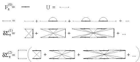
Figure 2: Diagrams contributing to the explicit part $\delta{\bf\Sigma}^{(e)}_{\pm}$ of the weak localization correction to the self energy.

The first term consists of diagrams with the outermost $U$-cycle being non-planar (see Fig. 2), and a term due to the sub-leading order in the large-$M$ expansion of the cumulant coefficients

$$\delta{\bf\Sigma}^{(e)}_{\pm}=\delta{\bf\Sigma}^{(1)}_{\pm}+\delta{\bf\Sigma}^{(2)}_{\pm}+\underbrace{\sum_{n=1}^{\infty}\delta W_{n}\left({\cal P}{\bf F}^{(0)}_{\pm}\right)^{2n-1}}_{\delta{\bf\Sigma}^{(\delta W)}_{\pm}},$$ (24)

with $\delta W_{n}=-\frac{(-4)^{n-1}}{M^{2n}}$. Evaluating the diagrams of Fig. 2 for $\delta{\bf\Sigma}^{(1)}_{\pm}$ we find

$$\begin{array}[]{c}\delta{\bf\Sigma}^{(1)}_{\pm}=\\ \\ \left(\begin{array}[]{cc}aE_{\alpha\sigma,\alpha^{\prime}\sigma^{\prime}}R^{*}_{\sigma^{\prime}\sigma}&bG_{\alpha\sigma,\alpha^{\prime}\sigma^{\prime}}\left(R^{\dagger}R+2C_{2}\right)_{\sigma^{\prime}\sigma}\\ bG_{\alpha\sigma,\alpha^{\prime}\sigma^{\prime}}\left(R^{\dagger}R+2C_{1}\right)_{\sigma^{\prime}\sigma}&aE_{\alpha\sigma,\alpha^{\prime}\sigma^{\prime}}R^{T}_{\sigma^{\prime}\sigma}\\ \end{array}\right)\end{array}$$ (25)

where $()^{*}$ denotes the complex conjugate, Greek indices refer to spin space and we assumed summation for repeated indices. Furthermore

$$a=\frac{\sqrt{z}+\sqrt{z-1}}{2\sqrt{z-1}},\quad b=\pm\frac{1}{2\sqrt{z-1}},$$

$$E=-2Nb^{2}\ \mathcal{T}\Pi\mathcal{T},\quad G=a^{2}\ \mathcal{T}\ C^{-1}\Pi\ \mathcal{T},$$ (26)

with

$$\Pi=\left(a^{4}C^{-2}-(2Nb^{2})^{2}\right)^{-1}.$$

The matrices $\mathcal{T}$ and $C$ are defined as in Sec. III.

The second term $\delta{\bf\Sigma}^{(2)}_{\pm}$ is

$$\delta{\bf\Sigma}^{(2)}_{\pm}=\left((s_{1}+s_{2})Q_{11}+2s_{1}Q_{12}\right)_{\alpha\sigma,\alpha^{\prime}\sigma}\left(\begin{array}[]{cc}0&1\\ 1&0\end{array}\right),$$ (27)

where

$$\begin{array}[]{l}Q=M\left(\begin{array}[]{cc}a^{2}G+b^{2}E&a^{2}E+b^{2}G\\ a^{2}E+b^{2}G&a^{2}G+b^{2}E\end{array}\right)\times\\ \\ \left(\begin{array}[]{cc}a^{2}{\rm Tr}R\otimes R^{*}&b^{2}(M-2N)\\ b^{2}(M-2N)&a^{2}{\rm Tr}R\otimes R^{*},\end{array}\right)\end{array}$$

where the trace is defined as in Sec. III and

$$s_{1}=-\frac{b}{M^{2}}\left(\frac{z-1}{z}\right)^{3/2}\quad s_{2}=\left(1-4z\frac{b^{2}}{a^{2}}\right)s_{1}.$$

Doing the summation in the third term in (24) we get

$$\delta{\bf\Sigma}^{(\delta W)}_{\pm}=-\frac{b}{M}\frac{z-1}{z}\left(\begin{array}[]{cc}0&1\\ 1&0\end{array}\right).$$ (28)

The second term in (23) contains sub-leading order diagrams, that have planar outermost $U$-cycles. Up to first order in $\delta{\bf\Sigma}_{\pm}$

$$\begin{array}[]{c}\delta\left({\cal P}{\bf F}_{\pm}\right)^{2n-1}=\\ \\ \left({\cal P}{\bf F}^{(0)}_{\pm}+{\cal P}\left({\bf F}^{(0)}_{\pm}\delta{\bf\Sigma}_{\pm}{\bf F}^{(0)}_{\pm}\right)\right)^{2n-1}-\left({\cal P}{\bf F}^{(0)}_{\pm}\right)^{2n-1}.\end{array}$$

Putting everything together we see, that (23) is a (linear) self-consistency equation for $\delta{\bf\Sigma}_{\pm}$, which can be solved straightforwardly, if from (22) we notice, that for the transmission eigenvalue density it is enough to get ${\rm Tr}_{2}\ \delta{\bf\Sigma}_{\pm}$, where we denoted the spin-trace as ${\rm Tr}_{2}$. Substituting the solution in (22) in the lower left block we get the weak localization correction to $F(z)$, from which using (15) we arrive to the result (7).

References

- (1) C. W. J. Beenakker and H. van Houten, Solid State Phys. 44, 1 (1991).
- (2) B. L. Altshuler and B. D. Simons in Mesoscopic Quantum Physics, edited by E. Akkermans, G. Montambaux, J.-L. Pichard, and J. Zinn-Justin (North Holland, Amsterdam, 1995).
- (3) S. Hikami, A. I. Larkin, and Y. Nagaoka, Prog. Theor. Phys. 63, 707 (1980).
- (4) G. Bergmann, Phys. Rep. 107, 1 (1984).
- (5) H. Mathur and A. D. Stone, Phys. Rev. Lett. 68, 2964 (1992).
- (6) I. L. Aleiner and V. I. Fal’ko, Phys. Rev. Lett. 87, 256801 (2001); 89, 079902(E) (2002).
- (7) P. W. Brouwer, J. N. H. J. Cremers, and B. I. Halperin, Phys. Rev. B 65, 081302 (2002).
- (8) J.H. Cremers, P.W. Brouwer, and V.I. Falko, Phys. Rev. B 68, 125329 (2003)
- (9) C. W. J. Beenakker, Rev. Mod. Phys. 69, 731 (1997).
- (10) J. H. Bardarson, J. Tworzydlo and C. W. J. Beenakker, Phys. Rev. B. 72, 235305 (2005).
- (11) D. M. Zumbühl, J. B. Miller, C. M. Marcus, K. Campman, and A. C. Gossard, Phys. Rev. Lett. 89, 276803 (2002).
- (12) D. M. Zumbühl, J. B. Miller, D. Goldhaber-Gordon, C. M. Marcus, J. S. Harris, K. Campman, and A. C. Gossard, Phys. Rev. B. 72, 081305 (2005) .
- (13) R. A. Jalabert, J.-L. Pichard, and C. W. J. Beenakker, Europhys. Lett. 27, 255 (1994).
- (14) Y. V. Nazarov, Phys. Rev. B 52, 4720 (1995).
- (15) Ya. M. Blanter, H. Schomerus and C. W. J. Beenakker, 2001 Physica E 11 1
- (16) K. E. Nagaev,P. Samuelsson and S. Pilgram, 2002 Phys. Rev. B 66 195318
- (17) K. M. Frahm and J.-L. Pichard, J. Phys. (France) I 5, 847 (1995).
- (18) P. W. Brouwer, K. M. Frahm, and C. W. J. Beenakker, Waves in Random Media 9, 91 (1999) 37, 4904 (1996)
- (19) Regarding the relation between the spin orbit time and the Rashba/Dresselhaus parameters we refer to Refs. BCH, ; CBF, .
- (20) Ya. M. Blanter and M. Büttiker, Physics Reports 336, 1-166 (2000).
- (21) H. Lee, L. S. Levitov, and A. Yu. Yakovets, Phys. Rev. B 51 (1995) 4079.
- (22) P. W. Brouwer and C. W. J. Beenakker, J. Math. Phys.
- (23) H. U. Baranger and P. A. Mello, Phys. Rev. Lett. 73, 142 (1994).
- (24) Yu. V. Nazarov, in Quantum Dynamics of Submicron Structures, edited by H. A. Cerdeira, B. Kramer, and G. Schön, NATO ASI Series E291 (Kluwer, Dordrecht, 1995).
- (25) P. Braun, S. Heusler, S. Müller and F. Haake, J. Phys. A: Math. Gen. 39, L159-L165 (2006).