Electronic transmission in a model quantum wire with side coupled quasiperiodic chains: Fano resonance and related issues

Abstract

We present exact results for the transmission coefficient of a linear lattice at one or more sites of which we attach a Fibonacci quasiperiodic chain. Two cases have been discussed, viz, when a single quasiperiodic chain is coupled to a site of the host lattice and, when more than one dangling chains are grafted periodically along the backbone. Our interest is to observe the effect of increasing the size of the attached quasiperiodic chain on the transmission profile of the model wire. We find clear signature that, with a side coupled semi-infinite Fibonacci chain, the Cantor set structure of its energy spectrum should generate interesting multifractal character in the transmission spectrum of the host lattice. This gives us an opportunity to control the conductance of such systems and to devise novel switching mechanism that can act over arbitrarily small scales of energy. The Fano profiles in resonance are observed at various intervals of energy as well. Moreover, an increase in the number of such dangling chains may lead to the design of a kind of spin filters. This aspect is discussed.

I Introduction

Electronic properties of simple one and quasi-one dimensional model systems have been studied with keen interest over the past few years. This is mainly due to the success of nanofabrication techniques in producing extremely small quantum objects characterised by discrete energy levels and novel transport properties, which can be examined in a controllable way gold98 -shang01 . Precision instruments such as the scanning tunnel microscope (STM) can now be used to build low dimensional nanostructures with tailor made geometries, such as one dimensional wires and confined two dimensional structures sund91 -gam00 . The tip of an STM can act as tweezers and can practically ‘place’ individual atoms on a substrate. Thus, simple low dimensional model quantum systems are now closer to reality.

In recent times, there has been some attention on the study of electronic transport properties of linear atomic chains with side coupled finite segments in the forms of chains or rings vas98 -dom04 . Motivated by the ability of an STM to place metal atoms along a line on an insulating substrate, thus creating what one may call an ideal metallic chain, Vasseur et al vas98 have theoretically studied the spectral properties of periodic arrays of atomic sites attached to linear chains to simulate the band structure of one dimensional atomic wires of alkali elements. Pouthier and Girardet pou02 have reported transport studies on similar systems, but with the side attached chains occupying randomly selected positions along the quantum wire. The resonance and anti-resonance have been studied in details on the basis of a scaling theory. Within the tight binding formalism, a model of a quantum wire with a side coupled array of non-interacting quantum dots has been persued by Orellana et al ore03 and later, by Dominguez-Adame et al dom04 . The conductance oscillations with an odd-even parity effect, depending on the number of ‘quantum dots’ in the dangling chain have been observed. Interestingly, similar models involving a random distribution of finite sized chains attached to different sites of a lattice (the backbone) were studied earlier by Guniea and Vergés gun87 . They discussed the localization properties exhibited by such systems.

While the localization, conductance and band structure of an ordered array of atomic sites with one or more finite chains attached to it have exhibited non-trivial behavior, the observation of Fano resonance fano61 in the transmission properties of such systems has been another interesting aspect. The Fano lineshape in known to occur in different branches of physics, such as atomic physics fano61 , atomic photoionization fano81 , optical absorption faist97 , Raman scattering cer73 , scanning tunneling through a surface impurity atom mad98 . The manifestation of Fano resonance is in the form of a sharp asymmetric profile in transmission or absorption lines, arising out of the interference effect between the discrete energy level (caused by an impurity) and the continuum of states. The general formula describing the Fano lineshape is given by,

$$\ {\cal F}(\omega)=\frac{(\omega+\delta)^{2}}{\omega^{2}+1}$$ (1)

where, $\omega=(E-E_{R})/(\Gamma/2)$. $E$ is the energy of the electron, $E_{R}$ is the resonance energy and $\Gamma$ is the line width. $\delta$ is the so called ‘Fano factor’ which controls the asymmetry in the line shape.

Very recently, it has been reported that similar Fano line shapes are observed in simple geometries such as a finite chain of atoms connected to one or more sites in a perfectly ordered array of atomic sites. Using the Fano-Anderson model gdm93 , Miroshnichenko et al mir05 have studied the linear and non-linear Fano resonance in the transmission across a periodic array of identical sites at one point of which a single defect site is side coupled. It is shown that the Fano resonance is observed as a specific feature in the transmission coefficient as a function of the frequency mir05 . Extending the idea to the case when the attached Fano defect is no longer a single atom, but a chain of atoms, Miroshnichenko and Kivshar kiv05 have proposed a possible engineering of Fano resonances. Such simple models, as the authors argue, can be used to model discrete networks of coupled defect modes in photonic crystals and complex waveguide arrays and ring-resonator structures. Earlier, Guevara et al lad03 and Orellana et al ore04 had studied electronic transport through a model of a double quantum dot molecule attached asymmetrically to leads. The Fano and Dicke profiles were observed and analysed, and the role of an applied magnetic field was discussed as well ore04 .

The above studies mir05 -ore04 are made within the framework of a tight binding model, the Hamiltonian being described in the Wannier basis. The ‘interaction’ with the defect state is described by a hopping amplitude mir05 . Thus, in such works the coupling in energy space between the continuum of states and the discrete quasi-bound state, as in Fano’s original work fano61 , is alternatively viewed, in a real space description, as a ‘hopping’ between an atomic site in a perfect infinite lattice and that in a side attached chain, which we shall refer to as a ‘Fano defect’. What really is interesting is that, such a simple real space description allows one to handle the problem analytically, get some insight into how the Fano lineshapes are controlled by various parameters of the system. These model studies thus, as observed by Miroshnichenko et al mir05 ‘may serve as a guideline for the analysis of more complicated physical models’.

An important isuue however, has not been addressed so far, to the best of our knowledge. How does the nature of the distribution of eigenvalues of the isolated Fano defect affect the transmission through the quantum wire, when one or more Fano defects are coupled to the wire ? It is known that the zeroes of transmission occur at the discrete eigenvalues of the hanging chain when it is decoupled from the quantum wire dom04 ,mir05 ,kiv05 . Therefore, the spectral character of the isolated Fano defect is likely to produce interesting features in the transmission spectrum. Motivated by this idea, in this communication, we investigate the transport across a tight binding chain of periodically placed atomic sites with a quasiperiodic defect chain side coupled to it. The defect chain in the present work is chosen to be a Fibonacci chain kkt83 . In particular, we focus on the situation when the length of the dangling Fibonacci chain extends to infinity. In this limit, the Fibonacci chain, when isolated, will give rise to a singular continuous spectrum with the eigenvalues distributed in a multifractal Cantor set kkt83 -macia00 . By properly choosing the parameters of the system the entire spectrum of the side coupled Fibonacci chain can be made to lie within the allowed band of the periodic lattice (our ‘quantum wire’, in the spirit of Ref.dom04 ). This may lead to interesting transmission properties. In what follows we demonstrate that indeed, very interesting transmission properties are obtained, in which continuous zones of high transmission are punctuated with sharp drops to zero transmission. Such feature, for a long enough chain, is observed at various scales of energy, exhibiting a self-similar pattern. The self similarity becomes pronounced at smaller and smaller intervals of energy as the size of the defect chain is increased. This might provide us with an option of designing molecular switches which can tune a system from an ‘on’ to an ‘off’ state over an arbitrarily small range of energy.

We have also investigated transport properties in presence of multiple hanging Fibonacci chains separated by an arbitrary number of sites. In particular, for two such hanging chains we have come across a special feature in transmittivity which may give rise to an idea of designing spin filters with such geometries. In what follows we describe our systems and the results.

In section II we describe the model. Section III provides the first results in the context of a single side coupled chain. In section IV we present the band structure and transmission when multiple chains are attached to the wire, and in section V we draw conclusions.

II The model

We begin with a reference to Fig.1. The hanging chain with the shaded circles represent the quasiperiodic Fano defect, which we will refer to as a Fibonacci-Fano (FF) defect. The Fibonacci chain is grown recursively by repeated application of the inflation rule kkt83 , $L\rightarrow LS$ and $S\rightarrow L$, where, $L$ and $S$ may stand for two ‘bonds’. The first few generations are,

$$G_{1}:L,G_{2}:LS,G_{3}:LSL,G_{4}:LSLLS$$

and, so on. At any $n$th genetarion, the total number of the ‘bonds’ is a Fibonacci number $F_{n}$, where,

$$F_{n}=F_{n-1}+F_{n-2}$$ (2)

for $n\geq 2$ with $F_{0}=1$, and $F_{1}=1$. Depending on the nearest neighbour topology, we identify three kinds of sites, viz, $\alpha$, $\beta$ and $\gamma$, flanked by $L-L$, $L-S$ and $S-L$ bonds. The Hamiltonian of the system, in the standard tight binding form, is written as,

$$H=H_{Wire}+H_{Defect}+H_{Wire-Defect}$$ (3)

where,

$$H_{Wire} = \epsilon_{0}\sum_{i=-\infty}^{\infty}c_{i}^{{\dagger}}c_{i}+t_{0}\sum_{<ij>}c_{i}^{{\dagger}}c_{j}$$

$$H_{Defect} = \epsilon_{T}d_{1}^{{\dagger}}d_{1}+\sum_{i=2}^{N-1}\epsilon_{i}d_{i}^{{\dagger}}d_{i}+$$

$$\epsilon_{B}d_{N}^{{\dagger}}d_{N}+\sum_{<ij>}t_{ij}d_{i}^{{\dagger}}d_{j}$$

$$H_{Wire-Defect} = t_{c}(c_{0}^{{\dagger}}d_{1}+d_{1}^{{\dagger}}c_{0})$$ (4)

In the above, $c^{{\dagger}}(c)$ and $d^{{\dagger}}(d)$ represent the creation (annihilation) operators for the wire and the defect respectively. $\epsilon_{0}$ and $t_{0}$ are the on-site potential and the constant hopping integral in the periodic array of sites, which is our ‘wire’. The on-site potential in the bulk of the defect Fibonacci chain takes on three different values, viz $\epsilon_{\alpha}$, $\epsilon_{\beta}$ and $\epsilon_{\gamma}$ corresponding to the three kinds of sites referred to above. The first (top) and the last (bottom) sites of the hanging chain are assigned on-site potentials $\epsilon_{T}$ and $\epsilon_{B}$ respectively. The nearest neighbor hopping integral takes on two values $t_{L}$ and $t_{S}$ for electron hopping along an $L$ or an $S$ bond. The Fibonacci chain is assumed to be connected to the site indexed ‘zero’ in the quantum wire. $t_{c}$ represents the hopping integral between the zeroth site of the wire and the first site of the Fibonacci chain. So, $t_{c}$ is the ‘interaction’ which locally couples the two subsystems, viz, the periodic chain, and the dangling FF defect . If we decouple the two, the spectrum of the periodic quantum wire is absolutely continuous, the band extending from $\epsilon_{0}-2t_{0}$ to $\epsilon_{0}+2t_{0}$. The dispersion relation is $E=\epsilon_{0}+2t_{0}\cos qa$, $a$ representing the lattice spacing. With non-zero $t_{c}$ it is not right to view the two subsystems separately. In this case, the defect chain may be looked upon as a single impurity with a complicated internal structure and located at a single site in an otherwise periodic array of identical potentials $\epsilon_{0}$. Therefore, while examining the transmission across the impurity, one has to be careful to adjudge whether the concerned energy really belongs to the spectrum of the entire system, that is, the ordered backbone plus the FF defect.

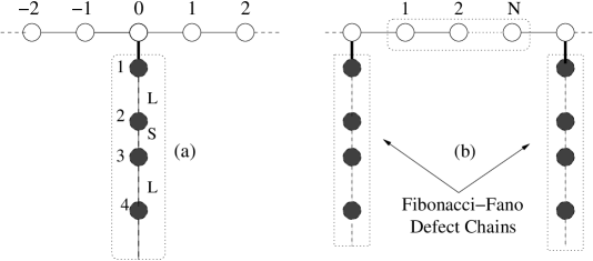
Figure 1: (a) The Fibonacci chain side coupled to a single site (b) The case of multiple grafted chains.

To calculate electronic transmission across the quantum wire, we use the real space renormalization group (RSRG) method south83 . We renormalize the hanging Fibonacci chain by decimating the internal sites selectively. For this we have to ‘fold’ the chain backwards by using the growth rule in opposite direction. To get unique recursion relation for the site at the chain’s lower boundary, we consider Fibonacci chains with odd index of generation only. Thus, instead of the growth rule, as pointed out before, we fold the chain by using the rule $LSL\rightarrow L^{\prime}$ and $LS\rightarrow S^{\prime}$, which is one step ahead of the usual deflation rule $L\rightarrow LS$ and $S\rightarrow L$. This is to be appreciated that, it is not a limitation of the scheme. As our interest is the large size behaviour of the impurity, by considering successive odd generations only of the Fibonacci chain we do not lose any physics whatsoever. Staring with a $2n+1$-th generation Fibonacci chain, decimation of $n$-steps folds it to a diatomic molecule with two end atoms having on-site potentials $\epsilon_{T,n}$ and $\epsilon_{B,n}$, and connected to each other by an effective hopping integral $t_{L,n}$. The process is outlined in the Appendix. Using this method, we can create a single, effective impurity with site potential $\epsilon^{*}$ sitting at the $0$-th site of the ordered backbone (quantum wire). The recursion relations are given by,

$$\epsilon_{\alpha,n} = \epsilon_{\alpha,n-1}+\frac{A_{n-1}}{D_{n-1}}+\frac{B_{n-1}}{D_{n-1}}$$

$$\epsilon_{\beta,n} = \epsilon_{\alpha,n-1}+\frac{t_{L,n-1}^{2}}{E_{\beta,n-1}}+\frac{B_{n-1}}{D_{n-1}}$$

$$\epsilon_{\gamma,n} = \epsilon_{\gamma,n-1}+\frac{t_{S,n-1}^{2}}{E_{\beta,n-1}}+\frac{A_{n-1}}{D_{n-1}}$$

$$\epsilon_{T,n} = \epsilon_{T,n-1}+\frac{A_{n-1}}{D_{n-1}}$$

$$\epsilon_{B,n} = \epsilon_{B,n-1}+\frac{B_{n-1}}{D_{n-1}}$$

$$t_{L,n} = \frac{t_{L,n-1}^{2}t_{S,n-1}}{D_{n-1}}$$

$$t_{S,n} = \frac{t_{L,n-1}t_{S,n-1}}{E_{\beta,n-1}}$$ (5)

where,

$$A_{n} = t_{L,n}^{2}E_{\gamma,n}$$

$$B_{n} = t_{L,n}^{2}E_{\beta,n}$$

$$D_{n} = E_{\beta,n}E_{\gamma,n}-t_{S,n}^{2}$$ (6)

Here, $E_{j}\equiv(E-\epsilon_{j})$ for $j=\alpha$, $\beta$ or $\gamma$. Finally, for the single impurity site we get,

$$\epsilon^{*}=\epsilon_{0}+\frac{t_{c}^{2}}{E-\tilde{\epsilon}}$$ (7)

where,

$$\tilde{\epsilon}=\epsilon_{T,n}+\frac{t_{L,n}^{2}}{E-\epsilon_{B,n}}$$ (8)

The problem is now reduced to calculating transmission across a single $\delta$-like impurity with an effective potential $\epsilon^{*}$. This is easily done kiv05 . The transmission coefficient is given by,

$$T=\frac{\alpha_{q}^{2}}{\alpha_{q}^{2}+1}$$ (9)

where, $\alpha_{q}=[2t_{0}(E-\tilde{\epsilon})\sin(qa)]/t_{c}$.

Figure 2: The transmission coefficient for (a) a periodic Fano defect with $21$ sites. The hopping integral in the defect chain has been taken to be equal to $0.5$ in unit of $t_{0}$. (b) Transmission coefficient for a Fibonacci-Fano defect in the $23$rd generation. We have selected $\epsilon_{j}=0$ with $j=\alpha$, $\beta$, $\gamma$. $t_{L}=t_{S}/2=0.5$ and $t_{c}=0.5$ in unit of $t_{0}$. The onsite potential $\epsilon_{0}$ and the hopping integral $t_{0}$ for the ordered quantum wire have been set equal to zero and one respectively. (c) The self similarity in the spectrum is highlighted.

Eq.(8) resembles the Fano formula (1), if we make the asymmetry parameter $\delta$ disppear. The resonance line width is,

$$\Gamma=\frac{t_{c}^{2}}{t_{0}\sin(q_{R}a)}$$ (10)

with $q_{R}$ corresponding to the wave vector at resonance. In this case, comparing with the Fano expression (1), we see that, $\omega=E-\tilde{\epsilon}$. $\tilde{\epsilon}$ is an energy dependent quantity. This, as we shall see, may give rise to asymmetric Fano profiles for a single hanging Fibonacci chain, as compared to a perfectly ordered chain.

III Results and discussion

We begin by considering a single Fibonacci-Fano defect. In Figs.2b and 2c we present results of the calculation of transmission coefficient across an effectively single defect that has been obtained after $n$-times renormalizing the Fibonacci chain of $2n+1$th generation. In particular, we discuss the ‘transfer model’ of the Fibonacci chain with $\epsilon_{\alpha}=\epsilon_{\beta}=\epsilon_{\gamma}=0$, and $t_{L}\neq t_{S}$. The energy spectrum of an infinite (or, semi-infinite) Fibonacci lattice with such specifications exhibits a three sub-band structure, each sub-band splitting up into three other sub-bands as one makes a closer scan in energy kkt83 . The result for an ordered chain is presented in Fig.2a for comparison. Transmission zeroes are obtained from the roots of the equation

$$E-\tilde{\epsilon}=0$$ (11)

At each real root of this equation $\epsilon^{*}\rightarrow\infty$, and a total reflection occurs. For all real roots the incoming electron faces an infinitely high potential barrier. Naturally, among these roots we are concerned about those, which fall in the allowed band of the ordered backbone. The electron can not be transmitted at these energies, and we get transmission zeroes. It should be appreciated that these roots also yield the discrete eigenvalues of the isolated Fibonacci chain. In the thermodynamic limit the eigenvalues of the Fibonacci chain are distributed in a Cantor set of measure zero kkt83 . Therefore, when the length of the side coupled Fibonacci-Fano defect increases to infinity, we expect a Cantor set distribution of transmission zeroes in the $T$ vs $E$ diagram. The hierarchical structure of the spectrum is apparent in the transmission profiles, as shown in Fig.2c. By tuning the values of the parameters it is possible to include the entire spectrum of the isolated defect chain in the allowed band of the ordered chain playing the role of the quantum wire. The fragmented character of the spectrum of the defect Fibonacci chain then allows one to control the conductance of the wire with the defect, as every subcluster exhibits windows of finite transmission separated from each other by abrupt Fano drops to zero.

Transmission resonances may be obtained from the solutions of the equation

$$E-\epsilon_{B,n}=0$$ (12)

This makes $\tilde{\epsilon}=0$, and $\epsilon^{*}=\epsilon_{0}$. Therefore, the ‘impurity’ in this case becomes indistinguishable from a site in the perfectly ordered quantum wire. For all such energy values the transmission coefficient $T=1$, independent of the wire-defect coupling $t_{c}$. The solutions of the equation $E-\epsilon_{B,n}$ are also distributed in a Cantor set structure.

An essential difference in the transmission spectrum offered by a quantum wire with an attached ordered chain kiv05 and that with a single attached Fibonacci-Fano defect is the observation of asymmetric Fano profiles. To appreciate the difference we look at the expanded form of the effective impurity potential, viz,

$$\epsilon_{0}^{*}=\epsilon_{0}+\frac{t_{c}^{2}[E-\epsilon_{B,n}]}{[E-\epsilon_{T,n}][E-\epsilon_{B,n}]-t_{L,n}^{2}}$$ (13)

As already noted, perfect transmission occurs at the energy eigenvalues satisfying Eq.(12) and, the transmission zeroes are obtained from the solution of $E-\tilde{\epsilon}=0$, or equivalently,

$$[E-\epsilon_{T,n}][E-\epsilon_{B,n}]-t_{L,n}^{2}=0$$ (14)

Owing to the highly fragmented nature of the spectrum of the isolated Fibonacci chain, any energy we hit upon will be arbitrarily close to a gap in the spectrum. As a result, for a big enough Fibonacci-Fano defect, $t_{L,n}$ (and, $t_{S,n}$ as well), after $n$ steps of renormalization will become vanishingly small. Thus, if we deviate slightly from the resonance energy by setting $E=\epsilon_{B,n}+\Delta$, with $\Delta$ being an arbitrarily small number that we can choose at our will, the left hand side of Eq.(12) can be made arbitrarily close to zero. But, at the same time, $t_{L,n}$ becomes very very small as well (for an appreciable size of the defect chain) , as the chosen energy, in all probability, will lie in a gap. Also, both $\epsilon_{T,n}$ and $\epsilon_{B,n}$ are of the same order of magnitude. Thus, the left hand side of Eq.(15) can be made to have a magnitude at least $\sim\bigcirc(\Delta^{2})$. This may make $\epsilon^{*}\rightarrow\infty$ and consequently, $T\rightarrow 0$ in the immediate neighborhood of a transmission resonance. This leads to the possibility of observing asymmetric profiles in the transmission spectrum with a Fibonacci-Fano defect chain. For an ordered chain as a defect, all the energy values extracted from the equation $E-\epsilon_{B,n}=0$ correspond to extended eigenstates of the chain (when isolated). As a consequence, the hopping integral under successive renormalization never flows to zero for any such energy. In the thermodynamic limit, the spectrum of the isolated chain will be a continuum. That is, any deviation from the roots of the equation $E-\epsilon_{B,n}=0$ will also be in the spectrum, and would correspond to an extended state. The hopping integral remains non zero for all such energies as well. This disapproves the juxtaposition of transmission zero and unit transmission, and hence an asymmetry in resonance profile. In Fig. 3 (bottom panel) we highlight the concommitant zeroes which give rise to the asymmetry in lineshape in case of a Fibonacci-Fano defect in its $15$th generation ($987$ bonds). The uniformity in spacing of the eigenvalues of an ordered Fano defect does not allow for any asymmetry. This is shown in Fig.3 (top panel).

The profile of the transmission window is sensitive to the choice of the wire-defect coupling $t_{c}$. For low $t_{c}$, we can have reasonably flat windows suddenly dropping down to provide zero transmission at $E=\tilde{\epsilon}$, while, with large enough values of $t_{c}$, the entire spectrum practically consists of sharp delta like transmission peaks arranged in a self similar triplet of clusters, typical of a Fibonacci lattice. The behavior is not difficult to understand if one remembers that $t_{c}$ is proportional to the width of resonance.

Before we end this section, it is worth mentioning that a non-zero flow of the hopping integrals , which usually implies the presence of extended eigenstates, may take place in a Fibonacci chain as well. One such energy, leading to a sharp asymmetric Fano resonance is shown in Fig.4. The defect chain is a $19$th generation Fibonacci lattice in the transfer model. Resonance takes place at $E=-0.03108$ in unit of $t_{0}$. The hopping integrals $t_{L,n}$ and $t_{S,n}$ do not flow to zero at this energy indicating that the corresponding eigenstate is not localized within the size of the defect.

Figure 3: The transmittivity ($T$) against energy when a $15$th generation ordered chain (top panel) and a Fibonacci chain (bottom panel) are side coupled. The positions of the resonance and anti-resonance are shown in each case by ‘asterix’ and a circle with a dot. The juxtaposition of the two symbols can be compared in the two cases. All the parameters are as in Fig.2

IV Multiple side coupled Defects

IV.1 Band Structure

In the spirit of Vasseur et al vas98 and Pouthier and Girardet pou02 we have investigated the effect of attaching muliple Fibonacci-Fano (FF) defects of identical size at regular interval on the ordered backbone. Just as in the case of an array of ordered side coupled chains vas98 , the FF defects, when grafted periodically along the backbone open up a series of absolute band gaps in the spectrum. For a Fibonacci chain in the $n$th generation we have $F_{n}$ bonds, and the band structure of an infinite array of grafted FF defects shows $F_{n}+N+1$ bands, where $N$ in the number of sites in the ordered backbone which separate two neighboring FF defects.

Figure 4: The sharply asymmetric Fano profile in the transmission spectrum of a $19$th generation Fibonacci chain attached to the wire. The values of on-site potentials and the hopping integrals are as in Fig.2, and $t_{c}=0.5$ in unit of $t_{0}$.

IV.2 Transmission Coefficient

A simple algebra leads to the most general expression for the transmission coefficient of identical $n$ grafted chains separated from each other by $N$ atoms in the backbone. Each chain is renormalized into a single defect sitting on the backbone and separated from its nearest defect by $N$ ‘pure’ sites. The system is further reduced, for convenience, to an array of identical pseudo-atoms by decimating the intermediate ‘pure’ sites. The new lattice spacing is now $(N+1)a$ and, the effective potential $\mu$ at each site as well as the effective nearest neighbour hopping integral $h$ are given by,

$$\mu = \epsilon^{*}+2t_{0}\frac{U_{N-1}(x)}{U_{N}(x)}$$

$$h = \frac{t_{0}}{U_{N}(x)}$$ (15)

where, $x=(E-\epsilon_{0})/2t_{0}$ and, $U_{j}$ is the $j$th order Chebyshev polynomial of the second kind. It is now straightforward to compute the transmission coefficient of $n$ such defects embedded in a perfect lead. The result is,

$$T=\frac{4\sin^{2}qa}{\left[-2U_{n+1}(y)+(rU_{n+2}(y)+\frac{U_{n}(y)}{r})\cos qa\right]^{2}+\left[rU_{n+2}(y)-\frac{U_{n}(y)}{r}\right]^{2}\sin^{2}qa}$$ (16)

where, $r=h/t_{0}$, and, $y=(E-\mu)/2h$. In Fig.5 we show transmission spectrum for more that two Fibonacci-Fano defect chains. Two such cases are presented with $t_{c}=0.1$ and $1.0$ in unit of $t_{0}$. In each case there are ten grafted chains separated by three sites of the backbone. Each grafted chain is a $15$th generation Fibonacci lattice containing $987$ bonds. With $t_{c}=0.1$, the absolute gaps are not formed with only $10$ chains. However, an increase in the value of $t_{c}$ to unity opens up gaps in the spectrum. With a small number of chains one may still look for asymmetric Fano profiles. However, quantum interference between the waves reflected back and forth between the grafted defect chains mask such resonances, and it is difficult to locate them numerically. The self similarity in the distribution of the eigenvalues of each defect, when they are decoupled from the backbone are lost as well.

Figure 5: Transmittivity (T) against energy (E) for ten $7$th generation Fibonacci-Fano defect chains grafted in the ordered backbone. The chains are spaced $3$ ‘pure’ sites apart. $t_{c}=0.1$ in (a), and $t_{c}=1.0$ in (b). Other parameters of the system are as in Fig.2.

Inversion of peak-dip positions: Two Fibonacci-Fano defects

We now address separately the problem of transmission through two defect chains spaced $N$ sites apart. It is found that, irrespective of whether the defect chain is quasiperiodic or not, at special values of energy the positions of resonance and the anti-resonance can be swapped by varying the number of ‘pure’ atoms in the backbone separating the hanging defects. Incidentally, a similar phenomenon was also reported in Ref.kiv05 when an additional impurity atom was placed in the main array. Thus, it is sensible to attribute this feature (in systems such as we address here) to the presnece of two defects in an ordered backbone, at least one of which is a Fano defect. The significance of such swapping has already been pointed out elsewhere voochu . For example, with a magnetic impurity, the transmission peak of the spin ‘up’ (down) electrons may coincide with the transmission zero of the spin ‘down’ (up) electrons. This opens up the possibility of desiging a spin filter with such systems. It may be mentioned that, tight binding model of a quntum wire with an attached tight binding ring has already been proposed as a model of a spin filtering device lee06 .

As an example of the above phenomenon, in Fig.6, we demonstrate the swapping of the peak-dip positions for two cases. Fig.6a corresponds to the simpler one, where each of the two defect chains consists of just two atoms coupled to the backbone at two different sites separated by $N$ intermediate atomic sites of the backbone. The zeroes of transmission are at, $E=\epsilon_{0}\pm t_{0}$. The swapping has been demonstrated around $E=\epsilon_{0}+t_{0}$ by changing $N$ from $N=3$ (solid line) to $N=4$ (dashed line). In Fig.6b, a similar transmission profile is exhibited for a Fibonacci-Fano defect with $21$ bonds. In each case, the swapping of the peak-dip profile takes place around a transmission-zero, which is obtained by solving the equation $E-\tilde{\epsilon}=0$. Using a Fibonacci chain as a Fano defect opens up the possibility of getting a fractal distribution of such inversion of the resonance-anti resonance positions. One can perhaps then think of a spin filter that can operate on arbitrarily narrow scales of energy. However, detecting such swapping of resonance profiles at various energies remains a non trivial task, as the spectra of the grafted chains, when quasiperiodic in character, offer a highly fragmented band structure. This aspect needs further attention.

Getting an anlytical insight into the phenomenon of swapping is difficult with big Fibonacci chains, as the expression for the transmission amplitude turns out to be a formidable one. However, we explicitly demonstrate that, for the case of the simpler diatomic chains, it is indeed possible to ‘see’ the effect as $N$ changes.

Let us look back at Fig.1b with just two atoms in each of the defect chains. We assign on-site potential $\epsilon_{0}$ to each atom in the two chains, while the inter-atomic hopping in each chain has a value $t_{0}$. The expression for $\tilde{\epsilon}$, defined in Eq.(8) now becomes,

$$\tilde{\epsilon}=\epsilon_{0}+\frac{t_{0}^{2}}{E-\epsilon_{0}}$$ (17)

With two such chains hanging $N$ atoms (of the backbone) apart, the problem is reduced to the calculation of electronic transmission through a system of $N+2$ atoms. The outer ones are the ‘impurity’ atoms, each with site energy $\epsilon^{*}$ defined in Eq.(7). The $N$ ‘inner’ atoms are ‘pure’, and have on-site potential equal to $\epsilon_{0}$. The nearest neighbour hopping integral is $t_{0}$ in this sample. The sample is then connected to two ideal semi-infinite leads at the two ends, and the transmission amplitude can be worked out in a straightforward way stone81 as,

$$\tau=\frac{e^{-ikNa}2i\sin ka}{\alpha+i\beta}$$ (18)

where, $\alpha=M_{11}+(M_{12}-M_{21})\cos ka-M_{22}\cos 2ka$, $\beta=(M_{12}-M_{21})\sin ka-M_{22}\sin 2ka$, and $M_{ij}$ are the elements of the transfer matrix stone81 ,

$$M=M_{imp}.M_{pure}^{N}.M_{imp}$$ (19)

Here, $M_{imp}$ and $M_{pure}$ stand for the transfer matrix across the ‘impurities’ and the ‘pure’ site respectively. The explicit form of $M$ is,

$$M=\left(\begin{array}[]{cc}(E-\epsilon^{*})/t_{0}&-1\\ 1&0\end{array}\right).\left(\begin{array}[]{cc}U_{N}(x)&-U_{N-1}(x)\\ U_{N-1}(x)&U_{N-2}(x)\end{array}\right).\left(\begin{array}[]{cc}(E-\epsilon^{*})/t_{0}&-1\\ 1&0\end{array}\right)$$ (20)

where, $U_{N}(x)$ stands for the $N$th order Chebyshev polynomial, already defined in Eq.(16). We now look at the behavior of the transmission amplitude in the neighborhood of a transmission zero, which we choose to be $E=\epsilon_{0}+t_{0}$. We set $E=\epsilon_{0}+t_{0}+\sigma$ and neglect terms $\sim\bigcirc(\sigma^{2})$ or more (compared to $\sigma$ or terms free from $\sigma$) in the expanded matrix elements $M_{ij}$. The approximate expression of the transmission amplitude, in the neighborhood of the transmission zero becomes,

$$\tau\sim\frac{4t_{0}ie^{-ikN}\sin k}{t_{c}^{2}(U_{N}(x)-U_{N-1}(x))}\frac{\sigma^{2}}{(\sigma-\frac{t_{c}^{2}}{2t_{0}}\frac{U_{N}(x)}{U_{N}(x)-U_{N-1}(x)})+i\sqrt{3}\frac{U_{N}(x)}{U_{N}(x)-2U_{N-1}(x)}\sigma}$$ (21)

The above expression immediately tells us that the ‘zero’ of the numerator occurs at $\sigma=0$ ($\sin k$ evaluated at the above energy is not going to be zero), while the zero of the real part of the denominator occurs at $\sigma=[t_{c}^{2}U_{N}(x)]/[2t_{0}(U_{N}(x)-U_{N-1}(x)]=\delta$(say). The locations of the two zeroes are different. This set of detuned zeroes results in a non-zero Fano parameter and an asymmetric resonance around $E=\epsilon_{0}+t_{0}$. The quantity $\delta$ plays the role of the non-zero Fano parameter in this case. A swapping of the peak-dip positions can take place if the Fano parameter $\delta$ flips sign with a change in the value of $N$. We have chekcked that this precisely is the case here, as $N$ changes from three to four. In fact, different pairs of values of $N$ can be obtained for which the asymmetry parameter flips sign. As a result, when $\delta>0$, the peak appears after the dip, and when $\delta<0$, the peak precedes the dip.

It is worth mentioning that, the transition from the pole-zero (or, equivalently, peak-dip) to zero-pole positions was also investigated for model quantum systems by several authors kim99 -vargia05 . The change in the asymmetry parameter was shown to be caused by a variation in some continuous parameter of the system, for example, the strength of the impurity in Ref.kim99 , or the magnetic flux in Ref.lad06 . On the other hand, in our case, the asymmetry parameter is a function of the discrete variable $N$, the number of sites between the two dangling chains. It is the change in the discrete variable $N$ that causes the interesting swapping in the peak-dip positions. We have tested for other cases also, namely, when each of the hanging chains contain three or four atoms. In each case, in a $\sigma$- neighborhood of a transmission zero, we find $\tilde{\epsilon}\sim 1/\sigma$, leading to a $N$-dependent Fano parameter that flips sign when $N$ is made to change suitably. The case of two Fibonacci-Fano defects has also been examined numerically, and the result indicates that it is true for this system as well. Thus, we get confidence to predict that, the swapping is a generic feature of two Fano defects. Whether this remains true when more defect chains are incorporated, needs to be examined carefully. It may be mentioned that similar Fano-like profiles are also found in cases where the distribution of stubs follows a quasiperiodic sequence samar04 -sheelan05 . However, the aspect of Fano effects in transmission was not addressed in any of these papers.

Before we end this section, a comment on the nature of the eigenstates will be in order. The most important thing to remember is that, to adjudge the character of an electronic state at a particular energy, one has to make sure that the energy concerned corresponds to an ‘allowed’ state of the full system, i.e. the sample plus the semi-infinite leads. This implies that, a consistent solution of the Schrödinger equation will exist at that energy all over the sample. It can be checked, at least for small Fano defects such as the case discussed above, by explicitly working out the amplitudes of the wave function at all sites of the system. It will be found that consistent solution can be obtained for various values of $N$, by assigning zero amplitude to the sites where the defect chains join the ordered backbone. The profile of amplitude will resemble a standing wave pattern between the potential barriers (existing at the defect-backbone junction points) whose height in given by $\tilde{\epsilon}$. At $E=\tilde{\epsilon}$, the effective potential $\epsilon^{*}$ becomes infinitely high. As a result, though a non-trivial distribution of amplitudes with finite values can be written throughout the system, the electronic transport reduces to zero. An electron , released in any one of the intermediate $N$ sites and in between the potential barriers, will be reflected back and forth. Beyond the well, however, one can have a perfectly periodic distribution of amplitudes. Thus, it is not right to call such states exponentially localized in the language of conventional localization studies. As the nearest neighbouring sites are still coupled by non-zero hopping integral, it may be tempting to call them extended states. But, this will also be wrong, as the transmission across the sample for such an energy is zero. In a previous work, in the context of transport through a Vicsek fractal, such states were encountered, and have been termed ‘atypically extended’ bb96 .

Figure 6: Transmittivity of a two-defect sytem. (a) Two identical sites form a defect chain. Two such chains are separated from each other by $N=3$ (solid line) and $N=4$ (dashed line) atoms. (b) Two seventh generation Fibonacci-Fano defect chains ($21$ bonds) are attached to two sites of the quantum wire. The number of sites separating the two chains is $N=3$ (solid line) and $N=6$ (dashed line). The parameters are, $\epsilon_{0}=0$, $t_{0}=1$, and, $\epsilon_{\alpha}=\epsilon_{\beta}=\epsilon_{\gamma}=0$, $t_{L}=1$, $t_{S}=2$ and $t_{c}=0.4$ in unit of $t_{0}$. The swapping of the resonance points are clearly seen.

V Conclusion

We have examined the effect of coupling a quasiperiodic chain of increasing length to an ordered backbone on the electronic transmission. The self similar spectrum of the side coupled chain leads to an interesting transmission spectrum across the ordered lattice comprising of continuous zones of finite transmission inter-connected by sharp asymmetric Fano drops to zero. This does not disregard the presence of Breit Wigner type of resonance profiles. But we have not discussed this. Within a framework of real space renormalization group method, we also discuss the band structure for an infinite array of FF defects. Finally the transmission properties when more than one FF defect chains are attached, are discussed. With two chains there is a swapping of Fano resonance profiles is observed at a specific energy. This has been explained using a simpler system. This aspect, as also observed earlier, may be utilised in designing novel spin filters.

Acknowledgement

I thank Santanu Maity for useful suggestions in preparing the manuscript and Samar Chattopadhyay for participating in some stimulating discussion.

APPENDIX

We briefly discuss the way to obtain Eq.(5) to Eq.(8). Real space decimation method (see sam02 , sheelan05 , and references therein) is used. The basic set of difference equations to be used has the general shape,

$$(E-\epsilon_{j})\psi_{j}=t_{j,j-1}\psi_{j-1}+t_{j,j+1}\psi_{j+1}$$ (22)

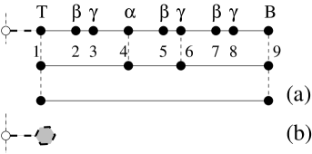
Figure 7: (a) Illustration of the basic decimation process. (b) Obtaining $\tilde{\epsilon}$ from the renormalized diatomic molecule.

where, $\psi_{j}$ stands for the amplitude of the wave function at the $j$th site and $t_{j,j\pm 1}$ represents the nearest neighbour hopping integral between the $j$th and the $j\pm 1$th site. As an illustration, we refer to Fig.8. $T$ stands for ‘top’ and $B$ stands for ‘bottom’ atoms in Fig.1. A Fibonacci chain with eight bonds ($5$th generation) is attached to a site of the backbone (marked by the open circle in Fig.8a). The set of difference equations for the Fibonacci chain are,

$$(E-\epsilon_{T})\psi_{1} = t_{c}\psi_{0}+t_{L}\psi_{2}$$

$$(E-\epsilon_{\beta})\psi_{2} = t_{L}\psi_{1}+t_{S}\psi_{3}$$

$$(E-\epsilon_{\gamma})\psi_{3} = t_{S}\psi_{2}+t_{L}\psi_{4}$$

$$(E-\epsilon_{\alpha})\psi_{4} = t_{L}\psi_{3}+t_{L}\psi_{2}$$

$$(E-\epsilon_{\beta})\psi_{5} = t_{S}\psi_{6}+t_{L}\psi_{4}$$

$$(E-\epsilon_{\gamma})\psi_{6} = t_{S}\psi_{5}+t_{L}\psi_{7}$$

$$(E-\epsilon_{\beta})\psi_{7} = t_{S}\psi_{8}+t_{L}\psi_{6}$$

$$(E-\epsilon_{\beta})\psi_{8} = t_{L}\psi_{9}+t_{S}\psi_{7}$$

$$(E-\epsilon_{B})\psi_{9} = t_{L}\psi_{8}$$ (23)

Here, $\psi_{0}$ implies the amplitude of wave function at the zeroth site of Fig.1 (which is the open circle here) where, the defect chain joins the back bone. The renormalization scheme $LSL\rightarrow L^{\prime}$ and $LS\rightarrow S^{\prime}$ implies that we eliminate the amplitudes at sites numbered $2(\beta)$, $3(\gamma)$, $5(\beta)$, $7(\beta)$ and $8(\gamma)$ in terms of the remaining sites. This brings the $8$-bond FF defect to an effectively $3$-bond Fibonacci chain with renormalized values of the site energies and the hopping integrals. Such a decimation scheme, when applied to a $2n+1$th generation Fibonacci chain, leads to the set of equations (5). Consequently, the top and the bottom sites, which remain un-decimated, also have renormalized values of the on-site potential. One further decimation of the two intermediate sites (the second stage in Fig.8a) brings the entire chain down to a diatomic molecule with renormalized ‘top’ and ‘bottom’ atoms. Finally, the amplitude at the bottom site is eliminated in terms of the amplitude at the top site to get the expression for $\tilde{\epsilon}$. This is depicted in Fig.8b. With bigger FF defect chains the renormalization process is continued, till the final diatomic molecule (Fig.8a) is obtained. Thus we get $\tilde{\epsilon}$ in Eq.(8).

References

- (1) D. Goldhaber-Gordon, H. Shtrikman, D. Mahalu, D. Abusch-Magder, U. Meirav, and M. A. Kastner, Nature (London) 391, 156 (1998); D. Goldhaber-Gordon, J. Göres, M. A. Kastner, H. Shtrikman, and D. Mahalu, Phys. Rev. Lett. 81, 5225 (1998).
- (2) S. M. Cronenwett, T. H. Oosterkamp, and L. P. Kouwenhoven, Science 281, 5 (1998).
- (3) W. Z. Shangguan, T. C. Au Yeung, Y. B. Yu, and C. H. Kam, Phys. Rev. B 63, 235323 (2001); A. W. Holleitner, R. H. Blick, A. K. Huttel, K. Eber, and J. P. Kotthaus, Science 297, 70 (2002).
- (4) N. Sundaram, S. A. Chalmers, P. F. Hopkins, and A. C. Gossard, Science 254, 1326 (1991).
- (5) P. Gambardella, M. Blanc, H. Brune, K. Kuhnke, and K. Kern, Phys. Rev. B 61, 2254 (2000); A. Dallmeyer, C. Carbone, W. Eberhardt, C. Pampuch, O. Rader, W. Gudat, P. Gamberdella, and K. Kern, Phys. Rev. B 61, R5133 (2000).
- (6) J. O. Vasseur, P. A. Deymier, L. Dobrzynski and J. Choi, J. Phys.:Condens. Matter 10, 8973 (1998).
- (7) V. Pouthier and C. Girardet, Phys. Rev. B 66, 115322 (2002).
- (8) P. A. Orellana, F. Dominguez-Adame, I. Gómez, and M. L. Ladrón de Guevara, Phys. Rev. B 67, 085321 (2003).
- (9) F. Dominguez-Adame, I. Gómez, P. A. Orellana, and M. L. Ladrón de Guevara, Microelec. Jour. 35, 87 (2004).
- (10) F. Guinea and J. A. Vergés, Phys. Rev. B 35, 979 (1987).
- (11) U. Fano, Phys. Rev. 124, 1866 (1961).
- (12) U. Fano and A. R. P. Rau, Atomic Collisions and Spectra (Academic Press, Orlando, 1986).
- (13) J. Faist, F. Capasso, C. Sirtori, K. W. West, and L. N. Pfeiffer, Nature (London), 390, 589 (1997).
- (14) F. Cerdeira, T. A. Fjeldly, and M. Cardona, Phys. Rev. B 8, 4734 (1973).
- (15) V. Madhavan, W. Chen, T. Jamneala, M. M. Crommie, and N. S. Wingreen, Science 280, 567 (1998); J. Li, W. -D. Schneider, R. Berndt, and B. Delley, Phys. Rev. Lett. 80, 2893 (1998).
- (16) G. D. Mahan, Many Particle Physics (New York, Plenum Press, 1993).
- (17) Andrey E. Miroshnichenko, Sergei F. Mingaleev, Sergej Flach, and Yuri S. Kivshar, Phys. Rev. E 71, 036626 (2005).
- (18) Andrey E Miroshnichenko and Yuri S. Kivshar, Phys. Rev. E 72, 056611 (2005).
- (19) M. L. Ladrón de Guevara, F. Claro, and P. A. Orellana, Phys. Rev. B 67, 195335 (2003).
- (20) P. A. Orellana, M. L. Ladrón de Guevara, and F. Claro, Phys. Rev. B 70, 233315 (2004).
- (21) M. Kohmoto, L. P. Kadanoff, and C. Tang, Phys. Rev. Lett. 50, 1870 (1983); M. Kohmoto, B. Sutherland, and C. Tang, Phys. Rev. B 35, 1020 (1987); J. B. Sokoloff, Phys. Rep. 126, 85 (1985).
- (22) E. Macia and F. Dominguez-Adame, Electrons, Phonons and Excitons in Low Dimensional Aperiodic Systems (Editorial Complutense, Madrid, 2000).
- (23) B. W. Southern, A. A. Kumar, and J. A. Ashraff, Phys. Rev. B 28, 1785 (1983).
- (24) Khee-Kyun Voo and Chon Saar Chu, Phys. Rev. B 72, 165307 (2005).
- (25) M. Lee and C. Bruder, Phys. Rev. B 73, 085315 (2006).
- (26) S. Chattopadhyay and A. Chakrabarti, Phys. Rev. B 65, 184204 (2002).
- (27) A. Douglas Stone, J. D. Joannopoulos, and D. J. Chadi, Phys. Rev. B 24, 5583 (1981).
- (28) C. S. Kim, A. M. Satanin, Y. S. Joe, and R. M. Cosby, Phys. Rev. B 60, 10962 (1999).
- (29) O. Olendski and L. Mikhailovska, Phys. Rev. B 67, 035310 (2003).
- (30) M. L. Ladrón de Guevara and P. A. Orellana, Phys. Rev. B 73, 205303 (2006).
- (31) V. Vargiamidis and H. M. Polatoglou, Phys. Rev. B 72, 195333 (2005).
- (32) S. Chattopadhyay and A. Chakrabart, J. Phys. Condens. Matter 16, 313 (2004).
- (33) S. Sengupta, A. Chakrabarti and S. Chattopadhyay, Phys. Rev. B 71, 134204 (2005).
- (34) A. Chakrabarti and B. Bhattacharyya, Phys. Rev. B 54 R12625 (1996).