Out-of-plane spin polarization from in-plane electric and magnetic fields

Abstract

We show that the joint effect of spin-orbit and magnetic fields leads to a spin polarization perpendicular to the plane of a two-dimensional electron system with Rashba spin-orbit coupling and in-plane parallel dc magnetic and electric fields, for angle-dependent impurity scattering or nonparabolic energy spectrum, while only in-plane polarization persists for simplified models. We derive Bloch equations, describing the main features of recent experiments, including the magnetic field dependence of static and dynamic responses.

Generating spin populations at a nanometer scale is one of the central goals of spintronics Wolf et al. (2001). Using spin-orbit interaction promises electrical control, allowing to integrate spin generation and manipulation into the traditional architecture of electronic devices. Bulk spin polarization, driven by electron drift in an electric field, was predicted long ago for noncentrosymmetric three- (3D) and two-dimensional (2D) systems Ivchenko and Pikus (1978); Vas’ko and Prima (1979); Levitov et al. (1985); Edelstein (1990); Aronov et al. (1991); Bernevig and Zhang (2005). In 2D, the polarization is in-plane, typically along the effective spin-orbit field $\mathbf{b}_{\mathrm{dr}}=\langle\mathbf{b}_{\mathrm{SO}}(\mathbf{k})\rangle\neq 0$, obtained by averaging spin-orbit coupling over the distribution of electron momenta $\hbar\mathbf{k}$ foo . In-plane polarization components were observed recently in $p$-GaAs heterojunctions Silov et al. (2004), quantum wells Ganichev et al. (2006), and strained $n$-InGaAs films Kato et al. (2004a). Out-of-plane spin polarization can be generated by the spin-Hall effect, but only near sample edges D’yakonov and Perel’ (1971). Below, we propose a mechanism for out-of-plane spin polarization generated in the bulk by applying an in-plane magnetic field $\mathbf{B}$. This perpendicular polarization allows efficient optical access, e.g., via Kerr rotation. We find that the use of such an average field $\mathbf{b}_{\mathrm{dr}}$ is not always valid. Naively, one might consider the system as being subject to a total in-plane field $\langle\mathbf{b}\rangle$, given by the sum of $\mathbf{B}$ and $\mathbf{b}_{\mathrm{dr}}$, see Fig. 1(a). In steady state, one then expects electrons to be polarized along this total field: in particular, no polarization perpendicular to the $\mathbf{b}_{\mathrm{dr}},\>\mathbf{B}$ plane. Algebraic addition of these fields worked well in describing Hanle precession of optically oriented 2D electrons in GaAs Kalevich and Korenev (1990). However, Kato et al. Kato et al. (2004a) reported a spin polarization that is incompatible with such a naive picture and emphasized the need of identifying its microscopic mechanisms.

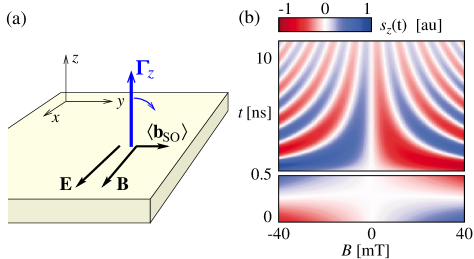
Figure 1: (color) (a) Field geometry, assuming $g\mu_{\mathrm{B}}>0,$ $\alpha<0$. Out-of-plane spin polarization is electrically generated with rate $\Gamma_{z}$ (blue arrow) due to the interplay between spin-orbit interaction, external electric field $\mathbf{E}$ and magnetic field $\mathbf{B}$, and anisotropic impurity scattering. The polarization precesses (blue arc) in $g^{*}\mu_{\mathrm{B}}\mathbf{B}+\langle\mathbf{b}_{\mathrm{SO}}\rangle$. (b) Dynamics of out-of-plane component of spin polarization generated by a short electrical pulse of length $t_{p}\lesssim 1\>\mathrm{ns}$, for $\tilde{\gamma}_{0}=0.03$, $g^{*}=0.65$ and $\tau_{z}=5\>\mathrm{ns}$. This pattern of spin polarization is in agreement with the experimental data of Fig. 4(c), Ref. Kato et al., 2004a.

In this article, we develop a theory describing the interplay between spin-orbit interaction and external electric and magnetic fields in the presence of impurity scattering, and demonstrate that the concept of average spin-orbit field is subject to severe restrictions. The naive expectation turns out to be correct only in the special case of parabolic bands and isotropic impurity scattering. However, as we show below, for anisotropic scattering (e.g., small angle scattering), such correlations result in a more complex structure of the distribution function and an out-of-plane spin polarization. Concretely, interplay of $\mathbf{b}_{\mathrm{dr}}$ and $\mathbf{B}$ leads to a generation term in the Bloch equation proportional to $\mathbf{b}_{\mathrm{dr}}\times\mathbf{B}$ whose magnitude is controlled by anisotropy of potential scattering and non-parabolicity of the energy spectrum. Remarkably, while this does not change the symmetry of the Hamiltonian, the symmetry of responses is lower than in the special case (and in the naive picture). Our results give a microscopic explanation of experiments Kato et al. (2004a) and provide a novel mechanism for generating spin polarization electrically via spin-orbit interaction.

We consider a model of 2D electrons with charge $e<0$ and (pseudo-) spin $\frac{1}{2}$, obeying a Hamiltonian

$$H=\epsilon_{k}-{\textstyle\frac{1}{2}}\mathbf{b}\left(\mathbf{k}\right)\cdot\boldsymbol{\sigma}+V\left(\mathbf{r}\right),$$ (1)

where $\epsilon_{k}$ is the dispersion law in the absence of spin-orbit coupling, $V\left(\mathbf{r}\right)$ is the potential due to impurites, $V_{\mathrm{i}}(\mathbf{r})$, plus a small electric field $\mathbf{E}$, $\boldsymbol{\sigma}$ are the Pauli spin matrices, and $\mathbf{b}\left(\mathbf{k}\right)$ includes both intrinsic spin-orbit field $\mathbf{b}_{\mathrm{SO}}(\mathbf{k})$ and external field $\mathbf{B}$. We consider in-plane magnetic field, i.e., there is no orbital quantization, and disregard electron-electron interaction. In the following, we study spin polarization density $\mathbf{s}\left(\mathbf{r}\right)=\left\langle\boldsymbol{\sigma}\right\rangle n_{2\mathrm{D}}$ and spin currents $\mathbf{j}^{\mu}\left(\mathbf{r}\right)=\langle{\textstyle\frac{1}{2}}\,\{\sigma_{\mu},\>\mathbf{v}\}\rangle n_{2\mathrm{D}}$. Here, $n_{2\mathrm{D}}$ is the electron density, $\left\{\,,\,\right\}$ is the anticommutator, and the velocity $\mathbf{v}=i\left[H,\,\mathbf{r}\right]$ is spin-dependent. (We set $\hbar=1$.)

For a bulk 2D system with only intrinsic spin-orbit interaction, the kinetic equation has been derived Aronov et al. (1991); Khaetskii (2006); Shytov et al. (2006). Following Ref. Shytov et al., 2006, we may write a spin-dependent Boltzmann equation for the distribution function, represented as a $2\times 2$ spin matrix $\hat{f}=\hat{f}_{0}(\mathbf{k})+\frac{1}{2}f_{\mathrm{c}}(\mathbf{k})\,1\!\!1+\mathbf{f}(\mathbf{k})\cdot\boldsymbol{\sigma}$, with equilibrium distribution function $\hat{f}_{0}$, excess particle density $f_{\mathrm{c}}$, $\mathbf{k}=(k_{x},\>k_{y})=(k\cos\varphi,\>k\sin\varphi)$, and spin polarization density described by $\mathbf{f}$. Magnetic field and spin-orbit coupling split the energy spectrum into two branches: for a given energy $\epsilon$, there are two Fermi surfaces. Thus, for elastic scattering, energy $\epsilon$ is conserved but $\left|\mathbf{k}\right|$ is not, due to inter-branch scattering. In the following, we assume $b\ll E_{\mathrm{F}}$. This motivates defining $k_{\epsilon}$ such that $\epsilon_{k_{\epsilon}}=\epsilon$, and defining $v_{\epsilon}=\epsilon_{k_{\epsilon}}^{\prime}$. For a fixed energy $\epsilon$, the velocity operator is epa

$$\mathbf{v}=\hat{\mathbf{k}}\>\left[v_{\epsilon}+\left(1+\zeta\right)\mathbf{b}\cdot\boldsymbol{\sigma}/2k_{\epsilon}\right]-(1/2)\,\partial(\mathbf{b}\cdot\boldsymbol{\sigma})/\partial\mathbf{k},$$ (2)

with unit vector $\hat{\mathbf{k}}=\mathbf{k}/k$ and band nonparabolicity $\zeta=(k_{\epsilon}/v_{\epsilon})(\partial v_{\epsilon}/\partial k_{\epsilon})-1$. Instead of using the distribution function $\hat{f}\left(\mathbf{k}\right)$ as density in $\mathbf{k}$-space, we consider it as a function of energy $\epsilon$ and direction $\varphi$ in $\mathbf{k}$-space. In this representation, $f_{\mathrm{c}}\left(\mathbf{k},\,\epsilon\right)$ and $\mathbf{f}\left(\mathbf{k},\,\epsilon\right)$ are transformed into distribution functions $n\left(\varphi,\,\epsilon\right)$ and $\boldsymbol{\Phi}\left(\varphi,\,\epsilon\right)$, resp., which can be written as a matrix $\hat{\Phi}\left(\varphi,\,\epsilon\right)$; for a detailed derivation see Ref. Shytov et al., 2006. The kinetic equation for $\mathbf{E}=E\mathbf{\hat{x}}$ is Shytov et al. (2006)

$$\frac{\partial\hat{\Phi}}{\partial t}+\boldsymbol{\sigma}\cdot\left[\mathbf{b}\times\boldsymbol{\Phi}-\frac{n}{4v_{\epsilon}}\,\mathbf{b}\times\frac{\partial\mathbf{b}}{\partial k}\right]+\frac{eE}{\left(2\pi\right)^{2}}\,\frac{\partial f_{0}}{\partial\epsilon}$$

$$\times\bigg{[}k_{x}+\frac{1}{2v_{\epsilon}}\frac{\partial}{\partial\varphi}\left(\mathbf{b}\cdot\boldsymbol{\sigma}\,\sin\varphi\right)\bigg{]}={\left(\frac{\partial\hat{\Phi}}{\partial t}\right)\negthickspace,\negmedspace\negthickspace}_{\mathrm{coll.}}$$ (3)

where $f_{0}$ is the Fermi distribution function, $\mathbf{b}=\mathbf{b}(\varphi)$ is evaluated for $\left|\mathbf{k}\right|=k_{\epsilon}$, and with charge distribution $n=8\beta\tau v_{\epsilon}k_{\epsilon}\cos\varphi$ and $\beta=(eE/16\pi^{2}v_{\epsilon})\,(-\partial f_{0}/\partial\epsilon)$. In Eq. (3), the first term is the partial time-derivative, the second term describes spin precession in the momentum dependent field $\mathbf{b}\left(\varphi\right)$, and the third term is the driving term, given in lowest order in $\mathbf{E}$.

The collision integral on the r.h.s. of Eq. (3) can be found in Born approximation by Golden Rule Shytov et al. (2006),

$$\left(\frac{\partial\hat{\Phi}(\varphi)}{\partial t}\right)_{\mathrm{coll}}=\int_{0}^{2\pi}d\varphi^{\prime}\>K(\vartheta)\left[\hat{\Phi}(\varphi^{\prime})-\hat{\Phi}(\varphi)\right]$$

$$+\int_{0}^{2\pi}d\varphi^{\prime}\>\boldsymbol{\sigma}\cdot\left[\mathbf{M}\left(\varphi,\varphi^{\prime}\right)n\left(\varphi^{\prime}\right)-\mathbf{M}\left(\varphi^{\prime},\varphi\right)n\left(\varphi\right)\right].$$ (4)

Here, the first term describes spin-independent scattering, with $K\left(\vartheta\right)=K\left(\varphi^{\prime}-\varphi\right)=W\left(q\right)k_{\epsilon}/2\pi\hbar^{2}v_{\epsilon}$ and $q=2k_{\epsilon}\sin\left(\left|\vartheta\right|/2\right)$. The factor $W(q)=\big{\langle}\left|V_{\mathrm{i}}(\mathbf{q})\right|^{2}\big{\rangle}$ does not depend on the direction of the momentum transfer $\mathbf{q}$ since we assume that the system is macroscopically isotropic. The second term in Eq. (4), described by Eq. (31) of Ref. Shytov et al., 2006, includes two contributions, arising from the spin-dependences of the density-of-states and of the momentum transfer for a fixed energy $\epsilon$. These contributions are proportional to $K\left(\vartheta\right)$ and $\tilde{K}\left(\vartheta\right)\equiv(dK/d\vartheta)\,\tan\left(\vartheta/2\right)$, resp., and explicitly depend on $\varphi,\>\varphi^{\prime}$ through $\mathbf{b}\left(\varphi\right)$ and $\mathbf{b}\left(\varphi^{\prime}\right)$.

We consider Rashba spin-orbit interaction, and choose the $x$ axis along the field $\mathbf{B}$, i.e.,

$$\mathbf{b}\left(\mathbf{k}\right) =2\alpha\,\hat{\mathbf{z}}\times\mathbf{k}+\Delta_{x}\,\hat{\mathbf{x}},\qquad\Delta_{x}=g^{*}\mu_{\mathrm{B}}B,$$ (5)

with Zeeman splitting $\Delta_{x}$, thus $\mathbf{b}\left(\mathbf{k}\right)$ is in-plane and $\mathbf{E}$ and $\mathbf{B}$ are parallel, see Fig. 1(a). (For $\mathbf{E}=E\mathbf{\hat{y}}$ there is $yz$ mirror symmetry and $s_{z}$ vanishes. Thus, the $s_{z}$ term linear in $\mathbf{E}$ is determined only by the component $E_{x}$ parallel to $\mathbf{B}$.)

Next, we write the kinetic equation (3) in Fourier space by expanding the azimuthal dependence as $f\left(\varphi\right)=\sum_{m=-\infty}^{\infty}e^{im\varphi}\,f_{m}.$ Combining the in-plane spin distribution as $\Phi^{x}(\varphi)+i\Phi^{y}(\varphi)=\sum_{m}e^{im\varphi}\,\Psi_{m}$, and using the form of $\mathbf{M}$ given in Ref. Shytov et al., 2006 we find epa

$$\dot{\Psi}_{m} =i\Delta_{x}\Phi_{m}^{z}+ib_{\alpha}\Phi_{m-1}^{z}+b_{\alpha}\beta\left(2+\tilde{\gamma}_{\left(+\right)}\right)\delta_{m,2}$$

$$+\Delta_{x}\beta\left(1+\tilde{\gamma}_{0}\right)\delta_{\left|m\right|,1}-\tau^{-1}k_{m}\Psi_{m},$$ (6)

$$\dot{\Phi}_{m}^{z} =\frac{i}{2}\,b_{\alpha}^{*}\Psi_{1+m}-\frac{i}{2}\,b_{\alpha}\Psi_{1-m}^{*}+i\,\frac{\Delta_{x}}{2}\left(\Psi_{m}-\Psi_{-m}^{*}\right)$$

$$+\Delta_{x}\left|b_{\alpha}\right|\tau\beta\,\Big{(}\delta_{m,0}+\frac{1}{2}\,\delta_{\left|m\right|,2}\Big{)}-\tau^{-1}k_{m}\Phi_{m}^{z},$$ (7)

with inverse transport time $\tau^{-1}=2\pi\left(K_{0}-K_{1}\right)$ and $k_{m}=(K_{0}-K_{m})/(K_{0}-K_{1})$. Also, $b_{\alpha}=2i\alpha k$, so the spin-orbit field can be written as $b_{x}+ib_{y}\big{|}_{B=0}=b_{\alpha}e^{i\varphi}$. Finally, the remaining parameters are

$$\tilde{\gamma}_{\left(+\right)}=2(k_{2}-1),\quad\;\tilde{\gamma}_{0}=\zeta+2\,\frac{\tilde{K}_{1}-\tilde{K}_{0}}{K_{0}-K_{1}}.$$ (8)

In the limit of small-angle scattering, $\tilde{\gamma}_{0}=\zeta+3.$ We have assumed that $\mathbf{B}$ is time-independent and any time-dependence of $\mathbf{E}$ is slow compared to $\tau^{-1}$.

Let us consider general properties of Eqs. (6)-(7). One can prove algebraically that

$$\Phi_{m}^{z}={\Phi_{-m}^{z}}^{*}=\left(-1\right)^{m}\Phi_{-m}^{z},\quad\Psi_{m}=-\left(-1\right)^{m}\Psi_{m}^{*}$$ (9)

for both the stationary regime and for transients generated by a time-dependent electric field. [Arbitrary initial conditions might deviate from Eq. (9), but such deviations would decay to zero at least as fast as the spin relaxation rate.] Also, these identities directly follow from the symmetry properties of the components of the pseudovector $\boldsymbol{\Phi}$ for the system with the axial symmetry $C_{\infty v}$ of the Rashba spin-orbit coupling in the fields $\mathbf{E},\>\mathbf{B}\parallel\hat{\mathbf{x}}$.

In particular, the symmetry of Eq. (9) allows $\Phi_{0}^{z}\neq 0$ in the stationary regime; therefore the spin polarization $s_{z}$ is generally finite, despite the fact that the effective field $\mathbf{b}(\mathbf{k})$ has only in-plane components. Now we can evaluate Eq. (6) for all $m$ and Eq. (7) for $m\geq 0$, and eliminate complex conjugated quantities using Eq. (9).

Isotropic scattering, parabolic bands, stationary regime. First, we assume isotropic scattering and parabolic bands, thus $\tilde{K}_{m}=0$ and

$$\tilde{\gamma}_{\left(+\right)},\tilde{\gamma}_{0}=0,\qquad k_{m}=1-\delta_{m,0}.$$ (10)

In this case, we solve the kinetic equations (6)-(7) exactly by setting $\partial\boldsymbol{\Phi}/\partial t=0$. The stationary solution is

$$\Psi_{m}^{\mathrm{is}} =\Delta_{x}\tau\beta\delta_{\left|m\right|,1}+2b_{\alpha}\tau\beta\left(\delta_{m,0}+\delta_{m,2}\right),$$ (11)

$$\Phi_{m}^{z,\,\mathrm{is}} =0,$$ (12)

which can be checked by inspection. The total spin polarization density is $\mathbf{s}=\mathbf{s}^{\mathrm{eq}}+\mathbf{s}^{E}$, with equilibrium contribution $\mathbf{s}^{\mathrm{eq}}\parallel\mathbf{B}$ and non-equilibrium contribution $s^{E}_{\mu}=4\pi\int d\epsilon\>\Phi_{0}^{\mu}$. Thus, the out-of-plane polarization vanishes, $s_{z}=0$, as one would expect from the above naive argument—even though the symmetry allows $s_{z}\neq 0$. Hence, vanishing $s_{z}$ is a property of the specific model of Eq. (10). On the other hand, even for this model, our solution is $\boldsymbol{\Phi}(\varphi)=4\tau\beta\left[\mathbf{b}(\varphi)-\frac{1}{2}\Delta_{x}\hat{\mathbf{x}}\right]\cos\varphi$, i.e., in addition to the total field $\mathbf{b}$, there is a correction $-\frac{1}{2}\Delta_{x}\hat{\mathbf{x}}$, indicating that spin-orbit and external magnetic fields cannot be added. However, it does not contribute to the in-plane spin polarization, as it is averaged out when integrating over $\varphi$.

The polarization $s^{\mathrm{eq}}_{x}$, in the absence of spin-orbit coupling, arises from Pauli paramagnetism, $s^{\mathrm{eq}}_{x}=n_{\uparrow}-n_{\downarrow}=\frac{1}{2}\nu(\epsilon_{\downarrow}-\epsilon_{\uparrow})=\frac{1}{2}\nu\Delta_{x}$, with the density of states $\nu=k_{\mathrm{F}}/\pi v_{\mathrm{F}}=m^{*}/\pi$, Fermi momentum $k_{\mathrm{F}}$, Fermi velocity $v_{\mathrm{F}}$, and effective mass $m^{*}$. This spin polarization does not depend on the electric field, thus $\Phi_{0}^{x}=0$. On the other hand, the electric field causes drift, producing an average spin-orbit splitting, $b_{\mathrm{dr}}^{y}=\langle b_{y}\rangle=(1/n_{2\mathrm{D}})\iint d\epsilon d\varphi\,n(\epsilon,\varphi)\,b_{y}=2\alpha eE_{x}\tau.$ By analogy to Pauli paramagnetism, one might guess that $s^{E}_{y}=\frac{1}{2}\nu\langle b_{y}\rangle$. This expectation is indeed met, because $s^{E}_{y}=\alpha eE_{x}\tau\nu$ coincides with the value following from Eq. (11), and it also agrees with known $B=0$ results Vas’ko and Prima (1979); Edelstein (1990); Aronov et al. (1991); Bernevig and Zhang (2005); Inoue et al. (2004). Hence, for the model of Eq. (10), the in-plane polarization can be described in terms of the average spin-orbit field.

In the field $\Delta_{x}$, the equilibrium spin polarization per electron is $\frac{1}{2}\nu\Delta_{x}/n_{2\mathrm{D}}=\Delta_{x}/2E_{\mathrm{F}}$, so one expects that the drift caused by the charge current leads to a spin current $j_{x}^{x}=(j_{x}^{\mathrm{c}}/e)\,\Delta_{x}/2E_{\mathrm{F}}$. Our results agree with this expectation; evaluating the definition of $j_{x}^{x}$ by inserting $\mathbf{v}$ leads to $j_{x}^{x}=2\pi\int d\epsilon\>v_{\epsilon}\,\mathrm{Re}\left[\Psi_{1}+\Psi_{-1}+2\beta\Delta_{x}\tau\right]$ epa , then Eqs. (9) and (11) are used. Note that the spin current $j_{x}^{x}$ is well defined for $b_{\alpha}=0$ because spin is conserved; also our calculations with finite $b_{\alpha}$ result in the same $j_{x}^{x}$. Other spin current components $j_{\nu}^{\mu}$ vanish, even for finite $b_{\alpha}$; for $\Delta_{x}=0$ it is well-known that $j_{y}^{z}=0$ Inoue et al. (2004); Mishchenko et al. (2004); Burkov et al. (2004); Raimondi and Schwab (2005); Chalaev and Loss (2005); Dimitrova (2005); Krotkov and Das Sarma (2006).

Anisotropic Scattering and Bloch equations. Now we consider anisotropic scattering and/or non-parabolic bands, and also include transients. We consider the “dirty limit,” $\left|b_{\alpha}\right|\ll\tau^{-1}\ll E_{\mathrm{F}}$ with constant $\mathbf{B}$ such that $\tau_{z}=\frac{1}{2}\tau_{xy}=1/\left|b_{\alpha}\right|^{2}\tau$

$$\left|\omega\right|,\>\tau_{z}^{-1},\>\left|\Delta_{x}\right|\ll\left|b_{\alpha}\right|\ll\tau^{-1},$$ (13)

where $\omega$ is the characteristic frequency of the field $\mathbf{E}$, and $\tau_{z}=\frac{1}{2}\tau_{xy}=\big{(}|b_{\alpha}|^{2}\tau\big{)}^{-1}$ are the Dyakonov-Perel spin relaxation times. In this regime, $\Phi_{m}^{z}$ and $\Psi_{m}$ decay exponentially fast with increasing $|m|$, since $\delta\Phi_{m}^{z}/\delta\Phi_{m-1}^{z}\sim\tau^{2}b_{\alpha}\Delta_{x}\ll 1$ for $m\geq 2$, and similarly for $\Psi_{m}$. This allows us to solve kinetic equations (6)-(7) order-by-order in the small parameter $(\tau/\tau_{z})^{1/2}$. Considering the lowest non-vanishing order, it is sufficient to retain only equations for $|m|\leq 2$. Eliminating the $m=\pm 1,\,\pm 2$ components yields the equations of motion for $\boldsymbol{\Phi}$ up to order $(\tau/\tau_{z})^{1/2}$ epa .

Finally, we evaluate the equations of motion for the total polarization $\mathbf{s}$ at low temperature $T$, taking all parameters at the Fermi level. We obtain the Bloch equation

$$\mathbf{\dot{s}} =\left\langle\mathbf{b}\right\rangle\times\mathbf{s}-{\overleftrightarrow{\tau}{}_{\mathrm{s}}^{-1}}\,\mathbf{s}+\boldsymbol{\Gamma},$$ (14)

where the spin relaxation tensor ${\overleftrightarrow{\tau}{}_{\mathrm{s}}^{-1}}$ is diagonal with components $\{\tau_{xy}^{-1},\,\tau_{xy}^{-1},\,\tau_{z}^{-1}\}$ and $\boldsymbol{\Gamma}=\big{(}\frac{1}{2}\nu\Delta_{x}\,\tau_{xy}^{-1},\>\frac{1}{2}\nu\left\langle b_{y}\right\rangle\tau_{xy}^{-1},\>\frac{1}{4}\nu\Delta_{x}\left\langle b_{y}\right\rangle\tilde{\gamma}_{0}\big{)}$. Note that our proof of Eq. (14) is valid only in linear order in $\mathbf{E}$ [cf. Eq. (3)], i.e., products $\left\langle b_{y}\right\rangle s^{E}_{\mu}$ were disregarded.

To develop a physical picture for this central result, we note that Eq. (14) is a Bloch equation, where polarization $\mathbf{s}$ is generated with a rate $\Gamma$ and then precesses in the total field $\left\langle\mathbf{b}\right\rangle=g^{*}\mu_{\mathrm{B}}\mathbf{B}+\mathbf{b}_{\mathrm{dr}}$ (Hanle effect). Most remarkably, for anisotropic scattering and/or band nonparabolicity, the combined effect of spin-orbit and external fields generates a spin polarization along the $z$ axis with rate $\Gamma_{z}=\>\frac{1}{4}\nu\,g^{*}\mu_{\mathrm{B}}(\mathbf{B}\times\langle\mathbf{b}_{\mathrm{SO}}\rangle)_{z}\,\tilde{\gamma}_{0}=\frac{1}{2}\nu\alpha eE_{x}\tau\,\Delta_{x}\,\tilde{\gamma}_{0}$, i.e., perpendicular to both magnetic and spin-orbit fields. This rate $\Gamma_{z}$ arises as follows. Scattering of nonequilibrium carriers leads to an extra $k_{x}$-dependent $x$ polarization due to the term proportional to $\tilde{\gamma}_{0}$ in Eq. (6). On a timescale of $\tau$, this polarization then precesses around the $y$ component of $\mathbf{b}_{\mathrm{SO}}$, as described by the first two terms of Eq. (7).

Next we consider the dc case, $\mathbf{\dot{\mathbf{s}}}=0$. In the lowest order in $\mathbf{E}$, the total spin polarization is $s_{x}=\frac{1}{2}\nu\Delta_{x}$,

$$s_{y} =\frac{1}{2}\nu\alpha\,eE_{x}\tau\left[2+\frac{\Delta_{x}^{2}\tau_{xy}\tau_{z}}{1+\Delta_{x}^{2}\tau_{xy}\tau_{z}}\,\tilde{\gamma}_{0}\right],$$ (15)

$$s_{z} =\frac{1}{2}\nu\alpha\,eE_{x}\tau\>\frac{\Delta_{x}\tau_{z}}{1+\Delta_{x}^{2}\tau_{xy}\tau_{z}}\,\tilde{\gamma}_{0}.$$ (16)

The first term of Eq. (15) arises from Eq. (11), while the second term and $s_{z}$ are due to anisotropic scattering or nonparabolic bands. The dependence of $s_{z}$ on $\Delta_{x}$ is in agreement with the data in Fig. 1c of Ref. Kato et al., 2004a, where $\tau_{\mathrm{s}}=(\tau_{xy}\tau_{z})^{1/2}\approx$ 5 ns, suggesting that our microscopic model might explain the experimental observations.

Spin currents. Evaluating Eq. (6) for $m=0$, we find that $\Phi_{-1}^{z}=-(\Delta_{x}/b_{\alpha})\Phi_{0}^{z}$. We then evaluate the spin current at $T=0$, $j_{y}^{z}=4\pi\int d\epsilon\>v_{\epsilon}\,\mathrm{Im}\Phi_{-1}^{z}=4\pi\int d\epsilon\>v_{\epsilon}(\Delta_{x}/|b_{\alpha}|)\,\Phi_{0}^{z}=v_{\mathrm{F}}(\Delta_{x}/|b_{\alpha}|)\,s_{z}$, finding that $j_{y}^{z}$ is proportional to $s_{z}$. (This relationship also follows from the Heisenberg equation of $\dot{\sigma}_{y}$.) Hence, the polarization $s_{z}$ [Eq. (16)] leads to a transverse spin current $j_{y}^{z}$; a finite $j_{y}^{z}$ is in agreement with numerical results of Ref. Lin et al., 2006. For $\Delta_{x}=0$, this relation is equivalent to the argument Dimitrova (2005); Chalaev and Loss (2005) based on equations of motion Burkov et al. (2004), showing that $j_{y}^{z}=0$.

Spin Dynamics. Even for isotropic scattering, a time-dependent electric field leads to an out-of-plane polarization $s_{z}(\omega)=\frac{i}{2}\omega\nu\Delta_{x}b_{\mathrm{dr}}^{y}(\omega)/[\Delta_{x}^{2}-\omega^{2}+\tau_{\mathrm{s}}^{-2}-i(\tau_{xy}^{-1}+\tau_{z}^{-1})\omega]$; however, it has no static component $s_{z}(\omega=0)$. Similar results were found in Ref. Duckheim and Loss, 2006 for $\left|b_{\alpha}\right|\ll\Delta_{x},\,\tau^{-1}$.

Spin dynamics is accessible in a pump-probe scheme Kato et al. (2004a). Namely, spins can be pumped by applying a short electric pulse of duration $t_{\mathrm{p}}\ll\tau_{z},\,\Delta_{x}^{-1}$. Then, according to Eq. (14), the spin polarization immediately after the pulse is $s_{z}(0)=t_{\mathrm{p}}\,\Gamma_{z}\propto\Delta_{x}\tilde{\gamma}_{0}$, i.e., $s_{z}(0)$ is an odd function of $\Delta_{x}$. Solving the Bloch equation (14), we get

$$s_{z}(t)=s_{z}(0)\,e^{-3t/4\tau_{z}}\left[\cos\Omega t-\frac{1+2/\tilde{\gamma}_{0}}{4\Omega\tau_{z}}\,\sin\Omega t\right]$$ (17)

with frequency $\Omega=\sqrt{(4\Delta_{x}\tau_{z})^{2}-1}/4\tau_{z}$ of Hanle oscillations (for consistency, we only consider terms linear in $\mathbf{E}$). We plot $s_{z}(t)$ in Fig. 1(b), taking the parameters of Ref. Kato et al., 2004a and with a choice of $\tilde{\gamma}_{0}=0.03$, and find qualitative agreement with the experiment. The weak-field region $4|\Delta_{x}|\tau_{z}<1$, where the oscillations are overdamped, is very narrow, $|B|\lesssim 0.25\>\mathrm{mT}$. Note that the experimental data shows that the sign of $s_{z}$ depends on the sign of $\Delta_{x}$, already on time scales much shorter than $|\Delta_{x}|^{-1}$. Therefore, the sign of $s_{z}$ cannot be due to spin precession in the external magnetic field—implying that a polarization generation mechanism like the one described above was experimentally observed in Ref. Kato et al., 2004a.

Strictly speaking, quantitative comparison with the data of Ref. Kato et al., 2004a cannot be performed because the films were of low mobility $E_{\mathrm{F}}\tau\sim 1$, violating the assumptions of our Boltzmann description, and were in 3D regime (a coupling $k_{y}\sigma_{x}-k_{x}\sigma_{y}$ occurs here due to strain). Furthermore, in models with a more complicated spin-orbit interaction than the Rashba coupling, other sources of $z-$polarization might become important. However, Eq. (13) was satisfied, because $\hbar/\tau_{z}\sim 3\times 10^{-8}\>\mathrm{eV}$; $\left|\Delta_{x}\right|\lesssim 10^{-6}\>\mathrm{eV}$; $|b_{\alpha}|\sim 10^{-5}\>\mathrm{eV}$; and $\hbar/\tau\sim 2\times 10^{-3}$ eV Kato et al. (2004a, b).

The effective field $\mathbf{b}(\mathbf{k})$ for a 2DEG with pure linear Dresselhaus coupling, on the $(001)$ surface of a III-V material, is obtained by replacing $\mathbf{k}$ on the right hand side of Eq. (5) by $\mathbf{q}\equiv\mathcal{R}\mathbf{k}$, where $\mathcal{R}$ denotes reflection through the $(110)$ crystal plane. Our result (16) for the polarization $s_{z}$ can be applied to this case if we replace $E_{x}$ by the component of the electric field along the direction $\mathbf{B}^{\prime}\equiv\mathcal{R}\mathbf{B}$. For general forms of the spin orbit coupling, we note that the $\mathrm{C}_{2v}$ symmetry of the system ensures that if $B=0$, there can be no term in $s_{z}$ linear in $\mathbf{E}$. However, there could be terms non-linear in $\mathbf{E}$, if $\mathbf{E}$ is not parallel to a symmetry direction $[110]$ or $[1\bar{1}0]$, e.g. $s_{z}\propto E_{x}^{2}-E_{y}^{2}$ where $x$ refers to the $[100]$ crystal axis, which would then give an all-electrical mechanism for generating out of plane spin polarization.

In conclusion, we proposed a mechanism for generating bulk spin populations polarized perpendicularly to magnetic and spin-orbit fields; for 2D systems this is an out-of-plane polarization. It relies on anisotropic impurity scattering and/or band nonparabolicity and provides a new method for electrical control of electron spins. Our model is derived for 2D systems, but the results should have a more general validity, and they agree with recent observations of combined effects of the external magnetic and spin-orbit fields in 3D samples.

We thank A.H. MacDonald for attracting our attention to the intriguing results of Ref. Kato et al., 2004a and acknowledge discussions with A.A. Burkov, D. Loss, and B. Rosenow. This work was supported by NSF Grants No. DMR-02-33773, No. PHY-01-17795, and No. PHY99-07949, and by the Harvard Center for Nanoscale Systems.

Supplemental Material

I List of symbols

$\epsilon_{k}$	Dispersion law in absence of spin-orbit interaction
$\boldsymbol{\sigma}$	Vector of Pauli matrices, $(\sigma_{x},\,\sigma_{y},\,\sigma_{z})$
$\mathbf{b}\left(\mathbf{k}\right)$	Total field in energy units, containing both spin-orbit and external magnetic fields
$\mathbf{E}$	Electric field, $\mathbf{E}=E\hat{\mathbf{x}}$
$\mathbf{B}$	External magnetic field, $\mathbf{B}=B\hat{\mathbf{x}}$
$\Delta_{x}$	Zeeman splitting, $\Delta_{x}=g^{*}\mu_{\mathrm{B}}B$, with effective $g$-factor $g*$ and Bohr magneton $\mu_{\mathrm{B}}$
$e$	charge of carrier, for electrons $e<0$
$\alpha$	Rashba spin-orbit coupling constant, $b_{\alpha}=2i\alpha k$
$V_{\mathrm{i}}\left(\mathbf{r}\right)$	Impurity potential
$\mathbf{v}$	Spin-dependent velocity, $\mathbf{v}=i\left[H,\,\mathbf{r}\right]$
$\left\{\,,\,\right\}$	Anticommutator, $\left\{A,\,B\right\}=AB+BA$
$\mathbf{s}$	Spin polarization density, $\mathbf{s}\left(\mathbf{r}\right)=n_{2\mathrm{D}}\left\langle\boldsymbol{\sigma}\right\rangle=\mathbf{s}^{\mathrm{eq}}+\mathbf{s}^{E}$, containing both equilirum and non-equilibrium contributions $\mathbf{s}^{\mathrm{eq}}$ and $\mathbf{s}^{E}$, resp.
$\mathbf{j}^{\mu}$	Spin current, $\mathbf{j}^{\mu}\left(\mathbf{r}\right)=n_{2\mathrm{D}}\langle{\textstyle\frac{1}{2}}\,\{\sigma_{\mu},\>\mathbf{v}\}\rangle$.
$\mathbf{k}$	Wave vector. In two dimensions, $\mathbf{k}=(k_{x},\>k_{y})=k\hat{\mathbf{k}}=(k\cos\varphi,\>k\sin\varphi)$
$\hat{f}(\mathbf{k})$	Distribution function as $2\times 2$ matrix, $\hat{f}(\mathbf{k})=\hat{f}_{0}(\mathbf{k})+\frac{1}{2}f_{\mathrm{c}}(\mathbf{k})\,1\!\!1+\mathbf{f}(\mathbf{k})\cdot\boldsymbol{\sigma}$, as a function of wave vector $\mathbf{k}$
$\hat{f}_{0}(\mathbf{k})$	Equilibrium distribution function, spin-dependent due to magnetic field
$f_{\mathrm{c}}(\mathbf{k})$	Non-equilibrium particle density
$\mathbf{f}(\mathbf{k})$	Non-equilibrium spin polarization density
$k_{\epsilon}$	Spin-independent wave number contribution for given energy $\epsilon$, i.e., $\epsilon_{k_{\epsilon}}=\epsilon$
$v_{\epsilon}$	Spin-independent velocity contribution, $v_{\epsilon}=\epsilon_{k_{\epsilon}}^{\prime}/\hbar$
$\zeta$	Band non-parabolicity, $1+\zeta=(k_{\epsilon}/v_{\epsilon})(\partial v_{\epsilon}/\partial k_{\epsilon})$
$\nu$	Density of states at Fermi level
$\hat{\Phi}\left(\varphi,\,\epsilon\right)$	Non-equilibrium distribution function $\hat{\Phi}=\hat{\Phi}\left(\varphi,\,\epsilon\right)$ as $2\times 2$ matrix, as a function of direction of $\mathbf{k}$ and energy $\epsilon$, $\hat{\Phi}=\frac{1}{2}n\,1\!\!1+\boldsymbol{\Phi}\cdot\boldsymbol{\sigma}$
$n\left(\varphi,\,\epsilon\right)$	Excess particle density, as a function of $\varphi$ and $\epsilon$, $n=8\beta\tau v_{\epsilon}k_{\epsilon}\cos\varphi$
$\boldsymbol{\Phi}\left(\varphi,\,\epsilon\right)$	Non-equilibrium spin polarization density, as a function of $\varphi$ and $\epsilon$
$K\left(\vartheta\right)$	Angular dependence of spin-independent scattering, in Born approximation $K\left(\varphi^{\prime}-\varphi\right)=W\left(q\right)k_{\epsilon}/2\pi\hbar^{2}v_{\epsilon}$
$\vartheta$	Scattering angle, $\vartheta=\varphi^{\prime}-\varphi$
$\mathbf{q}$	Momentum transfer, $q=2k_{\epsilon}\sin\left(\left|\vartheta\right|/2\right)$.
$\tilde{K}\left(\vartheta\right)$	Scattering contribution due to spin-dependence of momentum transfer, $\tilde{K}\left(\vartheta\right)=(dK/d\vartheta)\,\tan\left(\vartheta/2\right)$
$\Phi_{m}^{z}$	Fourier coefficients of $\Phi^{z}(\varphi)$
$\Psi_{m}$	Fourier coefficients of $\Phi^{x}(\varphi)+i\Phi^{y}(\varphi)$
$K_{m},\,\tilde{K}_{m}$	Fourier coefficients of $K\left(\vartheta\right)$ and $\tilde{K}\left(\vartheta\right)$, resp.
$k_{m}$	Defined as $k_{m}=(K_{0}-K_{m})/(K_{0}-K_{1})$, i.e., $k_{m}>0$ for $m>0$
$\tau$	Transport lifetime, $\tau^{-1}=2\pi(K_{0}-K_{1})$
$\beta$	Factor describing coupling to electric field, $\beta=(eE/16\pi^{2}v_{\epsilon})\,(-\partial f_{0}/\partial\epsilon)$
$f_{0}(\epsilon)$	Fermi distribution function
$\tilde{\gamma}_{\left(+\right)}$	Spin-dependent collision contribution due to $b_{\alpha}$, $\tilde{\gamma}_{\left(+\right)}=2(k_{2}-1)$
$\tilde{\gamma}_{0}$	Spin-dependent collision contribution due to $\mathbf{B}$, $\tilde{\gamma}_{0}=\zeta+2\,(\tilde{K}_{1}-\tilde{K}_{0})/K_{0}-K_{1}$
$c$	Coupling coefficient in kinetic equations, $c=ib_{\alpha}^{*}\Delta_{x}\tau\beta$
$\tau_{\mathrm{z}}$	Dyakonov-Perel spin relaxation time, $\tau_{\mathrm{z}}=1/\left|b_{\alpha}\right|^{2}\tau$
$\tau_{xy}$	In-plane spin relaxation time, $\tau_{xy}=2\tau_{z}$
${\overleftrightarrow{\tau}{}_{\mathrm{s}}^{-1}}$	Spin relaxation tensor
$\boldsymbol{\Gamma}$	Spin generation with rate $\Gamma$

II Kinetic equation in Fourier space

In Fourier space, the kinetic equation Eq. (3) becomes, for $m=0$, (note that $k_{0}=0$)

$$\dot{\Psi}_{0}= i\Delta_{x}\Phi_{0}^{z}+ib_{\alpha}\Phi_{-1}^{z},$$ (S1)

$$\dot{\Phi}_{0}^{z}= \frac{i}{2}\,b_{\alpha}^{*}\Psi_{1}-\frac{i}{2}\,b_{\alpha}\Psi_{1}^{*}+c-\frac{\Delta_{x}}{2i}\left(\Psi_{0}-\Psi_{0}^{*}\right),$$ (S2)

while for $m\neq 0$:

$$\dot{\Psi}_{m}+\tau^{-1}k_{m}\Psi_{m} =i\Delta_{x}\Phi_{m}^{z}+ib_{\alpha}\Phi_{m-1}^{z}+2b_{\alpha}\tilde{\beta}_{\left(+\right)}\,\delta_{m,2}$$

$$\qquad+\Delta_{x}\tilde{\beta}_{0}\,\delta_{\left|m\right|,1},$$ (S3)

$$\dot{\Phi}_{m}^{z}+\tau^{-1}k_{m}\Phi_{m}^{z} =\frac{i}{2}\,b_{\alpha}^{*}\Psi_{1+m}-\frac{i}{2}\,b_{\alpha}\Psi_{1-m}^{*}-\frac{\Delta_{x}}{2i}$$

$$\qquad\times\left(\Psi_{m}-\Psi_{-m}^{*}\right)+\frac{c}{2}\,\delta_{\left|m\right|,2},$$ (S4)

with $\tilde{\beta}_{\left(+\right)}=\beta+\frac{1}{2}\beta\tilde{\gamma}_{\left(+\right)}=k_{2}\beta$ and with $\tilde{\beta}_{0}=\beta+\beta\tilde{\gamma}_{0}.$

The contributions proportional to $\tilde{\gamma}_{\left(+\right)}$ and $\tilde{\gamma}_{0}$ arise from the second term in Eq. (4), where the kernel $\mathbf{M}$ is adopted from Ref. Shytov et al., 2006,

$$\mathbf{M}\!\left(\varphi,\varphi^{\prime}\right) =\frac{v_{\epsilon}}{4k_{\epsilon}}\,K\!\left(\vartheta\right)\frac{\partial}{\partial\epsilon}\left[\frac{k_{\epsilon}\mathbf{b}\!\left(\varphi\right)}{v_{\epsilon}}\right]+\frac{\mathbf{b}\!\left(\varphi\right)+\mathbf{b}\!\left(\varphi^{\prime}\right)}{4\hbar k_{\epsilon}v_{\epsilon}}\,\tilde{K}\!\left(\vartheta\right).$$ (S5)

Concretely, we find $\tilde{\gamma}_{\left(+\right)}=2\pi\tau(\tilde{K}_{2}-\tilde{K}_{0})$ and $\tilde{\gamma}_{0}=\zeta+4\pi\tau(\tilde{K}_{1}-\tilde{K}_{0})$. By explicit evaluation of $\tilde{K}_{m}$, we find the relations $\tilde{K}_{0}=2\sum_{n>0}(-1)^{n}nK_{n}$ and $\tilde{K}_{m}=\left(-1\right)^{m}\tilde{K}_{0}-\left|m\right|K_{m}-2\sum_{0<n<\left|m\right|}\left(-1\right)^{m+n}nK_{n}$, in particular, $\tilde{K}_{0}-\tilde{K}_{1}=2\tilde{K}_{0}+K_{1}$ and $\tilde{K}_{2}-\tilde{K}_{0}=2(K_{1}-K_{2})$, see Sec. IV.3. This allows us to transform $\tilde{\gamma}_{\left(+\right)}$ and $\tilde{\gamma}_{0}$ and we obtain Eq. (8).

II.1 Solution for isotropic scattering

We consider the stationary case $\partial\Phi_{m}/\partial t=0$, isotropic scattering, and parabolic bands, thus $\tilde{\gamma}_{\left(+\right)},\tilde{\gamma}_{0}=0$ and $\tilde{\beta}_{0}=\beta$. We find the solution of the kinetic equation

$$\Psi_{m} =\Delta_{x}\tau\beta\delta_{\left|m\right|,1}+2b_{\alpha}\tau\beta\left(\delta_{m,0}+\delta_{m,2}\right),$$ (S6)

$$\Phi_{m}^{z} =0.$$ (S7)

We now prove that Eqs. (S6)-(S7) satisfy Eqs. (S1)-(S4). Eq. (S1) is trivially satisfied. Next, we use $c=-ib_{\alpha}\Delta_{x}\tau\beta$ and write

$$\Psi_{m}=\frac{ic}{b_{\alpha}}\delta_{\left|m\right|,1}+\frac{2ic}{\Delta_{x}}\left(\delta_{m,0}+\delta_{m,2}\right),$$ (S8)

and insert into the l.h.s. of Eq. (S2),

$$\frac{i}{2}\,b_{\alpha}^{*}\frac{ic}{b_{\alpha}}-\frac{i}{2}\,b_{\alpha}\frac{ic}{b_{\alpha}}+c-\frac{\Delta_{x}}{2i}\left(\frac{2ic}{\Delta_{x}}+\frac{2ic}{\Delta_{x}}\right)$$ (S9)

$$=\left(\frac{1}{2}+\frac{1}{2}+1-1-1\right)c=0.$$ (S10)

For $m\neq 0$, we insert $\Phi_{m}^{z}=0$ in Eq. (S3), use $\tilde{\beta}_{\left(+\right)}=k_{2}\beta$, and obtain

$$\tau^{-1}k_{m}\Psi_{m}=2b_{\alpha}k_{2}\beta\,\delta_{m,2}+\Delta_{x}\beta\,\delta_{\left|m\right|,1},$$ (S11)

which by comparison with Eq. (S6) is also satisfied (because $k_{1}=1$ by definition). Finally, evaluating Eq. (S4) and dividing by $c$, we obtain

$$0 =-\frac{i}{2}\,\left(i\delta_{\left|m+1\right|,1}+b_{\alpha}\frac{2i}{\Delta_{x}}\delta_{\left|m\right|,1}\right)$$

$$\qquad-\frac{i}{2}\,\left(i\delta_{\left|m-1\right|,1}-b_{\alpha}\frac{2i}{\Delta_{x}}\delta_{\left|m\right|,1}\right)$$

$$\qquad-\frac{\Delta_{x}}{2i}\left(\frac{2i}{\Delta_{x}}\delta_{m,2}+\frac{2i}{\Delta_{x}}\delta_{-m,2}\right)+\frac{1}{2}\,\delta_{\left|m\right|,2}$$ (S12)

$$=\frac{1}{2}\delta_{\left|m+1\right|,1}+\frac{1}{2}\delta_{\left|m-1\right|,1}-\delta_{m,2}-\delta_{m,-2}+\frac{1}{2}\delta_{\left|m\right|,2}$$ (S13)

$$\stackrel{{\scriptstyle m\neq 0}}{{=}}\frac{1}{2}\delta_{m,-2}+\frac{1}{2}\delta_{m,2}-\delta_{m,2}-\delta_{m,-2}+\frac{1}{2}\delta_{\left|m\right|,2}=0;$$ (S14)

therefore, our solution for $\Phi$ is valid. Note that the property $k_{m}=1-\delta_{m,0}$ for isotropic scattering was not used explicitly in the above proof.

Equations (S6)-(S7) correspond to

$$\Phi_{x}\left(\varphi\right) =2\tau\beta\,\left(\Delta_{x}-2\left|b_{\alpha}\right|\sin\varphi\right)\cos\varphi=4\tau\beta\>b_{\Sigma}^{x}\left(\varphi\right)\cos\varphi,$$ (S15)

$$\Phi_{y}\left(\varphi\right) =4\tau\left|b_{\alpha}\right|\beta\>\cos^{2}\varphi=4\tau\beta\>b_{\Sigma}^{y}\left(\varphi\right)\cos\varphi,$$ (S16)

$$\Phi_{z}\left(\varphi\right) =0.$$ (S17)

As for the non-equilibrium charge distribution $n$, a factor of $\cos\varphi$ is present. Remarkably, $\mathbf{b}_{\Sigma}\left(\varphi\right)=\mathbf{b}\left(\varphi\right)+\frac{1}{2}\,g^{*}\mu_{\mathrm{B}}\mathbf{B}$ differs from the total field $\mathbf{b}$ [Eq. (5)] that enters in the Hamiltonian.

III Effective Bloch equations

In the following, we consider the dirty regime and solve the kinetic equations in orders of the small parameter $(\tau/\tau_{z})^{1/2}$. The contributions to $\Psi_{m}$ and $\Phi_{m}^{z}$ of order $\tau^{n}$ are denoted as $\Psi_{m}^{(n)}$ and $\Phi_{m}^{z(n)}$, resp. It is convenient to choose units such that $\tau_{z}$ is of order unity. Let us now consider the regime,

$$\left|\omega\right|,\>\tau_{z}^{-1},\>\left|\Delta_{x}\right|\ll\left|b_{\alpha}\right|\ll\tau^{-1},$$ (S18)

i.e., in Fourier space with respect to $t$, $\dot{\Psi}_{m}^{(n)}\to-i\omega\Psi_{m}^{(n)}(\omega)$ is of the same order in $\tau$ as $\Psi_{m}^{(n)}$.

We take order $O(\tau^{-1/2})$ of Eq. (S3) for $m=2$

$$\Psi_{2}^{(1/2)} =2b_{\alpha}\tau k_{2}^{-1}\tilde{\beta}_{\left(+\right)},$$ (S19)

and order $O(\tau^{0})$ of Eq. (S4) for $m=1$,

$$\Phi_{1}^{z(1)} =\frac{i}{2}b_{\alpha}^{*}\tau\Psi_{2}^{(1/2)}-\frac{i}{2}b_{\alpha}\tau{\Psi_{0}^{(1/2)}}^{*}$$ (S20)

$$\stackrel{{\scriptstyle(\ref{eq:BlPhiPMm12})}}{{=}}-\frac{i}{2}b_{\alpha}\tau{\Psi_{0}^{(1/2)}}^{*}+i\left|b_{\alpha}\right|^{2}\tau^{2}k_{2}^{-1}\tilde{\beta}_{\left(+\right)},$$ (S21)

where we have indicated above the equality sign that we used Eq. (S19). Taking Eq. (S1) for order $O(\tau^{1/2})$ and using that $\Phi_{-1}^{z}=\left(\Phi_{1}^{z}\right)^{*}$ yields

$$\dot{\Psi}_{0}^{(1/2)} \stackrel{{\scriptstyle(\ref{eq:Phip0})}}{{=}}i\Delta_{x}\Phi_{0}^{z(1/2)}+ib_{\alpha}\Phi_{-1}^{z(1)}$$ (S22)

$$\stackrel{{\scriptstyle(\ref{eq:BlPhizm1tau1})}}{{=}}i\Delta_{x}\Phi_{0}^{z(1/2)}-\frac{1}{2}\left|b_{\alpha}\right|^{2}\tau\,\Psi_{0}^{(1/2)}$$

$$\qquad+b_{\alpha}\left|b_{\alpha}\right|^{2}\tau^{2}k_{2}^{-1}\tilde{\beta}_{\left(+\right)}$$ (S23)

$$=i\Delta_{x}\Phi_{0}^{z(1/2)}-\tau_{xy}^{-1}\,\Psi_{0}^{(1/2)}+2\tau_{xy}^{-1}b_{\alpha}\tau\beta,$$ (S24)

where we used $\tau_{xy}^{-1}=\frac{1}{2}\tau_{z}^{-1}=\frac{1}{2}\left|b_{\alpha}\right|^{2}\tau$ and $k_{2}^{-1}\tilde{\beta}_{\left(+\right)}=\beta$.

Next, we derive the equation of motion for $\dot{\Phi}_{0}^{z}$. To this end, we take order $O(\tau^{0})$ of Eq. (S3) for $m=1$,

$$\Psi_{1}^{(1)} =ib_{\alpha}\tau\Phi_{0}^{z(1/2)}+\Delta_{x}\tau\tilde{\beta}_{0}.$$ (S25)

Then we take order $O(\tau^{1/2})$ of Eq. (S2),

$$\dot{\Phi}_{0}^{z(1/2)} =\frac{i}{2}\,b_{\alpha}^{*}\Psi_{1}^{(1)}-\frac{i}{2}\,b_{\alpha}{\Psi_{1}^{(1)}}^{*}+c$$

$$\qquad+\frac{i}{2}\Delta_{x}\left(\Psi_{0}^{(1/2)}-{\Psi_{0}^{(1/2)}}^{*}\right)$$ (S26)

$$\stackrel{{\scriptstyle(\ref{eq:BlPhiPMm1Ord1})}}{{=}}-\left|b_{\alpha}\right|^{2}\tau\Phi_{0}^{z(1/2)}+\frac{i}{2}\,\Delta_{x}\tau\left(b_{\alpha}^{*}-b_{\alpha}\right)\tilde{\beta}_{0}+c$$

$$\qquad-\Delta_{x}\>\mathrm{Im}\Psi_{0}^{(1/2)}$$ (S27)

$$=-\left|b_{\alpha}\right|^{2}\tau\Phi_{0}^{z(1/2)}-\Delta_{x}\>\mathrm{Im}\Psi_{0}^{(1/2)}+c\left(2+\tilde{\gamma}_{0}\right),$$ (S28)

where we used $\frac{i}{2}\,\Delta_{x}\tau\left(b_{\alpha}^{*}-b_{\alpha}\right)=ib_{\alpha}^{*}\Delta_{x}\tau=c/\beta$.

Finally, using $ib_{\alpha}^{*}\left|b_{\alpha}\right|^{2}\tau^{2}\beta=2ib_{\alpha}^{*}\tau_{xy}^{-1}\tau\beta=2c\tau_{xy}^{-1}/\Delta_{x}$, we obtain the Bloch equations for the nonequilibrium distribution function $\boldsymbol{\Phi}$,

$$\dot{\Phi}_{0}^{y(1/2)} \stackrel{{\scriptstyle(\ref{eq:PhiPMdotDirt})}}{{=}}\Delta_{x}\Phi_{0}^{z(1/2)}-\tau_{xy}^{-1}\,\Phi_{0}^{y(1/2)}+2c\tau_{xy}^{-1}/\Delta_{x},$$ (S29)

$$\dot{\Phi}_{0}^{z(1/2)} \stackrel{{\scriptstyle(\ref{eq:PhizdotDirt})}}{{=}}-\Delta_{x}\Phi_{0}^{y(1/2)}-\tau_{z}^{-1}\Phi_{0}^{z(1/2)}+c\left(2+\tilde{\gamma}_{0}\right).$$ (S30)

Therefore, the spin-orbit field generates $y$ polarization with rate $\tau_{z}^{-1}\left|b_{\alpha}\right|\tau\beta$, whereas the combined effect of $\mathbf{b}_{\mathrm{SO}}$ and $\mathbf{B}$ generates $z$ polarization with rate $c(2+\tilde{\gamma}_{0})$, which is proportional to $\Delta_{x}$.

III.1 Bloch equations for total polarization $\mathbf{s}$

To obtain the spin polarzation $\mathbf{s}$, we integrate the equations for the total non-equilibrium contribution $\boldsymbol{\Phi}$ at temperature $T=0$, see Sec. IV.2. Noting that the drift field is $\left\langle b_{y}\right\rangle=2\alpha eE\tau$, we find

$$4\pi\int d\epsilon\>2c =16\pi\int d\epsilon\alpha k_{\epsilon}\Delta_{x}\tau\beta=\frac{k_{\mathrm{F}}}{\pi v_{\mathrm{F}}}\alpha\Delta_{x}eE\tau$$ (S31)

$$=\nu\Delta_{x}\alpha eE\tau=\left\langle b_{y}\right\rangle\,\frac{1}{2}\nu\Delta_{x}=\left\langle b_{y}\right\rangle\,s^{\mathrm{eq}}_{x}.$$ (S32)

Therefore, for the spin polarization $s^{E}_{\mu}\stackrel{{\scriptstyle(\ref{eq:smuToFT})}}{{=}}4\pi\int d\epsilon\>\Phi_{0}^{\mu}$, we obtain

$$\dot{s}^{E}_{x} \stackrel{{\scriptstyle(\ref{eq:PhiPMdotDirt})}}{{=}}-\tau_{xy}^{-1}\,s^{E}_{x},$$ (S33)

$$\dot{s}^{E}_{y} \stackrel{{\scriptstyle(\ref{eq:BlPhiy})}}{{=}}\Delta_{x}\,s^{E}_{z}-\tau_{xy}^{-1}\,s^{E}_{y}+\frac{1}{2}\nu\left\langle b_{y}\right\rangle\tau_{xy}^{-1},$$ (S34)

$$\dot{s}^{E}_{z} \stackrel{{\scriptstyle(\ref{eq:BlPhiz})}}{{=}}\left\langle b_{y}\right\rangle\,s^{\mathrm{eq}}_{x}-\Delta_{x}\,s^{E}_{y}-\tau_{z}^{-1}\,s^{E}_{z}+\frac{1}{4}\nu\left\langle b_{y}\right\rangle\Delta_{x}\,\tilde{\gamma}_{0},$$ (S35)

where we have used $\frac{eE\tau}{4\pi v_{\mathrm{F}}}\,ib_{\alpha}^{*}\Delta_{x}\,\tilde{\gamma}_{0}=\frac{k_{\mathrm{F}}}{4\pi v_{\mathrm{F}}}2\alpha eE\tau\>\Delta_{x}\,\tilde{\gamma}_{0}=\frac{1}{4}\nu\left\langle b_{y}\right\rangle\Delta_{x}\,\tilde{\gamma}_{0}$. The stationary solution is

$$s^{E}_{y} =\frac{1}{4}\nu\left\langle b_{y}\right\rangle\left[2+\frac{\Delta_{x}^{2}\tau_{xy}\tau_{z}}{1+\Delta_{x}^{2}\tau_{xy}\tau_{z}}\,\tilde{\gamma}_{0}\right],$$ (S36)

$$s^{E}_{z} =\frac{1}{4}\nu\left\langle b_{y}\right\rangle\>\frac{\Delta_{x}\tau_{z}}{1+\Delta_{x}^{2}\tau_{xy}\tau_{z}}\,\tilde{\gamma}_{0}.$$ (S37)

We assume that $\Delta_{x}$ does not change over time, thus $\partial s^{\mathrm{eq}}/\partial t=0$. The equilibrium polarization is $s^{\mathrm{eq}}_{y}=s^{\mathrm{eq}}_{z}=0$ and $s^{\mathrm{eq}}_{x}=\frac{1}{2}\nu\Delta_{x}$, thus $0=-\tau_{xy}^{-1}s^{\mathrm{eq}}_{x}+\frac{1}{2}\nu\Delta_{x}\,\tau_{xy}^{-1}$, which can then be added to the r.h.s. of Eq. (S33). This leads to the Bloch equations for the total spin polarization $s=s^{E}+s^{\mathrm{eq}}$,

$$\dot{s}_{x} =-\tau_{xy}^{-1}\,s_{x}+\frac{1}{2}\nu\Delta_{x}\,\tau_{xy}^{-1},$$ (S38)

$$\dot{s}_{y} =\Delta_{x}\,s{}_{z}-\tau_{xy}^{-1}\,s_{y}+\frac{1}{2}\nu\left\langle b_{y}\right\rangle\tau_{xy}^{-1},$$ (S39)

$$\dot{s}_{z} =\left(s_{x}-s^{E}_{x}\right)\,\left\langle b_{y}\right\rangle-\Delta_{x}\,s_{y}-\tau_{z}^{-1}\,s_{z}+\frac{1}{4}\nu\left\langle b_{y}\right\rangle\Delta_{x}\,\tilde{\gamma}_{0}.$$ (S40)

In linear order in $E$, $\left\langle b_{y}\right\rangle s^{E}_{\mu}$ vanishes and we can add the terms $-\left\langle b_{y}\right\rangle s^{E}_{z}$ and $\left\langle b_{y}\right\rangle s^{E}_{x}$ to the r.h.s. of Eqs. (S38) and (S40), resp. Then, we can write the Bloch equations as

$$\mathbf{\dot{s}} =\left\langle\mathbf{b}\right\rangle\times\mathbf{s}-{\overleftrightarrow{\tau}{}_{\mathrm{s}}^{-1}}\,\mathbf{s}+\boldsymbol{\Gamma},$$ (S41)

with $\boldsymbol{\Gamma}=\big{(}\frac{1}{2}\nu\Delta_{x}\,\tau_{xy}^{-1},\>\frac{1}{2}\nu\left\langle b_{y}\right\rangle\tau_{xy}^{-1},\>\frac{1}{4}\nu\left\langle b_{y}\right\rangle\Delta_{x}\,\tilde{\gamma}_{0}\big{)}$.

IV Physical quantities expressed in terms of Fourier coefficients

IV.1 Transport lifetime

The inverse transport lifetime is

$$\tau^{-1}=\int_{0}^{2\pi}K\left(\theta\right)(1-\cos\theta)=2\pi\left(K_{0}-K_{1}\right).$$ (S42)

This motivated our definition

$$k_{m}=2\pi\tau\left(K_{0}-K_{m}\right)=\frac{K_{0}-K_{m}}{K_{0}-K_{1}},$$ (S43)

and one can see that $k_{m}>0$ for $m\geq 1$.

IV.2 Spin polarization density and spin currents

We now evaluate the spin polarization density $\mathbf{s}\left(\mathbf{r}\right)=\sum_{\alpha\beta}\langle\psi_{\alpha}^{\dagger}\left(\mathbf{r}\right)\boldsymbol{\sigma}_{\alpha\beta}\psi_{\beta}\left(\mathbf{r}\right)\rangle$ and the spin current $\mathbf{j}^{\mu}\left(\mathbf{r}\right)=\sum_{\alpha\beta}\langle\psi_{\alpha}^{\dagger}\left(\mathbf{r}\right)\frac{1}{2}\,\{\sigma_{\alpha\beta}^{\mu},\>\mathbf{v}\}\psi_{\beta}\left(\mathbf{r}\right)\rangle$. The spin polarization density can readily be expressed in terms of the Fourier transformed distribution function,

$$s^{E}_{\mu}=\iint d\epsilon d\varphi\>\mathrm{Tr}\,\sigma_{\mu}\hat{\Phi}(\epsilon,\,\varphi)=4\pi\int d\epsilon\>\Phi_{m=0}^{\mu}.$$ (S44)

For the spin current, one needs to evaluate

$$\mathbf{j}^{\mu}=\iint d\epsilon d\theta\>\mathrm{Tr}\,\frac{1}{2}\,\{\sigma_{\mu},\>\mathbf{v}\}\hat{\Phi}(\epsilon,\,\varphi),$$ (S45)

which is somewhat more complicated, as the velocity operator $\mathbf{v}$ depends on spin and on $\varphi$. It is obtained from the Heisenberg equation as

$$\mathbf{v}=i\left[H,\,\mathbf{x}\right]=-\left[H,\,\partial_{\mathbf{k}}\right]=\frac{\partial\epsilon_{k}}{\partial\mathbf{k}}-\frac{1}{2}\,\frac{\partial\mathbf{b}\cdot\boldsymbol{\sigma}}{\partial\mathbf{k}}=\mathbf{v}_{0}+\delta\mathbf{v}.$$ (S46)

For a fixed $\epsilon$, the value of the wave vector $k$ depends on the spin,

$$k=k_{\epsilon}+\frac{\boldsymbol{\sigma}\cdot\mathbf{b}}{2v_{\epsilon}}$$ (S47)

[cf. Eq. (B35) in Ref. Shytov et al., 2006]. Thus, for $\mathbf{v}_{0}=\partial\epsilon_{k}/\partial\mathbf{k}=\hat{\mathbf{k}}\,v_{0}$ and in lowest order in $\mathbf{b}$,

$$\frac{\partial v_{0}}{\partial\mathbf{b}} =\frac{\partial v_{0}}{\partial k_{\epsilon}}\,\frac{\partial k_{\epsilon}}{\partial\mathbf{b}}\stackrel{{\scriptstyle(\ref{eq:kTokepsilonSigmab})}}{{=}}\frac{\partial v_{0}}{\partial k_{\epsilon}}\,\frac{\boldsymbol{\sigma}}{2v_{\epsilon}}\approx\frac{\partial v_{\epsilon}}{\partial k_{\epsilon}}\,\frac{\boldsymbol{\sigma}}{2v_{\epsilon}}=\left(1+\zeta\right)\frac{\boldsymbol{\sigma}}{2k_{\epsilon}}.$$ (S48)

The velocity $\mathbf{v}$ at a fixed energy $\epsilon$ can now be expanded in $\mathbf{b}$,

$$\mathbf{v}\stackrel{{\scriptstyle(\ref{eq:vTovnotAv}),(\ref{eq:v0db})}}{{=}}\hat{\mathbf{k}}\>\left[v_{\epsilon}+\left(1+\zeta\right)\frac{\mathbf{b}\cdot\boldsymbol{\sigma}}{2k_{\epsilon}}\right]+\delta\mathbf{v},$$ (S49)

yielding Eq. (2). [Equation (2) is consistent with the gradient term $\frac{1}{2}[\mathbf{v}\cdot\nabla\hat{f}+(\nabla\hat{f})\cdot\mathbf{v}]$ in Eq. (B30) of Ref. Shytov et al., 2006.] Next, noting that $\frac{1}{2}\,\{\sigma_{\mu},\>\mathbf{b}\cdot\boldsymbol{\sigma}\}=b_{\mu}$, we find

$$\frac{1}{2}\,\{\sigma_{\mu},\>\mathbf{v}\} \stackrel{{\scriptstyle(\ref{eq:vnotTovepsilon})}}{{=}}\sigma_{\mu}\hat{\mathbf{k}}v_{\epsilon}+\hat{\mathbf{k}}\,\left(1+\zeta\right)\frac{b_{\mu}}{2k_{\epsilon}}-\frac{1}{2}\,\frac{\partial b_{\mu}}{\partial\mathbf{k}};$$ (S50)

and we see that the second term in Eq. (S50) is not present in Ref. Shytov et al., 2006, but would not lead to an extra contribution to $\mathbf{j}^{\mu}$ there.

We insert Eq. (S50) into Eq. (S45) and use $\hat{\Phi}=\frac{1}{2}n+\boldsymbol{\sigma}\cdot\boldsymbol{\Phi}$, thus

$$\mathbf{j}^{\mu} =\iint d\epsilon d\theta\>\left[2\hat{\mathbf{k}}v_{\epsilon}\Phi^{\mu}+\hat{\mathbf{k}}\,\left(1+\zeta\right)\frac{b_{\mu}}{2k_{\epsilon}}n-\frac{1}{2}\,\frac{\partial b_{\mu}}{\partial\mathbf{k}}n\right]$$ (S51)

$$=\mathbf{j}^{(1)\mu}+\mathbf{j}^{(2)\mu}.$$ (S52)

The components of the first term in Eq. (S51) are

$$j_{x}^{(1)\mu} =2\iint d\epsilon d\theta\>v_{\epsilon}\cos\theta\>\Phi^{\mu}(\epsilon,\,\theta)$$ (S53)

$$=2\pi\int d\epsilon\>v_{\epsilon}(\Phi_{1}^{\mu}+\Phi_{-1}^{\mu}),$$ (S54)

$$j_{y}^{(1)\mu} =2\iint d\epsilon d\theta\>v_{\epsilon}\sin\theta\>\Phi^{\mu}(\epsilon,\,\theta)$$ (S55)

$$=2\pi i\int d\epsilon\>v_{\epsilon}(\Phi_{1}^{\mu}-\Phi_{-1}^{\mu}).$$ (S56)

We evaluate Eqs. (S54) and (S54) for concrete $\mu$, use $\Psi_{m}=\Phi_{m}^{x}+i\Phi_{m}^{y}$, and take advantage of the fact that the spin current is a real quantity. This yields

$$j_{x}^{(1)z} =4\pi\int d\epsilon\>v_{\epsilon}\mathrm{Re}\Phi^{z}_{1},$$ (S57)

$$j_{y}^{(1)z} =-4\pi\int d\epsilon\>v_{\epsilon}\mathrm{Im}\Phi^{z}_{1},$$ (S58)

$$j_{x}^{(1)x} =2\pi\int d\epsilon\>v_{\epsilon}\,\mathrm{Re}\left[\Phi_{1}+\Phi_{-1}\right],$$ (S59)

$$j_{y}^{(1)x} =-2\pi\int d\epsilon\>v_{\epsilon}\,\mathrm{Im}\left[\Phi_{1}-\Phi_{-1}\right],$$ (S60)

$$j_{x}^{(1)y} =2\pi\int d\epsilon\>v_{\epsilon}\,\mathrm{Im}\left[\Phi_{1}+\Phi_{-1}\right],$$ (S61)

$$j_{y}^{(1)y} =2\pi\int d\epsilon\>v_{\epsilon}\,\mathrm{Re}\left[\Phi_{1}-\Phi_{-1}\right].$$ (S62)

Finally, we consider the remaining terms in Eq. (S51). Because $\varphi=\arctan(k_{y}/k_{x})$, we have $\partial\varphi/\partial k_{x}=-\sin(\varphi)/k$ and $\partial\varphi/\partial k_{y}=\cos(\varphi)/k$, thus

$$\frac{\partial b_{\mu}}{\partial k_{x}} =\frac{\partial k}{\partial k_{x}}\,\frac{\partial b_{\mu}}{\partial k}+\frac{\partial\varphi}{\partial k_{x}}\,\frac{\partial b_{\mu}}{\partial\varphi}=\cos\varphi\,\frac{\partial b_{\mu}}{\partial k}-\frac{\sin\varphi}{k_{\epsilon}}\,\frac{\partial b_{\mu}}{\partial\varphi},$$ (S63)

$$\frac{\partial b_{\mu}}{\partial k_{y}} =\frac{\partial k}{\partial k_{y}}\,\frac{\partial b_{\mu}}{\partial k}+\frac{\partial\varphi}{\partial k_{y}}\,\frac{\partial b_{\mu}}{\partial\varphi}=\sin\varphi\,\frac{\partial b_{\mu}}{\partial k}+\frac{\cos\varphi}{k_{\epsilon}}\,\frac{\partial b_{\mu}}{\partial\varphi}.$$ (S64)

We explicitly evaluate $\mathbf{j}^{(2)\mu}$ by inserting $n=\frac{eE\tau}{2\pi^{2}}\left(\frac{-\partial f_{0}}{\partial\epsilon}\right)k_{\epsilon}\cos\varphi$ into Eq. (S51),

$$j_{x}^{(2)\mu} =\iint d\epsilon d\theta\>\frac{eE\tau}{4\pi^{2}}\left(\frac{-\partial f_{0}}{\partial\epsilon}\right)\left[\cos^{2}\varphi\,\left(1+\zeta\right)b_{\mu}-k_{\epsilon}\cos^{2}\varphi\,\frac{\partial b_{\mu}}{\partial k}+\sin\varphi\cos\varphi\,\frac{\partial b_{\mu}}{\partial\varphi}\right]$$ (S65)

$$=\int d\epsilon\>\frac{eE\tau}{8\pi}\left(\frac{-\partial f_{0}}{\partial\epsilon}\right)\left[\left(1+\zeta-k_{\epsilon}\frac{\partial}{\partial k}\right)\left(2b_{0}^{\mu}+b_{2}^{\mu}+b_{-2}^{\mu}\right)-2(b_{2}^{\mu}+b_{-2}^{\mu})\right],$$ (S66)

$$j_{y}^{(2)\mu} =\iint d\epsilon d\theta\>\frac{eE\tau}{4\pi^{2}}\left(\frac{-\partial f_{0}}{\partial\epsilon}\right)\left[\sin\varphi\cos\varphi\,\left(1+\zeta\right)b_{\mu}-k_{\epsilon}\sin\varphi\cos\varphi\,\frac{\partial b_{\mu}}{\partial k}-\cos^{2}\varphi\frac{\partial b_{\mu}}{\partial\varphi}\right]$$ (S67)

$$=\int d\epsilon\>\frac{eE\tau}{8\pi}\left(\frac{-\partial f_{0}}{\partial\epsilon}\right)\>i\left(-1+\zeta-k_{\epsilon}\frac{\partial}{\partial k}\right)\left(b_{2}^{\mu}-b_{-2}^{\mu}\right),$$ (S68)

where we decomposed $b_{\mu}=\sum_{m}\,e^{im\varphi}b_{m}^{\mu}$ and used $\cos^{2}\varphi=\frac{1}{4}\left(2+e^{-2i\varphi}+e^{2i\varphi}\right)$ and $\sin\varphi\cos\varphi=\frac{i}{4}\left(e^{-2i\varphi}-e^{2i\varphi}\right)$.

Thus, for total spin currents $\mathbf{j}^{\mu}$, we find

$$j_{x}^{\mu} \stackrel{{\scriptstyle(\ref{eq:SC1muxToFT}),(\ref{eq:SC2muxToFT})}}{{=}}2\pi\int d\epsilon\>v_{\epsilon}\left\{\Phi_{1}^{\mu}+\Phi_{-1}^{\mu}+\beta\tau\left[\left(1+\zeta-k_{\epsilon}\frac{\partial}{\partial k}\right)\left(2b_{0}^{\mu}+b_{2}^{\mu}+b_{-2}^{\mu}\right)-2(b_{2}^{\mu}+b_{-2}^{\mu})\right]\right\},$$ (S69)

$$j_{y}^{\mu} \stackrel{{\scriptstyle(\ref{eq:SC1muyToFT}),(\ref{eq:SC2muyToFT})}}{{=}}2\pi i\int d\epsilon\>v_{\epsilon}\left\{\Phi_{1}^{\mu}-\Phi_{-1}^{\mu}+\beta\tau\left(-1+\zeta-k_{\epsilon}\frac{\partial}{\partial k}\right)\left(b_{2}^{\mu}-b_{-2}^{\mu}\right)\right\}.$$ (S70)

For the model of Eq. (5), we then use $b_{2}^{\mu}=b_{-2}^{\mu}=0$ and $b_{0}^{\mu}=\Delta_{x}\delta_{\mu x}$.

For comparison, note that the charge current is

$$\mathbf{j}^{\mathrm{c}} =\iint d\epsilon d\theta\>e\mathbf{v}\>\mathrm{Tr}\,\hat{\Phi}(\epsilon,\theta)=\int\int d\epsilon d\theta\>e\mathbf{v}n.$$ (S71)

Evaluating the distribution $n$, we get

$$j_{x}^{\mathrm{c}} =\iint d\epsilon d\theta\>8e\beta\tau v_{\epsilon}^{2}k_{\epsilon}\cos^{2}\theta=\int d\epsilon\>8\pi e\beta\tau v_{\epsilon}^{2}k_{\epsilon}$$ (S72)

$$\stackrel{{\scriptstyle T=0,\,\zeta=0}}{{=}}e^{2}E\tau\,\frac{v_{\mathrm{F}}k_{\mathrm{F}}}{2\pi}=\frac{e^{2}E\tau}{m^{*}}\,\frac{k_{\mathrm{F}}^{2}}{2\pi}=\frac{e^{2}E\tau n_{2\mathrm{D}}}{m^{*}},$$ (S73)

i.e., we recover the Drude conductivity.

IV.3 Expressing $\tilde{K}_{m}$ in terms of $K_{n}$

Using that $K\left(\theta\right)=\sum_{n=-\infty}^{\infty}e^{in\theta}\,K_{n}$ and that $K_{-m}=K_{m}$, we get

$$\tilde{K}\left(\theta\right) =\tan\frac{\theta}{2}\>\frac{\partial K\left(\theta\right)}{\partial\theta}$$ (S74)

$$=\tan\frac{\theta}{2}\>\sum_{n>0}\,in\,\left(e^{in\theta}-e^{-in\theta}\right)\,K_{n}$$ (S75)

$$=-2\sum_{n>0}nK_{n}\,\sin\left(n\theta\right)\,\tan\frac{\theta}{2}.$$ (S76)

Because $\tilde{K}\left(-\theta\right)=\tilde{K}\left(\theta\right)$, we get

$$\tilde{K}_{m} =\frac{1}{2\pi}\int d\theta\>\frac{e^{-im\theta}+e^{im\theta}}{2}\,\tilde{K}\left(\theta\right)$$ (S77)

$$=-2\sum_{n>0}nK_{n}\;\frac{1}{2\pi}\int d\theta\>\cos\left(m\theta\right)\,\sin\left(n\theta\right)\,\tan\frac{\theta}{2}.$$ (S78)

For $n>0$, we integrate

$$I_{m,n} =\frac{1}{2\pi}\int d\theta\>\cos\left(m\theta\right)\,\sin\left(n\theta\right)\,\tan\frac{\theta}{2}$$ (S79)

$$=\begin{cases}0&n<\left|m\right|,\\ -\frac{1}{2}&n=\left|m\right|,\\ \left(-1\right)^{1+n+m}&n>\left|m\right|,\end{cases}$$ (S80)

which leads to

$$\tilde{K}_{m} =\left|m\right|K_{m}+2\left(-1\right)^{m}\sum_{n>\left|m\right|}\left(-1\right)^{n}nK_{n}$$ (S81)

Thus, we can use

$$2\!\sum_{n>\left|m\right|}\left(-1\right)^{n}nK_{n}=\tilde{K}_{0}-2\!\sum_{0<n\leq\left|m\right|}\left(-1\right)^{n}nK_{n},$$ (S82)

and find

$$\tilde{K}_{m} =\left(-1\right)^{m}\tilde{K}_{0}-\left|m\right|K_{m}-2\left(-1\right)^{m}\sum_{0<n<\left|m\right|}\left(-1\right)^{n}nK_{n}.$$ (S83)

.

References

Wolf et al. (2001)
S. A. Wolf,
D. D. Awschalom,
R. A. Buhrman,
J. M. Daughton,
S. von Molnár,
M. L. Roukes,
A. Y. Chtchelkanova,
and D. M.
Treger, Science
294, 1488 (2001).
Ivchenko and Pikus (1978)
E. L. Ivchenko and
G. Pikus,
JETP Lett. 27,
604 (1978).
Vas’ko and Prima (1979)
F. T. Vas’ko and
N. A. Prima,
Sov. Phys. Solid State 21,
994 (1979).
Levitov et al. (1985)
L. S. Levitov,
Y. N. Nazarov,
and G. M.
Eliashberg, Sov. Phys. JETP
61, 133 (1985).
Edelstein (1990)
V. M. Edelstein,
Solid State Commun. 73,
233 (1990).
Aronov et al. (1991)
A. G. Aronov,
Y. B. Lyanda-Geller,
and G. E. Pikus,
Sov. Phys. JETP 73,
537 (1991).
Bernevig and Zhang (2005)
B. A. Bernevig and
S.-C. Zhang,
Phys. Rev. B 72,
115204 (2005).
(8)
For anisotropic scattering, defining is less
straightforward Aronov et al. (1991).
Silov et al. (2004)
A. Y. Silov,
P. A. Blajnov,
J. H. Wolter,
R. Hey,
K. H. Ploog, and
N. S. Averkiev,
Appl. Phys. Lett. 85,
5929 (2004).
Ganichev et al. (2006)
S. Ganichev,
S. Danilov,
P. Schneider,
V. Bel’kov,
L. Golub,
W. Wegscheider,
D. Weiss, and
W. Prettl,
J. Magn. Magn. Mater. 300,
127 (2006).
Kato et al. (2004a)
Y. K. Kato,
R. C. Myers,
A. C. Gossard,
and D. D.
Awschalom, Phys. Rev. Lett.
93, 176601
(2004a).
D’yakonov and Perel’ (1971)
M. I. D’yakonov
and V. I.
Perel’, JETP Lett.
13, 467 (1971).
Kalevich and Korenev (1990)
V. K. Kalevich and
V. L. Korenev,
JETP Lett. 52,
230 (1990).
Khaetskii (2006)
A. Khaetskii,
Phys. Rev. B 73,
115323 (2006).
Shytov et al. (2006)
A. V. Shytov,
E. G. Mishchenko,
H.-A. Engel, and
B. I. Halperin,
Phys. Rev. B. 73,
075316 (2006).
(16)
See appendix for a discussion of kinetic equations
in Fourier space and derivations of Bloch equation and spin current.
Inoue et al. (2004)
J. I. Inoue,
G. E. W. Bauer,
and L. W.
Molenkamp, Phys. Rev. B
70, 041303
(2004).
Mishchenko et al. (2004)
E. G. Mishchenko,
A. V. Shytov,
and B. I.
Halperin, Phys. Rev. Lett.
93, 226602
(2004).
Burkov et al. (2004)
A. A. Burkov,
A. S. Núñez,
and A. H.
MacDonald, Phys. Rev. B
70, 155308
(2004).
Raimondi and
Schwab (2005)
R. Raimondi and
P. Schwab,
Phys. Rev. B 71,
033311 (2005).
Chalaev and Loss (2005)
O. Chalaev and
D. Loss,
Phys. Rev. B 71,
245318 (2005).
Dimitrova (2005)
O. V. Dimitrova,
Phys. Rev. B 71,
245327 (2005).
Krotkov and
Das Sarma (2006)
P. Krotkov and
S. Das Sarma,
PRB 73, 195307
(2006).
Lin et al. (2006)
Q. Lin,
S. Y. Liu, and
X. L. Lei,
Appl. Phys. Lett. 88,
122105 (2006).
Duckheim and Loss (2006)
M. Duckheim and
D. Loss,
Nature Phys. 2,
195 (2006).
Kato et al. (2004b)
Y. Kato,
R. C. Myers,
A. C. Gossard,
and D. D.
Awschalom, Nature
427, 50
(2004b).