Scaling behavior of linear polymers in disordered media

Abstract

Folklore has, that the universal scaling properties of linear polymers in disordered media are well described by the statistics of self-avoiding walks (SAWs) on percolation clusters and their critical exponent $\nu_{\text{SAW}}$, with SAW implicitly referring to average SAW. Hitherto, static averaging has been commonly used, e.g. in numerical simulations, to determine what the average SAW is. We assert that only kinetic, rather than static, averaging can lead to asymptotic scaling behavior and corroborate our assertion by heuristic arguments and a renormalizable field theory. Moreover, we calculate to two-loop order $\nu_{\text{SAW}}$, the exponent $\nu_{\text{max}}$ for the longest SAW, and a new family of multifractal exponents $\nu^{(\alpha)}$.

In the past twenty years, the critical behavior of polymers in disordered media has generated a great deal of interest (for a recent review see Chak05 ). The problem is relevant in a vast range of different fields. To name a prominent example, the transport properties of polymeric chains in porous media might be exploitable commercially to enhance oil recovery. It has long been known, that polymers in disordered media are well modelled by self-avoiding walks (SAWs) on percolation clusters. The term SAW usually refers implicitly to average SAW. Despite of many ideas put forward and extensive numerical efforts, the critical behavior of polymers in disordered media is still far from being completely understood. The most unsettling problems are, perhaps, on the analytical side that the only existing field theoretic model for studying average SAWs, the Meir-Harris (MH) model MeHa89 , has trouble with renormalizability DoMa91 ; FeBlFoHo04 and that, on the numerical side, simulations lead to widespread results for the scaling exponent $\nu_{\text{SAW}}$ describing the mean length of average SAWs, see Chak05 .

A conceptual subtlety, that apparently has not been appreciated much hitherto, is the precise meaning of average SAW. Viz. there are, essentially, two qualitatively different ways of averaging over all SAWs between two connected sites for a given random configuration of a diluted lattice, one being static and the other being kinetic. In this letter, we conjecture that the statistics of linear polymers in disordered media has no asymptotic scaling limit, when static averaging is used. Since it is static averaging that has been commonly employed in numerical work, many simulations might have suffered from this non-scaling behavior, which could explain the discrepancies between the numerical results for $\nu_{\text{SAW}}$. In the following, we first corroborate our conjecture by heuristic arguments. Then, we resort to renormalized field theory. It turns out that, for achieving renormalizability, one has to use kinetic averaging; static averaging leads to non-renormalizability. We then employ our field theory to calculate $\nu_{\text{SAW}}$, the corresponding scaling exponents for the shortest and longest SAWs and an entire family of multifractal exponents to two-loop order. Finally, we discuss the connection of kinetic averaging and the MH model.

First, let us define what we mean by static and kinetic averaging. In the framework of field theory, it is most convenient to model linear polymers in disordered media as SAWs between two connected sites $x$ and $y$ of a diluted lattice, were bonds are occupied with a probability $p$, and to focus on the the length $L(x,y)$ of a SAW (a random number proportional to the number of monomers of the corresponding polymer) rather than the Euklidian distance $\left|\mathbf{x}-\mathbf{y}\right|$ of its endpoints MeHa89 . First, let us consider one given random configuration $\mathfrak{C}$ of the diluted lattice. Averaging over all of SAWs belonging to the bundle $\mathcal{B}(x,y;\mathfrak{C})$ of SAWs directed from $y$ to $x$ yields the mean length

$$\langle L(x,y)\rangle_{\mathfrak{C}}=K\frac{\partial}{\partial K}\ln\Big{(}\sum_{\gamma\in\mathcal{B}(x,y;\mathfrak{C})}p(\gamma)K^{L(\gamma)}\Big{)}\,,$$ (1)

where $L(\gamma)$ is the length of $\gamma$, $p(\gamma)$, with $\sum_{\gamma}p(\gamma)=1$, is a weight factor that depends on the averaging procedure, and $K$ is the fugacity. Static averaging means that one simply uses $p(\gamma)\propto 1$. Kinetic averaging, on the other hand, means that a SAW $\gamma$ earns a factor $1/z$ contributing to $p(\gamma)$ at each ramification where $z-1$ other SAWs from the bundle $\mathcal{B}(x,y;\mathfrak{C})$ split off. Experimentally relevant, however, is not $\langle L(x,y)\rangle_{\mathfrak{C}}$ but rather its average $\left[\cdots\right]_{p}$ over all configurations $\mathfrak{C}$ at fixed $p$ subject to the constraint, that $x$ and $y$ are connected. This average is expected to exhibit scaling behavior,

$$M(x,y)=\left[\langle L(x,y)\rangle_{\mathfrak{C}}\right]_{p}\sim\left|\mathbf{x}-\mathbf{y}\right|^{1/\nu_{\text{SAW}}},$$ (2)

at a critical value $K_{c}$ of the fugacity.

As we will demonstrate, SAWs on a percolation cluster are not merely standard fractals. Rather, they are multifractals. In order to capture this multifractality, we define the bond-weights $m_{b}=\sum_{\gamma\in\mathcal{B}(x,y;\mathcal{C})}\chi_{b}(\gamma)p(\gamma)\leq 1$, where $\chi_{b}(\gamma)$ is one if the bond $b$ belongs to the SAW $\gamma$ and zero otherwise, and we introduce the multifractal moments

$$L^{(\alpha)}(x,y)=\sum_{b}s_{b}m_{b}^{\alpha}$$ (3)

with $s_{b}$ being the length of bond $b$. We will show that the scaling behavior of their quenched averages,

$$M^{(\alpha)}(x,y)=\big{[}L^{(\alpha)}(x,y)\big{]}_{p}\sim\left|\mathbf{x}-\mathbf{y}\right|^{1/\nu^{(\alpha)}},$$ (4)

is characterized by multifractal exponents $\nu^{(\alpha)}$ satisfying $\nu^{(0)}=1/D_{bb}$, $\nu^{(1)}=\nu_{SAW}$, and $\nu^{(\infty)}=\nu$, where $D_{bb}$ is the fractal dimension of the backbone and $\nu$ is the percolation correlation length exponent.

It is well known Pe84_KrLy85_Pi85 that in a non-random medium ($p=1$) the exponent $\nu_{SAW}$ is the same for static and kinetic averaging. This may be not the case in a random medium, at least at the percolation point, and static averaging does not lead to a scaling law like Eq. (2). Heuristically, this can be understood by employing the node-link-blob picture of percolation clusters in which a percolation cluster connecting two terminal points, which is generically very inhomogeneous and asymmetric, can be envisaged as two nodes linked by tortuous ribbons that may contain blobs consisting of many short links in their interior. We will now use this picture to demonstrate that static averaging is unstable against coarse graining and that it therefore can not be expected to produce the correct asymptotic scaling behavior. Let us for simplicity consider the cluster sketched in Fig. 1 that features two links, one with and the other without a blob. With static averaging the (upper) link with the blob acquires a much larger weight then the other (lower) one even if it is much shorter than the link with the blob. Then, the statistics of the mean length is dominated by the short upper link with its many different SAWs induced by the blob. However, the weights change drastically upon coarse graining. Suppose we have some coarse graining procedure that culminates in condensing the blob into a single bond. After that, both links have the same weight. However, the lower one, since it is longer, now dominates the statistics. This demonstrates the instability of the weights of static averaging under real space renormalization as the group generated by repeated coarse graining. In contrast, kinetic averaging does assign the same weight to both links independent of the blob. Thus, kinetic averaging is stable under coarse graining even in a strongly inhomogeneous disordered medium.

Figure 1: Percolation cluster in the node-link-blob picture.

To fortify our arguments, we now turn to renormalized field theory. We will propose a theory for calculating $\nu_{SAW}$, as well as the entire family $\nu^{(\alpha)}$, that is renormalizable, provided that kinetic averaging is used. This theory is based on the nonlinear random resistor network (nRRN), where any bond on a $d$ dimensional lattice is occupied with a resistor with probability $p$ or respectively empty with probability $1-p$. Our theory, is motivated by the well know fact, that the shortest and the longest SAW (the former is also known as the chemical path) can be extracted from the nRRN KeSt82/84 and its field theoretic formulation, the Harris model Ha87 , by considering specific limits of the nonlinearity $r$ of the generalized Ohm’s law governing the bond resistors,

$$V_{j}-V_{i}=\rho_{(ij)}\left|I_{i,j}\right|^{r}\,\operatorname{sign}{I_{i,j}}\,,$$ (5)

where $V_{i}$ is the voltage at lattice site $i$, $\rho_{(ij)}$ is the resistance of bond $(ij)$ and $I_{i,j}$ is the current flowing through that bond. As shown rigorously by Blumenfeld et al. BMHA85/86 , the shortest and the longest SAW correspond to $r\to+0$ and $r\to-0$ respectively. Evidently, $M(x,y)$ must lie in between the average length of the shortest and the longest SAW, which are, of course, very different. Since $M(x,y)$ sits somewhere in this discontinuity at $r=0$, it is not known how to extract it from the nRRN by a limit taking. Therefore, we propose here to study the average SAW by using our real-world interpretation JaStOe99 ; JaSt00 ; St00 ; StJa00/01 , in which the Feynman diagrams for the nRRN are viewed as being resistor networks themselves. The idea is to put SAWs on these diagrams. That this idea is fruitful can be checked explicitly at the instance of the chemical path. Our approach reproduces to two-loop order the corresponding exponent $\nu_{\text{min}}$ well establish from dynamical percolation theory Ja85 .

Our field theory is based on the Harris model as described by the Hamiltonian

$$\mathcal{H}=\int d^{d}x\sum_{\vec{\theta}}\Big{\{}\frac{\tau}{2}\varphi^{2}+\frac{1}{2}(\nabla\varphi)^{2}+\frac{w}{2}\varphi\,\bigl{(}-\vec{\partial}_{\theta}\bigr{)}^{r+1}\varphi+\frac{g}{6}\varphi^{3}\Big{\}},$$ (6)

where $\vec{\theta}$ is a replicated discretized voltage taking on $(2N)^{D}$ values on a $D$-dimensional torus: $\vec{\theta}=\frac{\pi}{N}(n_{1},\cdots,n_{D})$ with $n_{i}=-N+1,-N+2,\cdots,N-1,N$. $\varphi=\varphi(\mathbf{x},\vec{\theta})$ is the order parameter field, a continuum analog of a Potts spin. It transforms according to the one irreducible representation of the symmetric (permutation) group $S_{(2N)^{D}}$ and thus, the model features only a single coupling constant, $g$. $\tau$ and $w$ are strongly relevant critical control parameters. The scaling behavior of SAWs is associated with the renormalization of $w$ in the replica limit $D\to 0$. For details on the Harris model, we refer to MeHa89 ; JaStOe99 ; JaSt00 . The diagrammatic perturbation theory of the Harris model can be formulated in such a way that the Feynman diagrams resemble real RRNs. In this approach, which we refer to as real world interpretation, the diagrams feature conducting propagators corresponding to occupied, conducting bonds and insulating propagators corresponding to open bonds. The conducting bonds carry replica currents conjugate to the replica voltages $\vec{\theta}$. The resistance of a conducting bond is given by its Schwinger parameter Am84_ZiJu96 . In the following, we will refer only to these very basic aspects of the real world interpretation which will be sufficient to follow the main line of argument. For further details on the real world interpretation, see Refs. JaStOe99 ; JaSt00 ; St00 ; StJa00/01 .

Now we employ the real world interpretation to study the average SAW. As an example, let us consider the two-loop diagram that resembles the node-link-blob cluster in Fig. 1 and where all internal propagators are conducting. For determining the contribution of this diagram to $M(x,y)$, the essential step in our approach is to find out the length $L$ of an average SAW on that diagram. We can either apply the static or the kinetic rule to calculate $L$ according to Eq. (3) with $\alpha=1$, where now bond $b$ is replaced by conducting propagator $i$ and the Schwinger parameter Am84_ZiJu96 $s_{i}$ is interpreted as the corresponding length.

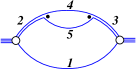
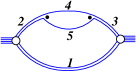
Figure 2: (Color online) Static and kinetic rule for averaging SAWs.

As visualized in Fig. (2), static and kinetic averaging yields different results. The static rule gives $L^{(\text{st})}=(s_{1}+s_{4}+s_{5})/3+2(s_{2}+s_{3})/3$, whereas the kinetic rule produces $L^{(\text{kin})}=(s_{1}+s_{2}+s_{3})/2+(s_{4}+s_{5})/4$. The remaining steps in calculating the diagram essentially textbook matter Am84_ZiJu96 . It turns out, that the static rule does not lead to a renormalizable theory. The reason is easily shown. In the $2$-loop calculation of our example diagram, the non-primitive divergencies arising from the sub-integrations of the $1$-loop self-energy insertion must be cancelled through the counter-terms introduced by the renormalization of this $1$-loop insertion. However, the weights of $L^{(\text{st})}$ are not in conformity with the weights arising in the corresponding $1$-loop diagram with the counterterm insertion: crunching the insertion to a point (corresponding to $s_{4}+s_{5}\rightarrow 0$) leads to $L^{(\text{st})}=s_{1}/3+2(s_{2}+s_{3})/3$ in contrast to $L^{(\text{kin})}=s_{1}/2+(s_{2}+s_{3})/2$, which is equal to $L$ of the $1$-loop self-energy diagram with a point insertion. Hence, only the weighting according to the kinetic rule works correctly in that it leads to a cancellation of non-primitive divergencies by one-loop counterterms. Thus, the static rule has to be rejected on grounds of renormalizability.

Besides revealing the imperative of kinetic averaging, this theory yields two-loop results for the SAW exponents $\nu_{SAW}$ and $\nu_{\text{max}}$, which previously have been calculated (correctly) only to one-loop order MeHa89 ; Ha87 , and the family $\nu^{(\alpha)}$, which is entirely new:

$$\nu_{\mathrm{\max}} =\frac{1}{2}+\frac{\varepsilon}{168}+\Big{[}\frac{5365}{16464}+\frac{15}{28}\Big{(}\ln 2-\frac{69}{70}\ln 3\Big{)}\Big{]}\Big{(}\frac{\varepsilon}{6}\Big{)}^{2}$$

$$\qquad+O(\varepsilon^{3})$$ (7)

$$\nu^{(\alpha)} =\frac{1}{2}+\Big{(}\frac{5}{2}-\frac{3}{2^{\alpha}}\Big{)}\frac{\varepsilon}{42}+\Big{(}\frac{589}{21}-\frac{397}{14\cdot 2^{\alpha}}+\frac{9}{4^{\alpha}}\Big{)}\Big{(}\frac{\varepsilon}{42}\Big{)}^{2}$$

$$\qquad+O(\varepsilon^{3})\,,$$ (8)

where $\varepsilon=6-d$. $\nu_{\mathrm{SAW}}$ is given by $\nu_{\mathrm{SAW}}=\nu^{(1)}$. Our result for $\nu_{\mathrm{SAW}}$ is compared to the available numerical estimates, to our result for the longest SAW, and to the well known exponent $\nu_{\mathrm{\min}}$ for the shortest SAW Ja85 ; JaStOe99 ; JaSt00 in Fig. (3). The following points are worth noting: (i) $\nu^{(\alpha)}$ does not depend on $\alpha$ in a linear or affine fashion which implies that SAWs on percolation clusters are mulitfractal. (ii) $\nu^{(\alpha)}$ is in absolute agreement with the well known results for $D_{bb}$ and $\nu$ in the cases $\alpha=0$ and $\infty$, respectively. (iii) $\nu_{\mathrm{\min}}$ and $\nu_{\mathrm{\max}}$ are not related to the family $\nu^{(\alpha)}$. (iv) the theory is renormalizable for arbitrary $\alpha$ if and only if kinetic averaging is used.

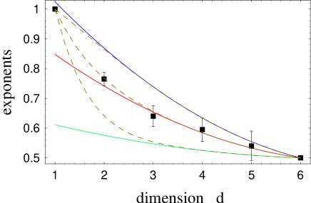
Figure 3: (Color online) The $\varepsilon$-expansions of the exponents $\nu_{\mathrm{min}}$ (blue upper curve), $\nu_{\mathrm{SAW}}$ (red middle curve), and $\nu_{\mathrm{max}}$ (green lower curve). Possible extrapolations at low dimensions $d$ are shown by broken lines. The squares with error bars symbolize numerical results for $\nu_{\mathrm{SAW}}$ as compiled in Chak05 .

As mentioned above, the usual framework to study average SAWs on percolation clusters is the MH model as described by the Hamiltonian

$$\mathcal{H}=\int d^{d}x\,\Big{\{}\sum_{k}\Psi_{k}\bigl{(}r_{k}-\nabla^{2}\bigr{)}\Psi_{k}+\frac{g}{6}\Psi^{3}\Big{\}}\,.$$ (9)

Here, $\Psi_{k}=\{\Psi_{k;\alpha_{1},\ldots\alpha_{k}}^{\;\;\;\;i_{1},\ldots i_{k}}(\mathbf{x})\}$, $1\leq k\leq n$ is an order parameter field conjugate to a $n$-fold replicated $m$-component Heisenberg spin with vector-indices $i_{l}$ running from $1$ to $m$ and replica indices $\alpha_{l}\in\{1,\ldots,n\}$ ordered so that $\alpha_{1}<\cdots<\alpha_{k}$. The $n$ replicas transform according to $n$ different irreducible representations of the direct product of the symmetric group $S_{n}$ and the orthogonal (rotation) group $SO(m)$. $r_{k}=\sum_{l}w_{l}k^{l}$, and $\Psi^{3}$ is a symbolic notation for the sum of the products of three $\Psi_{k}$ fields. Only those cubic terms are allowed for which all pairs $(i,\alpha)$ appear exactly twice. In this model, one can extract $\nu_{\mathrm{SAW}}$ from the renormalization of the relevant control parameter $w_{1}$ upon taking the replica limit $n\to 0$. The MH Hamiltonian (9) is non-renormalizable as it stands. One difficulty, that has been pointed out by Le Doussal and Machta DoMa91 several years ago, is that the critical values {$r_{k}^{c}\}$ of the control parameters are different for different $k$, i.e., the model is highly multicritical. A second problem, that to our knowledge has not been discussed hitherto, is that the order parameter fields $\Psi_{k}$ for different $k$ belong to different irreducible tensor-representations of underlying symmetry group, $S_{n}\times SO(m)$, see above. Hence, strictly speaking, one needs independent coupling constants $g_{k,k^{\prime},k^{\prime\prime}}$ for each product $\Psi_{k}\,\Psi_{k^{\prime}}\,\Psi_{k^{\prime\prime}}$ [note that this is (i) not implemented in the original MH Hamiltonian (9) and (ii) different in the Harris model], and the fields $\Psi_{k}$ need $k$-dependent renormalization factors footnote . Recently, these difficulties caused the failure of a two-loop calculation of $\nu_{SAW}$ by von Ferber et al. FeBlFoHo04 .

As far as its application to the average SAW is concerned, the renormalizability of the MH model can be rescued by a specific interpretation of the replica limit which has close ties to kinetic averaging. Our analysis of the MH model (details will be given elsewhere JaSt06 ) led to the following key findings: If the replica limit is taken after all summations over all possible arrangements of internal replica indices of a diagram, then the MH model reproduces static averaging and, as demonstrated above, is not renormalizable. If, however, the replica limit is taken, in the spirit of Ref. Ha83b , as early as possible, i.e., loop after loop, or at least for each renormalization part, then the MH model reproduces kinetic averaging. This is the only interpretation of replica limit of the MH-model that leads to a renormalizable theory of SAWs in disordered media. With this interpretation, the MH model, in particular, produces the same result for $\nu_{\text{SAW}}$ as our real-world interpretation and thereby provides an important consistency check for the validity of the application of the latter to SAWs.

Closing, we would like to emphasize that our renormalization group arguments are, although certainly well founded, not rigorous in the sense of a mathematical proof since they rely on our real world interpretation of Feynman diagrams. This interpretation thrives on analogy and there exist to date no rigorous mathematical arguments on how far its validity extends. However, given all its successes in the past, we would be surprised if it failed in describing SAWs on percolation clusters. The well known MH model, when interpreted carefully, corroborates the imperative of kinetic averaging and confirms our two-loop result for $\nu_{\text{SAW}}$.

References

- (1) Statistics of Linear Polymers in Disordered Media, edited by B.K. Chakrabarti, (Elsevier, Amsterdam, 2005).
- (2) Y. Meir and A.B. Harris, Phys. Rev. Lett. 63, 2819 (1989).
- (3) P. Le Doussal and J. Machta, J. Stat. Phys. 64, 541 (1991).
- (4) C. von Ferber, V. Blavats’ka, R. Folk, and Yu. Holovatch, Phys. Rev. E 70, 035104(R) (2004), and in Chak05 .
- (5) L. Peliti, J. Phys. (Paris) Lett. 45, L925 (1984); K. Kremer and J. Lyklema, Phys. Rev. Lett. 55, 2091 (1985); L. Pietronero, Phys. Rev. Lett. 55, 2025 (1985).
- (6) S.W. Kenkel and J.P. Straley, Phys. Rev. Lett. 49 , 767 (1982); J.P. Straley and S.W. Kenkel, Phys. Rev. B 29, 6299 (1984).
- (7) A.B. Harris, Phys. Rev. B 35, 5056 (1987).
- (8) R. Blumenfeld and A. Aharony, J. Phys. A 18, L443 (1985); R. Blumenfeld, Y. Meir, A.B. Harris and A. Aharony, J. Phys. A 19, L791 (1986).
- (9) O. Stenull, H.K. Janssen, and K. Oerding, Phys. Rev. E 59, 4919 (1999); H.K. Janssen, O. Stenull, and K. Oerding, Phys. Rev. E 59, R6239 (1999).
- (10) H.K. Janssen and O. Stenull, Phys. Rev. E 61, 4821 (2000).
- (11) O. Stenull, Renormalized Field Theory of Random Resistor Networks, Ph.D. thesis, Universität Düsseldorf, (Shaker, Aachen, 2000).
- (12) O. Stenull and H.K. Janssen, Europhys. Lett. 51, 539 (2000); Phys. Rev. E 63, 036103 (2001).
- (13) H.K. Janssen, Z. Phys B: Condens. Matter 58, 311 (1985); H.K. Janssen and U.C. Täuber, Ann. Phys. (N.Y.) 315, 147 (2005).
- (14) See, e.g., D.J. Amit, Field Theory, the Renormalization Group, and Critical Phenomena (World Scientific, Singapore, 1984); J. Zinn-Justin, Quantum Field Theory and Critical Phenomena (Clarendon, Oxford, 1996).
- (15) It is not possible to construct from the -fold replicated -vector model a simpler model where the order parameter fields for all belong to one and the same irreducible representation of some higher symmetry group. This is in contrast to the -fold replicated -state Potts model that combines to the -state Potts-model, where all fields belong to the same irreducible representation of . Therefore, in the -fold replicated -state Potts model, one gets away with only one coupling parameter and a unique (but -dependent) renormalization factor for all fields.
- (16) A.B. Harris, Phys. Rev. B 28, 2614 (1983).
- (17) H.K. Janssen and O. Stenull, forthcoming paper.