Intrinsic dephasing in one dimensional ultracold atom interferometers

Abstract

Quantum phase fluctuations play a crucial role in low dimensional systems. In particular they prevent true long range phase order from forming in one dimensional condensates, even at zero temperature. Nevertheless, by dynamically splitting the condensate into two parallel decoupled tubes, a macroscopic relative phase, can be imposed on the system. This kind of setup has been proposed as a matter wave interferometer, which relies on the interference between the displaced condensates as a measure of the relative phase between themprentiss ; jorg . Here we show how the quantum phase fluctuations, which are so effective in equilibrium, act to destroy the macroscopic relative phase that was imposed as a non equilibrium initial condition of the interferometer. We show that the phase coherence between the two condensates decays exponentially with a dephasing time that depends on intrinsic parameters: the dimensionless interaction strength, sound velocity and density. Interestingly, at low temperatures the dephasing time is almost independent of temperature. At temperatures higher than a crossover scale $T^{\star}$ dephasing gains significant temperature dependance. In contrast to the usual phase diffusion in three dimensional trapsdiffusion , which is essentially an effect of confinement, the dephasing due to fluctuations in one dimension is a bulk effect that survives the thermodynamic limit.

I Introduction

The existence of a macroscopic phase facilitates observation of interference phenomena in Bose-Einstein condensates (BEC). For example, an interference pattern involving a macroscopic number of particles arises when a pair of condensates is let to expand freely until the two clouds spatially overlap. Since the pioneering experiment by Andrews et alketterle , which demonstrated this effect, it has been a long standing goal to construct matter wave interferometers based on ultra cold atomic gases. Such devices have promising applications in precision measurementkasevich , and quantum information processingjorgQI , as well as fundamental study of correlated quantum matter. The key requirement for interferometric measurement is deterministic control over the phase difference between the two condensates. That is, the relative phase must be well defined and evolve with time under the sole influence of the external forces which are the subject of measurement. This requirement was not met for example in the setup of Ref. [ketterle, ], where the two condensates were essentially independent and the relative phase between them was initially undetermined.

One way to initialize a system with a well defined phase is to construct the analogue of a beam splitter whereby a single condensate is dynamically split into two coherent parts, which serve as the two “arms” of the interferometershin ; prentiss ; jorg ; prentiss2 . In recent experiments this was achieved by raising a potential barrier along the axis of a quasi one-dimensional condensatejorg . The split is applied slowly compared to the transverse frequency of the trap, but fast compared to the longitudinal time scales. Thus each atom is transferred in this process to the symmetric superposition between the two traps without significantly changing its longitudinal position. An illustration of the procedure is given in Fig. 1. In repeated experiments the condensates are released from the trap to probe the interference at varying times after the split. Immediately following the split the two condensates are almost perfectly in phase. However repeated measurements at longer times show that the phase distribution becomes gradually broader until it becomes uniformly distributed on the interval $[0,2\pi]$. The accuracy of interferometric measurements is limited by such dephasing.

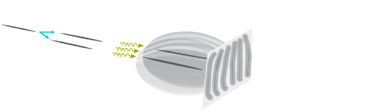
Figure 1: Interferometer setup. At time $t=0$ a single one-dimensional condensate is split into two coherent parts by raising a high potential barrier along the condensate axis. After a wait time $t$ the condensates are released from the trap and let to expand. After a sufficient expansion time the cloud is imaged by a probe beam sent along the condensate axis and the phase of the resulting interference pattern is recorded. This process is repeated many times in order to obtain a phase distribution at a number of different wait times $t$.

In this paper we develop a theory of dephasing in interferometers made of one dimensional Bose gases. We assume that such systems can be well isolated from the noisy environment, so that this source of decoherencebruder is set at bay. Another dephasing mechanism that has been discussed extensively in the context of condensates in double wells is ”quantum phase diffusion”shin ; diffusion ; menotti . The uncertainty in the particle numbers in each well brought about by the split, entails a concomitant uncertainty in the chemical potential difference, which leads to broadening of the global relative phase on a time scale of $\tau_{D}\sim\hbar\sqrt{N}/\mu$. Here $N$ is the total particle number and $\mu$ is the chemical potential. Note that this is essentially a finite size effect. $\tau_{D}$ diverges in the proper thermodynamic limit in which the trap frequency is taken to zero while the density is kept constant. Here we show that dephasing in quasi one dimensional systems is dominated by a new mechanism that involves quantum fluctuations of the local relative phase field rather than the global phase difference between the condensates. In contrast to the usual phase diffusion this is a bulk mechanism that survives the thermodynamic limit. Indeed, it is well known that in one dimensional liquids quantum phase fluctuations are extremely effective and prevent the formation of long range order. Here we show how these fluctuations destroy long range order in the relative phase, that was imposed on the system by the initial conditions. We account for the phase fluctuations using a quantum hydrodynamic description of the Bose liquids haldane . The phase coherence between the condensates is then shown to decay exponentially in time. The dephasing time we obtain is a simple function of intrinsic parameters: the dimensionless interaction strength, the density, and the sound velocity. These predictions are verified and extended to finite temperatures, using direct simulation of the dynamics in the microscopic hamiltonian. The results are also compared to the dephasing time measured in Ref. [jorg, ], and are found to be in quantitative agreement.

It is interesting to point out the essential difference between the problem we consider and dephasing of single particle interference effects as considered for example in mesoscopic electron systems. As in our problem, phase coherence in mesoscopic systems can be defined by an interferometric measurementheiblum . In a Fabry-Perot setup, oscillations of the conductivity as a function of applied Aharonov-Bohm flux vanish exponentially with system size, thereby defining a characteristic dephasing length. Because what is measured is ultimately the DC conductivity, the problem may be recast in terms of linear response theorystern . By contrast, dynamic splitting of the condensate in the ultra-cold atom interferometer takes the system far from equilibrium and the question of phase coherence is then essentially one of quantum dynamics. The system is prepared in an initial state determined by the ground state of a single condensate, which then evolves under the influence of a completely different hamiltonian, that of the split system. Dephasing, from this point of view, is the process that takes the system to a new steady (or quasi-steady) state.

II Hydrodynamic theory

We start our analysis by considering the hydrodynamic theory that describes low energy properties of one dimensional Bose liquidshaldane . The hydrodynamic hamiltonian for a pair of decoupled condensates is that of two decoupled Luttinger liquids (we set $\hbar=1$ throughout)

$$H={c\over 2}\sum_{{\alpha}=1}^{2}\int dx\left[{K\over\pi}(\nabla{\varphi}_{\alpha})^{2}+{\pi\over K}\Pi_{\alpha}^{2}\right],$$ (1)

where $c$ is the sound velocity and K is the Luttinger parameter that determines the decay of correlations at long distance. $\Pi_{\alpha}$ is the density fluctuation operator conjugate to the phase ${\varphi}_{\alpha}$. The smooth component of the Bose field operator is given by $\psi_{\alpha}\approx\sqrt{\rho}\exp(i{\varphi}_{\alpha})$, where $\rho$ is the average densityhaldane .

The operator corresponding to the interference signal between the two condensates is given bypad :

$$A\approx\rho\int_{0}^{L}dx~{}e^{i({\varphi}_{1}(x)-{\varphi}_{2}(x))},$$ (2)

where $L$ is the imaging length. For a pair of decoupled condensates at equilibrium, ${\langle A\rangle}=0$ while ${\langle A^{2}\rangle}>0$pad . Therefore the interference pattern displayed in repeated experiments has a finite amplitude but its phase is completely random. On the contrary, in this work we consider a pair of condensates that are prepared out of equilibrium, with a well defined relative phase. In this case ${\langle A\rangle}$ is expected to be non vanishing at the time of the split and decay in time as the fluctuation in relative phase grows.

Calculation of the time evolution of ${\langle A\rangle}$ is greatly simplified by the fact that the hydrodynamic theory is quadratic. In particular, this allows decoupling in the hamiltonian of ”center of mass” and relative phase fields ${\varphi}_{+}=({\varphi}_{1}+{\varphi}_{2})/2$ and ${\varphi}_{-}={\varphi}_{1}-{\varphi}_{2}$. In other words, the hamiltonian can be rewritten as a sum of two commuting harmonic terms $H=H_{+}({\varphi}_{+},\Pi_{+})+H_{-}({\varphi}_{-},\Pi_{-})$, where $\Pi_{\pm}$ are the conjugate momenta of ${\varphi}_{\pm}$. Moreover, the splitting process described above ensures that the initial state may be factorized as $\Psi[{\varphi}_{+},{\varphi}_{-}]=\Psi_{+}[{\varphi}_{+}]\times\Psi_{-}[{\varphi}_{-}]$. Because during the split all atoms are simply transferred to the symmetric superposition without changing their axial state, the wave function $\Psi_{+}[{\varphi}_{+}]$ is identical to the wave function of the single condensate before the split. If this condensate is at finite temperature $\Psi_{+}$ is replaced by the appropriate density matrix. On the other hand $\Psi_{-}$ is determined by the splitting process and will generally be strongly localized around ${\varphi}_{-}(x)=0$. In fact we can find the approximate form of this wavefunction, which will be an important input for the time dependant calculation.

Consider a region of size $\xi_{h}$, which is the length scale on which the hydrodynamic variables are defined. Let $n_{1}$ and $n_{2}$ be the operators corresponding to the particle number in each of the condensates within this region. The splitting process delocalizes the particles between the two condensates, resulting in a roughly gaussian distribution of the relative particle number $n_{-}=(n_{1}-n_{2})/2$, with an uncertainty of order $\sqrt{{\langle n_{1}+n_{2}\rangle}/4}=\sqrt{\rho\xi_{h}/2}$. The phase ${\varphi}_{-}$ defined on this grain in the hydrodynamic theory is canonically conjugate to $n_{-}$. Therefore the wave function in the phase representation is approximately gaussian withsqueezed ${\langle{\varphi}(x){\varphi}(x^{\prime})\rangle}\approx{\delta}(x-x^{\prime})/(2\rho)$. That is

$$\Psi_{-}[{\varphi}_{-}]\propto e^{-{1\over 2}\rho\int dx|{\varphi}(x)|^{2}}=e^{-{1\over 2}\rho\sum_{q}|{\varphi}_{q}|^{2}}.$$ (3)

From here on we drop the subscript (-) where no ambiguity may arise.

We are now ready to compute ${\langle A\rangle}$ which depends only on ${\varphi}_{-}$. The wave-function $\Psi_{-}[{\varphi}_{-}]$ evolves in time under the influence of the harmonic hamiltonian

$$H_{-}={c\over 2}\sum_{q}\left({2\pi\over K}|\Pi_{q}|^{2}+{Kq^{2}\over 2\pi}|{\varphi}_{q}|^{2}\right).$$ (4)

The wavefunction remains gaussian at all times:

$$\Psi_{-}[{\varphi},{\varphi}^{\star}]=\prod_{q}\left({1\over 2\pi W_{q}}\right)^{1/4}~{}e^{-{|{\varphi}_{q}|^{2}\over 4W_{q}}}e^{-i{\eta}_{q}}$$ (5)

where ${\eta}_{q}({\varphi}_{q},{\varphi}^{\star}_{q},t)$ is a pure phase and

$$W_{q}(t)={\langle|{\varphi}_{q}|^{2}\rangle}={1\over 2\rho}\cos^{2}(cqt)+{2\pi^{2}\rho\sin^{2}(cqt)\over K^{2}q^{2}}.$$ (6)

The expectation value ${\langle A\rangle}={\cal A}$ in the gaussian wave function (5) is given by

$${\cal A}(t)=\rho{\langle e^{i{\varphi}(x)}\rangle}=\rho e^{-{1\over 2L}\sum_{q}{\langle|{\varphi}_{q}|^{2}\rangle}}=\rho e^{-g(t)}.$$ (7)

In the thermodynamic limit ($L\to\infty$) the summation in (7) can be converted to an integral to obtain:

$$g(t) \approx {1\over 2\pi}\int_{0}^{\pi/\xi_{h}}dq\left[{1\over 2\rho}\cos^{2}(cqt)+{2\pi^{2}\rho\sin^{2}(cqt)\over K^{2}q^{2}}\right]$$ (8)

$$\approx g_{0}+{\rho ct\over 2(K/\pi)^{2}}.$$

The last equality is valid at times $t>\xi_{h}/c$, when the integrals become independent of the high momentum cutoff. In addition we require that the particle number in a healing length $\xi_{h}$ is large, i.e. $\rho\xi_{h}\gg 1$, this is always satisfied at weak coupling $K\gg 1$. Thus we find that the phase coherence decays exponentially:

$${\cal A}(t)={\cal A}_{0}e^{-t/\tau}$$ (9)

with the characteristic time

$$\tau={2\over c\rho}(K/\pi)^{2}.$$ (10)

Note that the dephasing time $\tau$ diverges, as it must, in the non interacting limit ($K\to\infty$ and $c\to 0$). Clearly the initial state induced by the split is an eigenstate of non interacting particles and therefore all observables including the coherence must be time independent in this limit.

For a finite system, the discreteness of the sum in (7) must be taken into account at times $t\gg L/c$. In such a case, the dominant contribution to $g(t)$ arises from the $q=0$ term. This term yields a ballistic broadening of the phase ${\langle{\varphi}^{2}_{q=0}\rangle}\propto t^{2}$, which results in a gaussian decay of the coherence: ${\cal A}(t)={\cal A}_{0}\exp(-t^{2}/\tau_{L}^{2})$ where $\tau_{L}=\sqrt{\tau L/2c}$.

It is interesting to note that one can also express the time scale associated with the finite size as $\tau_{L}\propto\sqrt{N}/\mu$. Written in this way, it is clear that the gaussian term is just the ”quantum phase diffusion” discussed in the context of double well systemsshin ; diffusion . It stems from the uncertainty relation between the uniform component of the relative phase and the difference in total particle numbers between the wells. The uniform component of the interaction, which drives the ballistic broadening of ${\varphi}_{q=0}$ scales like $1/L$, making the gaussian term irrelevant in large systems. By contrast, the exponential dephasing due to the internal modes is length independent. The fact that these modes produce exponential dephasing is special to one dimensional interferometers. A similar analysis of two parallel planar condensates yields logarithmic divergence in (8), which implies power law decay of the coherence as ${\cal A}\propto(\xi_{h}/ct)^{\alpha}$. We note that in this case $K$ is not dimensionless. The power ${\alpha}$ is non universal and depends on the short distance cutoff. In three dimensions on the other hand the only contribution to dephasing is the usual phase diffusion due to finite size and there is no bulk contribution.

It is striking that the hydrodynamic theory developed in this section predicts a dephasing time which is independent of temperature. Temperature enters the initial condition only through the density matrix for the symmetric degrees of freedom, whereas the phase coherence between the condensates depends on the evolution of the relative phase. Because the symmetric and antisymmetric fields are completely decoupled within the harmonic theory, the temperature associated with the symmetric degrees of freedom does not affect the dephasing. However, it is clear that the full microscopic hamiltonian contains anharmonic terms that do couple those degrees of freedom. At equilibrium the non linear terms are irrelevant (in the renormalization group sense) and do not affect the asymptotic long wavelength low energy correlations. However it is natural to question the validity of the hydrodynamic description for computing time dependent properties. In particular, here the system is prepared out of equilibrium in a state with extensive energy relative to the ground state. Then it is a priori unclear that the low energy correlations given by the hydrodynamic theory are sufficient to describe the dynamics. In the next section we shall test the predictions of the hydrodynamic theory and obtain temperature dependent corrections to the dephasing by computing the dynamics within a microscopic model of the twin condensates.

III Numerical results

For the purpose of numerical calculations we shall consider a lattice hamiltonian, the Bose-Hubbard model on twin chains

$$H=-J\sum_{i}\sum_{{\alpha}=1}^{2}(b^{\dagger}_{{\alpha}i}b{{}^{\vphantom{\dagger}}}_{{\alpha}i+1}+H.c.)+{U\over 2}\sum_{{\alpha}i}n_{{\alpha}i}(n_{{\alpha}i}-1).$$ (11)

Here $b^{\dagger}_{{\alpha}i}$ creates a Boson on site $i$ of chain ${\alpha}$. The model (11) can also describe continuum systems, such as the one in Ref. [jorg, ], if the average site occupation $\bar{n}={\langle n_{i}\rangle}$ is much less than unity.

As mentioned above, we are interested in the time evolution of the expectation value ${\cal A}(t)=\sum_{i}{\langle b^{\dagger}_{1i}(t)b{{}^{\vphantom{\dagger}}}_{2i}(t)\rangle}$. The average is taken over the wave function or density matrix at the time of the split. We will calculate ${\cal A}(t)$ using a semiclassical approach called the truncated Wigner approximation (TWA, cf. Ref. [polkovnikov, ]). Let us first briefly review the strictly classical approximation to the dynamics. The usual procedure is to write the Heisenberg equations of motion for $b{{}^{\vphantom{\dagger}}}_{i}$ and $b^{\dagger}_{i}$ and then replace these operators by complex classical fields $\psi_{i}$ and $\psi^{\star}_{i}$. This leads to the lattice Gross-Pitaevskii (GP) equations

$$i{d\psi_{{\alpha},i}\over dt}=-J(\psi_{{\alpha},i-1}+\psi_{{\alpha},i+1})+U|\psi_{{\alpha},i}|^{2}\psi_{{\alpha},i}.$$ (12)

Given the initial condition $\psi_{{\alpha},i}(0)$ one can integrate the GP equations to find the value of the fields at any time $t$ and obtain ${\cal A}_{cl}(t)=\sum_{i}\psi^{\star}_{1i}(t)\psi_{2i}(t)$. If the split is fully coherent $\psi_{1i}(0)=\psi_{2i}(0)$. Since the evolution in the two chains is described by identical equations, this equality persists to all subsequent times. Thus in the absence of external noise sources, the classical dynamics cannot account for dephasing. By contrast, quantum fluctuations provide an intrinsic dephasing mechanism.

Quantum corrections modify the dynamics in two ways. First, they introduce ”quantum noise” to the initial conditions. The fields $\psi_{{\alpha}i}$ and $\psi^{\star}_{{\alpha}i}$ originate from non commuting quantum operators $b{{}^{\vphantom{\dagger}}}_{{\alpha}i}$ and $b^{\dagger}_{{\alpha}i}$ which cannot be determined simultaneously. Therefore the unique classical initial condition should be replaced by an ensemble of initial conditions characterized by a quantum distribution. Second, the classical trajectories determined by (12) are supplemented by additional quantum paths.

It can be shown that the leading quantum correction to the dynamics enters through the initial conditionspolkovnikov . The essence of TWA is to integrate the GP equations starting from an ensemble of initial conditions, which are given quantum weights derived from the initial density matrix. Thus within this approximation:

$${\cal A}(t)=\int{\mathcal{D}}\{\psi^{\star}_{j{\alpha}},\psi_{j{\alpha}}\}_{0}\rho_{\mbox{\tiny W}}(\{\psi^{\star}_{j{\alpha}},\psi_{j{\alpha}}\}_{0}){\cal A}_{cl}(t).$$ (13)

Here

$$\rho_{\mbox{\tiny W}}(\psi^{\star},\psi) \equiv \int d{\eta}^{\star}d{\eta}{\,\langle\,\psi-{{\eta}\over 2}\,|\,}\rho_{0}{\,|\,\psi+{{\eta}\over 2}\,\rangle\,}$$ (14)

$$\times e^{-|\psi|^{2}-{1\over 4}|{\eta}|^{2}}e^{{1\over 2}({\eta}^{\star}\psi-{\eta}\psi^{\star})},$$

is the Wigner representation of the initial density matrix of the system and ${\,|\,\psi\,\rangle\,}$ denotes a coherent state with eigenvalue $\psi$ of the boson annihilation operator. We note that $\rho_{\mbox{\tiny W}}$ should not be thought of as a probability distribution, because in general it can assume negative values.

The main difficulty in applying the recipe (13) to compute ${\cal A}(t)$ is the need to find the Wigner distribution of the split condensate at the time of the split. To overcome this problem we use the following procedure. Rather than tackling a split interacting system we start the calculation from a single non-interacting condensate, where we have an exact expression for $\rho_{\mbox{\tiny W}}$polkovnikov . The evolution of the Wigner distribution from a non-interacting system to an interacting one is done using the TWA by slowly increasing the interaction constant, $U$, from zero to the desired value (see footnote [footnote, ]). The heating induced by the time dependant hamiltonian is controlled by the rate at which $U$ is increased. The next step is the split of the condensate. It involves the doubling of the degrees of freedom at each site. Because of the way the split is carried out, the field $\psi_{i}$ of the single condensate is simply copied to the symmetric field $\psi_{+,i}\equiv(\psi_{1i}+\psi_{2i})/\sqrt{2}$. The new degree of freedom $\psi_{-,i}$ is chosen at this point from a Wigner distribution

$$\rho^{(-)}_{\mbox{\tiny W}}(\{\psi^{\star}_{-},\psi_{-}\}_{0})=\prod_{i}\left({2\over\pi}\right)e^{-2|\psi_{-,i}|^{2}}$$ (15)

which corresponds to the vacuum of the boson $b_{-,i}=(b_{1i}-b_{2i})/\sqrt{2}$. The calculation is continued using the dynamics of the twin condensates.

Figure 2: Decay of the coherence calculated with the truncated Wigner approximation for $U=1$, $J=1$ and ${\bar{n}}=7.5$ compared to the result of the hydrodynamic theory (dots). The time axis is scaled to the hydrodynamic dephasing time $\tau_{0}$ (10). Lines correspond to different initial temperatures parameterized by the correlation length $\xi_{T}$ that existed before the split.

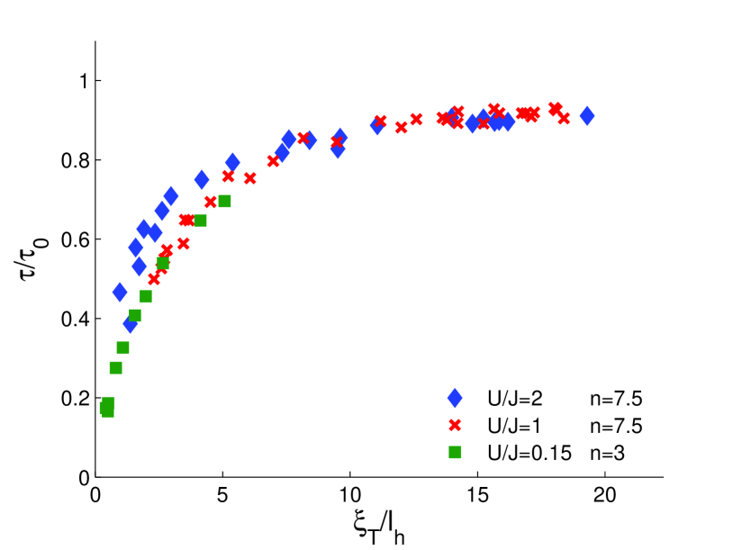
Figure 3: Dephasing time $\tau$ as a function of the thermal correlation length, which is a measure of the inverse temperature before the split. Data is taken in different regimes of microscopic parameters. All data is seen to collapse on approximately the same curve when the dephasing time is scaled to the theoretical time scale (10) and the thermal correlation length scaled by $l_{h}$ (see text).

The condensate (prior to the split) is prepared at various temperatures using two different methods: (i) By initializing the non interacting condensate in a finite temperature density matrix. (ii) By varying the rate by which the interactions are switched on to induce a controlled amount of heating. The temperature of the condensate before the split is parameterized by measuring the correlation length $\xi_{T}\propto 1/T$ associated with the decay of the correlation function ${\langle b^{\dagger}_{i}b{{}^{\vphantom{\dagger}}}_{i+r}\rangle}$. We verified that the final result for ${\cal A}(t)$ depends only on $\xi_{T}$ and not on the method used to achieve finite temperature.

Finally, in order to compare the numerical results to the prediction of the hydrodynamic theory we use the fact that at weak coupling there are simple relations between the parameters of the microscopic model (11) and those of the hydrodynamic theory (1)cazalilla . In particular the value of the Luttinger parameter is given by $K\approx\pi\sqrt{2J{\bar{n}}/U}$, and the sound velocity is $c=\sqrt{2J{\bar{n}}U}$. The short distance cutoff of the hydrodynamic theory may also be extracted from (11), by finding the length over which amplitude fluctuations decay. It is given by footnote_xi $l_{h}=\sqrt{2}\xi_{h}\approx a\sqrt{4J/U{\bar{n}}}$. Increasing $\bar{n}$ decreases this length scale until it reaches its lower bound which is one lattice constant $a$. When $l_{h}\gg a$ the model (11) in effect describes a continuum system, while for a large site occupancy $l_{h}\to a$ it describes a lattice of coupled condensates. We perform simulations in both regimes. The continuum regime is much more demanding computationally in the sense that attaining a given thermal correlation length in this regime requires a much slower activation rate of the interaction. This limited the temperature range we could study in the continuum regime.

The numerical results are summarized in Fig. 2 and Fig. 3. The dephasing time, $\tau$, is extracted by fitting ${\cal A}(t)$ to Eq. (9). At low temperatures, $\tau$ is in good agreement with the hydrodynamic result (10) and shows very weak temperature dependence. On the other hand above a crossover temperature $T^{\star}$, the dephasing time gains significant temperature dependence. The crossover scale is set by the condition $\xi_{T^{\star}}\sim l_{h}$. This is not surprising, given that the hydrodynamic theory is expected to break down when correlations decay over a length scale shorter than its short distance cutoff. The agreement between the numerical results and the hydrodynamic theory at low temperatures is highly non-trivial in view of the fact that the two approaches are based on entirely different approximations. Most importantly, the temperature independent result (10) relied on the decoupling of symmetric and antisymmetric degrees of freedom within the harmonic theory (1). Such decoupling does not exist in the microscopic model (11) nor in the TWA dynamics. In the next section we shall compare the results of the hydrodynamic theory to experimental data.

IV Comparison with experiments

The dephasing time (10) is written in terms of parameters of the hydrodynamic theory. In order to compare with experiments we have to translate these parameters to numbers that are relevant to a specific experimental situation. For this purpose we will consider the setup of the experiments described in Ref. [jorg, ].

This system consists of bosons with contact interactions parameterized by a dimensionless interaction strength $\gamma$. At weak coupling, $\gamma\ll 1$, the following relations holdcazalilla : $K=\pi/\sqrt{\gamma}$ and $c=\hbar(\rho/M)\sqrt{\gamma}$, where $M$ is the mass of an atom. Substituting these into (10) we obtain:

$$\tau=\left({2M\over\hbar\rho^{2}}\right){1\over\gamma^{3/2}}.$$ (16)

Now consider a one dimensional tube geometry with transverse trap frequency ${\omega}_{\perp}$. If the oscillator length $l_{\perp}$ is much larger than the $s-wave$ scattering length $a_{s}$, as is the case in Ref. [jorg, ], we can use the approximate expression $\gamma\approx 2M{\omega}_{\perp}a_{s}/\hbar\rho$  olshanii ; cazalilla . This allows us to write the dephasing time using parameters easily determined in the experiment:

$$\tau=\sqrt{\hbar\over 2M\rho}\left({1\over{\omega}_{\perp}a_{s}}\right)^{3/2}$$ (17)

Note that $\rho$ is the density per condensate in the split system, that is half the density of the initial condensate.

Taking the scattering length of rubidium-87 atoms $a_{s}=105a_{0}$, the transverse trap frequency ${\omega}_{\perp}=2\pi\times 2.1~{}kHz$ and density of about $50$ atoms per micronjorg-private , we obtain a dephasing time $\tau\approx 4.3$ms. To estimate the dephasing time in the experimentjorg we use the data for the phase broadening assuming a von Mises distribution of the phase ($f({\theta})=\exp(\kappa\cos{\theta})/2\pi I_{0}(\kappa)$). This gives approximately $2$ms, slightly shorter than our theoretical estimate. We note that data points marked with squares in Fig. 3 correspond to parameters relevant to the experiment. Unfortunately the temperature in that experiment is not known to a good accuracy. In the future it would be interesting to look for the universal temperature dependence implied by the numerical results.

V Discussion and Conclusions

It is well known that quantum fluctuations prevent long range phase order from forming in one-dimensional Bose liquids. This phenomenon is most conveniently described within the framework of the Luttinger liquid or hydrodynamic theory. Here we used this framework in a non equilibrium situation to show how quantum fluctuations destroy long range order that was imposed on the system as an initial condition. The outcome is a simple formula describing exponential decay of phase coherence in interferometers made of one-dimensional condensates. The dephasing time found in this way provides a fundamental limit on the accuracy of such interferometers. We did not discuss the situation in which the interferometer is prepared in a number squeezed initial state. Such an initial condition would slow the usual phase diffusion processmenotti ; prentiss2 and is expected to similarly affect the bulk mechanism discussed in this paper.

Interestingly the dephasing time measured in Ref. [jorg, ] is only slightly shorter than the prediction of the hydrodynamic theory. We therefore conclude that quantum phase fluctuations were probably a dominant dephasing mechanism in that experiment.

The validity of the Luttinger liquid framework out of equilibrium is not ensured a priori. We therefore test its predictions against numerical simulations of the microscopic model using the Truncated Wigner approximation. At low temperatures, the simulation results were essentially temperature independent and in good agreement with the hydrodynamic theory. On the other hand at temperatures above a crossover scale set by the healing length, the dephasing time displayed considerable temperature dependence. Indeed the Luttinger liquid theory is expected to break down above this temperature scale.

Phase fluctuations are expected to be weaker at higher dimensions. For example three dimensional condensates can support long range order even at finite temperatures. In this case the long range order in the relative phase imposed as an initial condition of the interferometer is resistant to the phase fluctuations. The situation with planar condensates is more delicate. two dimensional systems can in principle sustain long range order at equilibrium at zero temperature. However the initial condition of the interferometer drives the system out of equilibrium. The hydrodynamic theory yields power law dephasing in this case. However the power is non universal and further work is needed to test the validity of the hydrodynamic theory.

Finally we would like to point out that the dephasing process considered in this paper is a mechanism that brings the system, from a non equilibrium state imposed by the initial conditions to a new steady state. According to the hydrodynamic theory this steady (or quasi-steady) state is not yet thermal equilibrium. In particular we find that the off diagonal correlations along the condensates are distinctly non thermal at steady stateunpublished . It is an interesting question whether there are processes, much slower than dephasing, that eventually take the system toward thermal equilibrium. This issue can be addressed by experiments. After the phase has randomized, correlations along the condensates can be measured using analysis methods developed in Refs. [pad, ; gadp, ]. Thus, we propose that interferometric experiments can serve as detailed probes to address fundamental questions in non equilibrium quantum dynamics, supplementing measurements of global properties previously used to touch on these issuesweiss .

Acknowladgements. We are grateful to N. Davidson, E. Demler, S. Hofferberth, A. Polkovnikov, J. Schmiedmayer, T. Schumm, and J. H. Thywissen for useful discussions. This work was partially supported by the U.S. Israel BSF and by an Alon fellowship.

References

- (1) Y. Shin, C. Sanner, G.-B. Jo, T. A. Pasquini, M. Saba, W. Ketterle, D. E. Pritchard, M. Vengalattore, and M. Prentiss, Phys. Rev. A 72, 021604 (2005).
- (2) T. Schumm et al, Nature Phys. 1, 57 (2005).
- (3) G.-B. Jo et al, cond-mat/0608585
- (4) F. Sols, Physica (Amsterdam) 194B 196B, 1389 (1994); M. Lewenstein and L. You, Phys. Rev. Lett. 77, 3489 (1996);
- (5) C. Menotti, J. R. Anglin, J. I. Cirac, and P. Zoller, Phys. Rev. A 63, 023601 (2001).
- (6) M. R. Andrews, C. G. Townsend, H. J. Miesner, D. S. Durfee, D. M. Kurn, and W. Ketterle, Science 275, 637 (1997).
- (7) M. A. Kasevich, Science 298, 1363 (2002).
- (8) M. A. Cirone, A. Negretti, T. Calarco, P. Kruger, and J. A. Schmiedmayer, Eur. Phys. J. D 35, 165 171 (2005).
- (9) Y. Shin et al, Phys. Rev. Lett. 92, 050405 (2004)
- (10) C. Schroll, W. Belzig, and C. Bruder, Phys. Rev. A 68, 043618 (2003).
- (11) F. D. M. Haldane, Phys. Rev. Lett. 47, 1840 (1981).
- (12) E. Buks et al, Nature 391, 871 (1998).
- (13) A. Stern, Y. Aharonov, and Y. Imry, Phys. Rev. A 41, 3436(1990)
- (14) A. Polkovnikov, E. Altman, and E. Demler, PNAS 103, 6125 (2006).
- (15) The interferometer can also be prepared in a number squeezed initial state menotti ; prentiss2 . This situation will not be discussed in detail in the present paper.
- (16) A. Polkovnikov, Phys. Rev. A, 68, 033609 (2003); ibid. 68, 053604 (2003).
- (17) The interaction is activated using , where controls the degree of adiabaticity.
- (18) M. A. Cazalilla, J. Phys. B 37, S1-S47 (2004).
- (19) This length scale may be obtained by solving Gross-Pitaevskii boundary problem in which the wave function increases from zero at to its bulk value at . See e.g. C. J. Pethick and H. Smith, ”Bose-Einstein condensation in dilute gases”, p. 162, Cambridge University Press (2002).
- (20) M. Olshanii, Phys. Rev. Lett. 81, 938 (1998).
- (21) R. Bistritzer and E. Altman, unpublished
- (22) V. Gritsev, E. Altman, and E. Demler, and A. Polkovnikov, cond-mat/0602475
- (23) J. Schmiedmayer, private communication
- (24) T. Kinoshita, T. Wenger, and D. S. Weiss, Nature 440, 900 (2006).