Transport of multiple users in complex networks

Abstract

We study the transport properties of model networks such as scale-free and Erdős-Rényi networks as well as a real network. We consider the conductance $G$ between two arbitrarily chosen nodes where each link has the same unit resistance. Our theoretical analysis for scale-free networks predicts a broad range of values of $G$, with a power-law tail distribution $\Phi_{\rm SF}(G)\sim G^{-g_{G}}$, where $g_{G}=2\lambda-1$, and $\lambda$ is the decay exponent for the scale-free network degree distribution. We confirm our predictions by large scale simulations. The power-law tail in $\Phi_{\rm SF}(G)$ leads to large values of $G$, thereby significantly improving the transport in scale-free networks, compared to Erdős-Rényi networks where the tail of the conductivity distribution decays exponentially. We develop a simple physical picture of the transport to account for the results. We study another model for transport, the max-flow model, where conductance is defined as the number of link-independent paths between the two nodes, and find that a similar picture holds. The effects of distance on the value of conductance are considered for both models, and some differences emerge. We then extend our study to the case of multiple sources, where the transport is define between two groups of nodes. We find a fundamental difference between the two forms of flow when considering the quality of the transport with respect to the number of sources, and find an optimal number of sources, or users, for the max-flow case. A qualitative (and partially quantitative) explanation is also given.

1 Introduction

Transport in many random structures is “anomalous,” i.e., fundamentally different from that in regular space [1, 2, 3]. The anomaly is due to the random substrate on which transport is constrained to take place. Random structures are found in many places in the real world, from oil reservoirs to the Internet, making the study of anomalous transport properties a far-reaching field. In this problem, it is paramount to relate the structural properties of the medium with the transport properties.

An important and recent example of random substrates is that of complex networks. Research on this topic has uncovered their importance for real-world problems as diverse as the World Wide Web and the Internet to cellular networks and sexual-partner networks [4]. Networks describe also economic systems such as financial markets and banks systems [5, 6, 7]. Transport of goods and information in such networks is of much interest.

Two distinct models describe the two limiting cases for the structure of the complex networks. The first of these is the classic Erdős-Rényi model of random networks [8], for which sites are connected with a link with probability $p$ and are disconnected (no link) with probability $1-p$ (see Fig. 1(a)). In this case the degree distribution $P(k)$, the probability of a node to have $k$ connections, is a Poisson

$$P(k)=\frac{\left(\overline{k}\right)^{k}e^{-\overline{k}}}{k!},$$ (1)

where $\overline{k}\equiv\sum_{k=1}^{\infty}kP(k)$ is the average degree of the network. Mathematicians discovered critical phenomena through this model. For instance, just as in percolation on lattices, there is a critical value $p=p_{c}$ above which the largest connected component of the network has a mass that scales with the system size $N$, but below $p_{c}$, there are only small clusters of the order of $\log N$. At $p=p_{c}$, the size of the largest cluster is of order of $N^{2/3}$.Another characteristic of an Erdős-Rényi network is its “small-world” property which means that the average distance $d$ (or diameter) between all pairs of nodes of the network scales as $\log N$ [9]. The other model, recently identified as the characterizing topological structure of many real world systems, is the Barabási-Albert scale-free network and its extensions [10, 11, 12], characterized by a scale-free degree distribution:

$$P(k)\sim k^{-\lambda}\qquad[k_{\rm min}\leq k\leq k_{\rm max}],$$ (2)

The cutoff value $k_{\rm min}$ represents the minimum allowed value of $k$ on the network ($k_{\rm min}=2$ here), and $k_{\rm max}\equiv k_{\rm min}N^{1/(\lambda-1)}$, the typical maximum degree of a network with $N$ nodes [13, 14]. The scale-free feature allows a network to have some nodes with a large number of links (“hubs”), unlike the case for the Erdős-Rényi model of random networks [8, 9] (See Fig. 1(b)). Scale-free networks with $\lambda>3$ have $d\sim\log N$, while for $2<\lambda<3$ they are “ultra-small-world” since the diameter scales as $d\sim\log\log N$ [13].

Here we extend our recent study of transport in complex networks [15, 16]. We find that for scale-free networks with $\lambda\geq 2$, transport properties characterized by conductance display a power-law tail distribution that is related to the degree distribution $P(k)$. The origin of this power-law tail is due to pairs of nodes of high degree which have high conductance. Thus, transport in scale-free networks is better because of the presence of large degree nodes (hubs) that carry much of the traffic, whereas Erdős-Rényi networks lack hubs and the transport properties are controlled mainly by the average degree $\overline{k}$ [9, 17]. We present a simple physical picture of the transport properties and test it through simulations. We also study a form of frictionless transport, in which transport is measured by the number of independent paths between source and destination. These later results are in part similar to those in [18]. We test our findings on a real network, a recent map of the Internet. In addition, we study the properties of the transport where several sources and sinks are involved. We find a principal difference between the two forms of transport mentioned above, and find an optimal number of sources in the frictionless case.

The paper is structured as follows. Section 2 concentrates on the numerical calculation of the electrical conductance of networks. In Sec. 3 a simple physical picture gives a theoretical explanation of the results. Section 4 deals with the number of link-independent paths as a form of frictionless transport. In Section 5 we extend the study of frictionless transport to the case of multiple sources. Finally, in Sec. 6 we present the conclusions and summarize the results in a coherent picture.

2 Transport in complex networks

Most of the work done so far regarding complex networks has concentrated on static topological properties or on models for their growth [4, 13, 11, 19]. Transport features have not been extensively studied with the exception of random walks on specific complex networks [20, 21, 22]. Transport properties are important because they contain information about network function [23]. Here we study the electrical conductance $G$ between two nodes $A$ and $B$ of Erdős-Rényi and scale-free networks when a potential difference is imposed between them. We assume that all the links have equal resistances of unit value [24].

We construct the Erdős-Rényi and scale-free model networks in a standard manner [15, 25]. We calculate the conductance $G$ of the network between two nodes $A$ and $B$ using the Kirchhoff method [26], where entering and exiting potentials are fixed to $V_{A}=1$ and $V_{B}=0$.

First, we analyze the probability density function (pdf) $\Phi(G)$ which comes from $\Phi(G)dG$, the probability that two nodes on the network have conductance between $G$ and $G+dG$. To this end, we introduce the cumulative distribution $F(G)\equiv\int_{G}^{\infty}\Phi(G^{\prime})dG^{\prime}$, shown in Fig. 2 for the Erdős-Rényi and scale-free ($\lambda=2.5$ and $\lambda=3.3$, with $k_{\rm min}=2$) cases. We use the notation $\Phi_{\rm SF}(G)$ and $F_{\rm SF}(G)$ for scale-free, and $\Phi_{\rm ER}(G)$ and $F_{\rm ER}(G)$ for Erdős-Rényi. The function $F_{\rm SF}(G)$ for both $\lambda=2.5$ and 3.3 exhibits a tail region well fit by the power law

$$F_{\rm SF}(G)\sim G^{-(g_{G}-1)},$$ (3)

and the exponent $(g_{G}-1)$ increases with $\lambda$. In contrast, $F_{\rm ER}(G)$ decreases exponentially with $G$.

We next study the origin of the large values of $G$ in scale-free networks and obtain an analytical relation between $\lambda$ and $g_{G}$. Larger values of $G$ require the presence of many parallel paths, which we hypothesize arise from the high degree nodes. Thus, we expect that if either of the degrees $k_{A}$ or $k_{B}$ of the entering and exiting nodes is small (e.g. $k_{A}>k_{B}$), the conductance $G$ between $A$ and $B$ is small since there are at most $k$ different parallel branches coming out of a node with degree $k$. Thus, a small value of $k$ implies a small number of possible parallel branches, and therefore a small value of $G$. To observe large $G$ values, it is therefore necessary that both $k_{A}$ and $k_{B}$ be large.

We test this hypothesis by large scale computer simulations of the conditional pdf $\Phi_{\rm SF}(G|k_{A},k_{B})$ for specific values of the entering and exiting node degrees $k_{A}$ and $k_{B}$. Consider first $k_{B}\ll k_{A}$, and the effect of increasing $k_{B}$, with $k_{A}$ fixed. We find that $\Phi_{\rm SF}(G|k_{A},k_{B})$ is narrowly peaked (Fig. 3(a)) so that it is well characterized by $G^{*}$, the value of $G$ when $\Phi_{\rm SF}$ is a maximum. We find similar results for Erdős-Rényi networks. Further, for increasing $k_{B}$, we find [Fig. 3(b)] $G^{*}$ increases as $G^{*}\sim k_{B}^{\alpha}$, with $\alpha=0.96\pm 0.05$ consistent with the possibility that as $N\rightarrow\infty$, $\alpha=1$ which we assume henceforth.

For the case of $k_{B}\gtrsim k_{A}$, $G^{*}$ increases less fast than $k_{B}$, as can be seen in Fig. 4 where we plot $G^{*}/k_{B}$ against the scaled degree $x\equiv k_{A}/k_{B}$. The collapse of $G^{*}/k_{B}$ for different values of $k_{A}$ and $k_{B}$ indicates that $G^{*}$ scales as

$$G^{*}\sim k_{B}f\left(\frac{k_{A}}{k_{B}}\right).$$ (4)

Below we study the possible origin of this function.

3 Transport backbone picture

The behavior of the scaling function $f(x)$ can be interpreted using the following simplified “transport backbone” picture [Fig. 4 inset], for which the effective conductance $G$ between nodes $A$ and $B$ satisfies

$${1\over G}={1\over G_{A}}+{1\over G_{tb}}+{1\over G_{B}},$$ (5)

where $1/G_{tb}$ is the resistance of the “transport backbone” while $1/G_{A}$ (and $1/G_{B}$) are the resistances of the set of links near node $A$ (and node $B$) not belonging to the “transport backbone”. It is plausible that $G_{A}$ is linear in $k_{A}$, so we can write $G_{A}=ck_{A}$. Since node $B$ is equivalent to node $A$, we expect $G_{B}=ck_{B}$. Hence

$$G=\frac{1}{1/ck_{A}+1/ck_{B}+1/G_{tb}}=k_{B}\frac{ck_{A}/k_{B}}{1+k_{A}/k_{B}+ck_{A}/G_{tb}},$$ (6)

so the scaling function defined in Eq. (4) is

$$f(x)={cx\over 1+x+ck_{A}/G_{tb}}\approx{cx\over 1+x}.$$ (7)

The second equality follows if there are many parallel paths on the “transport backbone” so that $1/G_{tb}\ll 1/ck_{A}$. The prediction (7) is plotted in Fig. 4 for both scale-free and Erdős-Rényi networks and the agreement with the simulations supports the approximate validity of the transport backbone picture of conductance in scale-free and Erdős-Rényi networks.

Within this “transport backbone” picture, we can analytically calculate $F_{\rm SF}(G)$. The key insight necessary for this calculation is that $G^{*}\sim k_{B}$, when $k_{B}\leq k_{A}$, and we assume that $G\sim k_{B}$ is also valid given the narrow shape of $\Phi_{\rm SF}(G|k_{A},k_{B})$. This implies that the probability of observing conductance $G$ is related to $k_{B}$ through $\Phi_{\rm SF}(G)dG\sim M(k_{B})dk_{B}$, where $M(k_{B})$ is the probability that, when nodes $A$ and $B$ are chosen at random, $k_{B}$ is the minimum degree. This can be calculated analytically through

$$M(k_{B})\sim P(k_{B})\int^{k_{\rm max}}_{k_{B}}P(k_{A})dk_{A}$$ (8)

Performing the integration we obtain for $G<G_{\rm max}$

$$\Phi_{\rm SF}(G)\sim G^{-g_{G}}\qquad[g_{G}=2\lambda-1].$$ (9)

Hence, for $F_{\rm SF}(G)$, we have $F_{\rm SF}(G)\sim G^{-(2\lambda-2)}$. To test this prediction, we perform simulations for scale-free networks and calculate the values of $g_{G}-1$ from the slope of a log-log plot of the cumulative distribution $F_{\rm SF}(G)$. From Fig. 5(b) we find that

$$g_{G}-1=(1.97\pm 0.04)\lambda-(2.01\pm 0.13).$$ (10)

Thus, the measured slopes are consistent with the theoretical values predicted by Eq. (9).

4 Number of link-independent paths: transport without friction

In many systems, it is the nature of the transport process that the particles flowing through the network links experience no friction. For example, this is the case in an electrical system made of super-conductors [27], or in the case of water flow along pipes, if frictional effects are minor. Other examples are flow of cars along traffic routes, and perhaps most important, the transport of information in communication networks. Common to all these processes is that, the quality of the transport is determined by the number of link-independent paths leading from the source to the destination (and the capacity of each path), and not by the length of each path (as is the case for simple electrical conductance). In this section, we focus on non-weighted networks, and define the conductance, as the number of link-independent paths between a given source and destination (sink) $A$ and $B$. We name this transport process as the max-flow model, and denote the conductance as $G_{\rm MF}$. Fast algorithms for solving the max-flow problem, given a network and a pair $(A,B)$ are well known within the computer science community [28]. We apply those methods to random scale-free and Erdős-Rényi networks, and observe similarities and differences from the electrical conductance transport model. Max-flow analysis has been applied recently for complex networks in general [18, 29], and for the Internet in particular [30], where it was used as a significant tool in the structural analysis of the underlying network.

We find, that in the max-flow model, just as in the electrical conductance case, scale-free networks exhibit a power-law decay of the distribution of conductances with the same exponent (and thus very high conductance values are possible), while in Erdős-Rényi networks, the conductance decays exponentially (Fig. 6(a)). In order to better understand this behavior, we plot the scaled-flow $G_{\rm MF}/k_{B}$ as a function of the scaled-degree $x\equiv k_{A}/k_{B}$ (Fig. 6(b)). It can be seen that the transition at $x=1$ is sharp. For all $x<1$ ($k_{A}<k_{B}$), $G_{\rm MF}=x$ (or $G_{\rm MF}=k_{A}$), while for $x>1$ ($k_{B}<k_{A}$), $G_{\rm MF}=1$ (or $G_{\rm MF}=k_{B}$). In other words, the conductance simply equals the minimum of the degrees of $A$ and $B$. In the symbols of Eq. (6), this also implies that $c\rightarrow 1$; i.e. scale-free networks are optimal for transport in the max-flow sense. The derivation leading to Eq. (9) becomes then exact, so that the distribution of conductances is given again by $\Phi_{\rm MF,SF}(G_{\rm MF})\sim G_{\rm MF}^{-(2\lambda-1)}$.

We have so far observed that the max-flow model is quite similar to electrical conductance, both have similar finite probability of finding very high values of conductance. Also, the fact that the minimum degree plays a dominant role in the number of link-independent paths makes the scaling behavior of the electrical and frictionless problems similar. Only when the conductances are studied as a function of distance, some differences between the electrical and frictionless cases begin to emerge. In Fig, 7(a), we plot the dependence of the average conductance $\overline{G}_{\rm MF}$ with respect to the minimum degree $\min(k_{A},k_{B})$ of the source and sink, for different values of the shortest distance $\ell_{AB}$ between $A$ and $B$, and find that $\overline{G}_{\rm MF}$ is independent of $\ell_{AB}$ as the curves for different $\ell_{AB}$ overlap. This result is a consequence of the frictionless character of the max-flow problem. However, when we consider the electrical case, this independence disappears. This is illustrated in Fig, 7(b), where $\overline{G}$ is also plotted against the minimum degree $\min(k_{A},k_{B})$, but in this case, curves with different $\ell_{AB}$ no longer overlap. From the plot we find that $\overline{G}$ decreases as the distance increases.

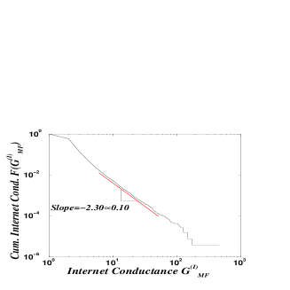
Figure 8: Cumulative distribution $F(G^{(I)}_{\rm MF})$ vs $G^{(I)}_{\rm MF}$ for the Internet. This slope is in good agreement with the scale-free structure that has been observed for the Internet (see text).

To test the validity of our model results in real networks, we measured the conductance $G^{(I)}_{\rm MF}$ on the most up to date map of the Autonomous Systems (AS) level of the Internet structure [31]. From Fig. 8 we find that the slope of the plot, which corresponds to $g_{G}-1$ from Eq. (9), is approximately 2.3, implying that $\lambda\approx 2.15\pm 0.05$, in agreement with the value of the degree distribution exponent for the Internet observed in [31]. Thus, transport properties can yield information on the topology of the network.

5 Multiple Sources

In many cases it is desirable to explore the more general situation, where the transport takes place between groups of nodes, not necessarily between a single source and a single sink. This might be a frequent scenario in systems such as the Internet, where data should be sent between a group of computers to another group, or in transportation network, where we can consider the quality of transport between e.g. countries, where the network of direct connections (flights, roads, etc.) between cities is already established.

The generalization of the above defined models is straightforward. For the electrical transport case, once we choose our $n$ sources and $n$ sinks, we simply wire the $n$ sources together to the positive potential $V=1$, and the $n$ sinks to $V=0$. For the max flow case, we connect the $n$ sources to a super-source with infinite capacity links, the same for the sinks. We then consider the max flow between the super-source and the super-sink.

For simplicity of notation, in this section we denote the electrical conductance with $G$ and the max-flow with simply $f$ (instead of $G_{MF}$).

The interesting quantity to consider in this case is the average conductance, or flow, per source, i.e. $\overline{G}/n$ or $\overline{f}/n$ (the averaging notation will be omitted when it is clear from the context), since this takes into account the obvious increase in transport due to the multiple sources. Considering the transport per source gives thus a proper indication of the network utilization.

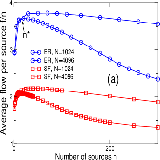
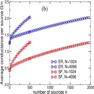
Figure 9: (a) The average flow per source, $f/n$ vs. the number of sources $n$, for ER and SF networks, and two values of network size $N$. For all curves there is an optimal $n^{*}$, for which the flow per source is maximized. Obviously, $n^{*}$ grows with $N$ such that the larger the network is, more users can use it in an optimal way. Above $n^{*}$, the flow per source decreases. (b) The average conductance per source, $G/n$ vs. the number of source $n$ again for ER, SF networks, and different network sizes. Here there is no optimal point– The more users in the network the more useful it is for transport. See the text for the qualitative explanation of this behavior.

In Fig. 9 we analyze the dependence of the transport on $n$. Consider first the case of max flow, in 9(a). It is seen, that the flow first increases with $n$, and then decreases, for both network models and network sizes. This observation is consistent with the transport backbone picture described above, if we generalize the definition of the transport backbone to include now all nodes in the network that are nor sources neither sinks. For small $n$ (or more precisely, $n\ll N$), the transport backbone remains as large, and hence as a good conductor, as it is in the case of a single source ($n=1$). Therefore, we expect again the flow to depend only on the degrees of the sources and the sinks. With one source and sink, the flow is confined by the smaller degree of the source and the sink. With multiple sources and sinks, the flow will be the minimum of
[sum of the degrees of the sources, sum of degrees of the sinks] . The more sources we have (larger $n$), the more chances for the sum of the degrees to be larger (since for a sum of many degrees to be smaller, we need all the degrees to be small, which is less probable). Thus for small $n$, $\overline{f}/n$ increases. An exact theory for this region is developed below. As $n$ grows larger, not only that the transport backbone becomes smaller, but the number of paths that need to go through it grows too. Therefore, many paths that were parallel before now require the simultaneous usage of the same link, and the backbone is no longer a perfect conductor. In other words, the interaction between the outgoing paths causes the decrease in the backbone transport capability.

From these two contradicting trends emerges the appearance of an optimal $n$, $n^{*}$. which is the $n$ for which the flow per source is maximized. This has an important consequences for networks design, since it tells us that a network has an optimal “number of users” for which the utilization of the network is maximized. Increasing or decreasing the number of nodes in each group, will force each node, on average, to use less of the network resources.

In Fig. 9(b), we plot the same for the electrical conductance case. But, in contrast to the flow case, here the conductance per source only increases with respect to the number of sources $n$. The reason is, that for large $n$, the number of parallel paths decrease, but their lengths decrease (since for so many sources and sinks, there is more probability for a direct or almost direct connection between some source and some sink), and therefore the conductance of each path significantly increase, such that the total flow increases too. All this did not affect the flow, since there, as mentioned in Section 4, the total flow do not depend on the distance between the source and the sink.

This fact, that electrical conductance improves with more sources, while flow only degrades, actually points out a fundamental difference between the two types of transport phenomena. This actually is a consequence of the arguments given in Section 4 as for the distance dependence, and completes the picture considering the comparison between the models.

For the max-flow model, a closed form formulas for $\overline{f}(n)$ and the probability distribution of the flow $\Phi_{\rm MF}(f)$ (for a given n) can be derived analytically in the region where $n\ll N$, where we can assume there is no interaction at all between the paths of the $n$ pairs, such that the flow is just the minimum of
[sum of the degrees of the source, sum of the degrees of the sinks] . A comparison between the theoretical formula and the simulation results will enable us to directly test this hypothesis; moreover it will mark the region ($n$ values) where “no interaction” between flow paths exist.

Next, we present the analytic derivation for small n. Denote by $k_{n}$ the sum of degrees of $n$ nodes. The total flow between $n$ sources and $n$ sinks is then given by $f=\min[k_{n}(\mbox{sources}),k_{n}(\mbox{sinks})]$. To calculate the distribution of flows (from which the average flow is found easily) one has first to calculate the distribution of the sum of $n$ iidrv’s $k_{1}$: $P_{k_{1}}(k)\sim k^{-\lambda},[k_{\rm min}\leq k\leq k_{\rm max}]$, for SF graphs, or $P_{k_{1}}(k)=\frac{\left(\overline{k}\right)^{k}e^{-\overline{k}}}{k!}$ for ER graphs. For $n\gg 1$, this is easy with the central limit theorem. However, for very large $n$, the effect of the interactions will begin to appear. Therefore, one should calculate the distribution of the sum directly, using convolution. If we consider the SF degree distributions to be discrete, The pdf of a sum of degrees of 2 nodes is then given by -

$$P_{k_{2}}(k)=\sum_{j=k_{min}}^{k-k_{min}}P_{k_{1}}(j)\cdot P_{k_{1}}(k-j)~{}~{}~{};~{}~{}~{}2k_{min}\leq k\leq 2k_{max},$$ (11)

which can be computed exactly in a computer, for a given $N,k_{min},\lambda$. The calculation can be easily extended to $n$ equals other pairs of 2. For ER networks, it is known that the sum of $n$ Poisson variables with parameter $\lambda$ is also a Poisson variable with parameter $n\lambda$. The probability distribution of the flow itself is readily calculated as the pdf of the minimum of the $k_{n}$’s, analogous to Eq. (8)–

$$\Phi_{\rm MF,n}(f)=2\cdot P_{k_{n}}(f)\cdot\left[\sum_{j=f}^{\infty}P_{k_{n}}(j)\right]-\left[P_{k_{n}}(f)\right]^{2}.$$ (12)

This can also be computed exactly in a computer, together with the average flow ($\overline{f}(n)=\sum_{f=1}^{\infty}f\cdot\Phi_{\rm MF,n}(f)$). However, for ER networks the sum can be solved:

$$\Phi_{\rm MF,n}(f)=2\frac{(n\lambda)^{f}e^{-n\lambda}}{f!}\left(1-\frac{\Gamma(f,n\lambda)}{\Gamma(f)}-\frac{1}{2}\frac{(n\lambda)^{f}e^{-n\lambda}}{f!}\right),$$ (13)

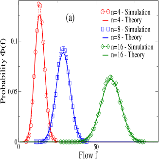
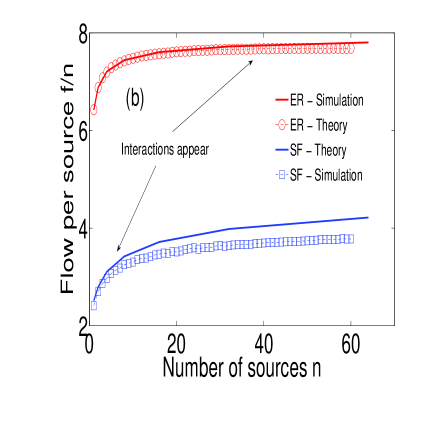
Figure 10: (a) For an ER network, with average degree $\overline{k}=4$, $N=8192$, we plot the probability distribution of the flows $\Phi_{\rm MF,n}$, for given $n=4,8,16$, as well as the theoretical prediction from Eq. (13). (b) For ER network with $\overline{k}=8$, $N=4096$, and SF network with $\lambda=2.4,k_{\rm min}=2$, $N=8192$, we plot the average flow per source, $\overline{f}$ vs. $n$, and compare it with the theoretical prediction under the assumptions of no interactions between the parallel paths. The number of sources where this assumption no longer holds is marked.

where $\Gamma(a)$ is the Gamma Function and $\Gamma(a,x)$ is the Incomplete Gamma Function. In Fig. 10, the “no-interactions” theory is compared to the simulation results, for small $n$. In panel (a), the pdf of the flows is shown for an ER network. The agreement between the theory and simulation is evident. In panel (b), we show the average flow per source, $\overline{f}/n$, as computed using Eq. (12), together with the simulation results, for ER and SF networks. The range of applicability of the no-interactions assumptions is clearly seen.

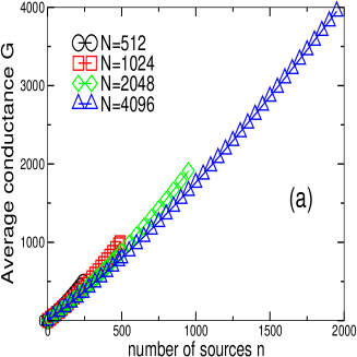
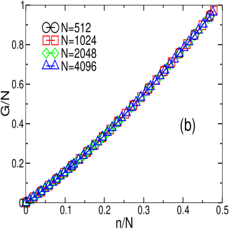
Figure 11: (a) The average conductance $\overline{G}$ is plotted vs. the number of sources $n$ for ER networks with average degree $\overline{k}$=4, and various values of network sizes $N$. (b) The same data, plotted now as $G/N$ with respect to $n/N$. With this scaling all the curves collapse, implying the scaling law $\overline{G}\sim Ng(n/N)$.

Scaling law for the conductance with multiple sources, is seen when properly scaling the conductance and the number of sources. Plotting $\overline{G}/N$ vs. $n/N$, (Fig. 11), all curves with different values of $N$ collapse. Thus we conclude the scaling form:

$$\overline{G}\sim Ng(n/N),$$ (14)

where $g(x)$ is a function of a single variable only. The same scaling appears for the flow as well (data not shown).

6 Summary

In summary, we find that the conductance of scale-free networks is highly heterogeneous, and depends strongly on the degree of the two nodes $A$ and $B$. We also find a power-law tail for $\Phi_{SF}(G)$ and relate the tail exponent $g_{G}$ to the exponent $\lambda$ of the degree distribution $P(k)$. This power law behavior makes scale-free networks better for transport. Our work is consistent with a simple physical picture of how transport takes place in scale-free and Erdős-Rényi networks, which presents the ’transport backbone’ as an explanation to the fact that the transport virtually depends only on the smallest degree of the two nodes. This scenario appears to be valid also for the frictionless transport model, as clearly indicated by the similarity in the results. We analyze this model and compare its properties to the electrical conductance case. We also compare our model results on a real network of the AS Internet and obtain good agreement. We then extend the study to transport with multiple sources, where the transport takes place between two groups of nodes. We find that this mode arises a fundamental difference between the behavior of the electrical and frictionless transport models. We also find an optimal number of sources in which the transport is most efficient, and explain its origin.

Finally, we point out that our study can be further extended. We could find a closed analytical formula, Eqs. (12), (13) for the distribution of flows in ER networks only. It would be useful to find an analytical formula also for SF networks, and in addition, to find a analytical form for the average flow (and conductance), per source. In other words, we need to find the scaling function $g(x)$ in Eq. (14). Also, it is of interest to investigate the dependence of the optimal number of sources, $n^{*}$, in the network size and connectivity. Finally, other, maybe more realistic, models for transport in a network with multiple sources should be considered.

7 Acknowledgments

We thank the Office of Naval Research, the Israel Science Foundation, the European NEST project DYSONET, and the Israel Internet Association for financial support, and L. Braunstein, R. Cohen, E. Perlsman, G. Paul, S. Sreenivasan, T. Tanizawa, and S. Buldyrev for discussions.

Figure 1: (a) Schematic of an Erdős-Rényi network of $N=12$ and $p=1/6$. Note that in this example ten nodes have $k=2$ connections, and two nodes have $k=1$ connections. This illustrates the fact that for Erdős-Rényi networks, the range of values of degree is very narrow, typically close to $\overline{k}$. (b) Schematic of a scale-free network of $N=12$, $k_{\rm min}=2$ and $\lambda\approx 2$. We note the presence of a hub with $k_{\rm max}=8$ which is connected to many of the other nodes of the network.

Figure 2: Comparison for networks with $N=8000$ nodes between the cumulative distribution functions of conductance for the Erdős-Rényi and the scale-free cases (with $\lambda=2.5$ and 3.3). Each curve represents the cumulative distribution $F(G)$ vs. $G$. The simulations have at least $10^{6}$ realizations.

Figure 3: (a) The pdf $\Phi_{\rm SF}(G|k_{A},k_{B})$ vs. $G$ for $N=8000$, $\lambda=2.5$ and $k_{A}=750$ ($k_{A}$ is close to the typical maximum degree $k_{\rm max}=800$ for $N=8000$). (b) Most probable values $G^{*}$, estimated from the maximum of the distributions in (a), as a function of the degree $k_{B}$. The data support a power law behavior $G^{*}\sim k_{B}^{\alpha}$ with $\alpha=0.96\pm 0.05$.

Figure 4: Scaled most probable conductance $G^{*}/k_{B}$ vs. scaled degree $x\equiv k_{A}/k_{B}$ for system size $N=8000$ and $\lambda=2.5$, for several values of $k_{A}$ and $k_{B}$: $\Box$ ($k_{A}=8$, $8\leq k_{B}\leq 750$), $\diamondsuit$ ($k_{A}=16$, $16\leq k_{B}\leq 750$), $\bigtriangleup$ ($k_{A}=750$, $4\leq k_{B}\leq 128$), $\bigcirc$ ($k_{B}=4$, $4\leq k_{A}\leq 750$), $\bigtriangledown$ ($k_{B}=256$, $256\leq k_{A}\leq 750$), and $\triangleright$ ($k_{B}=500$, $4\leq k_{A}\leq 128$). The curve crossing the symbols is the predicted function $G^{*}/k_{B}=f(x)=cx/(1+x)$ obtained from Eq. (7). We also show $G^{*}/k_{B}$ vs. scaled degree $x\equiv k_{A}/k_{B}$ for Erdős-Rényi networks with $\overline{k}=2.92$, $4\leq k_{A}\leq 11$ and $k_{B}=4$ (symbol $\bullet$). The curve crossing the symbols represents the theoretical result according to Eq. (7), and an extension of this line to represent the limiting value of $G^{*}/k_{B}$ (dotted-dashed line). The probability of observing $k_{A}>11$ is extremely small in Erdős-Rényi networks, and thus we are unable to obtain significant statistics. The scaling function $f(x)$, as seen here, exhibits a crossover from a linear behavior to the constant $c$ ($c=0.87\pm 0.02$ for scale-free networks, horizontal dashed line, and $c=0.55\pm 0.01$ for Erdős-Rényi, dotted line). The inset shows a schematic of the “transport backbone” picture, where the circles labeled $A$ and $B$ denote nodes $A$ and $B$ and their associated links which do not belong to the “transport backbone”.

Figure 5: (a) Simulation results for the cumulative distribution $F_{\rm SF}(G)$ for $\lambda$ between 2.5 and 3.5, consistent with the power law $F_{\rm SF}\sim G^{-(g_{G}-1)}$ (cf. Eq. (9)), showing the progressive change of the slope $g_{G}-1$. (b) The exponent $g_{G}-1$ from simulations (circles) with $2.5<\lambda<4.5$; shown also is a least square fit $g_{G}-1=(1.97\pm 0.04)\lambda-(2.01\pm 0.13)$, consistent with the predicted expression $g_{G}-1=2\lambda-2$ [cf. Eq. (9)].

Figure 6: (a) Cumulative distribution of link-independent paths (conductance) $F_{\rm MF}(G_{\rm MF})$ vs. $G_{\rm MF}$ compared with the electrical conductance distributions taken from Fig. 2. We see that the scaling is indeed the same for both models, but the proportionality constant of $F_{\rm MF}(G_{\rm MF})$ vs. $G_{\rm MF}$ is larger for the frictionless problem. (b) Scaled number of independent paths $G_{\rm MF}/k_{B}$ as a function of the scaled degree $k_{A}/k_{B}$ for scale-free networks of $N=8000$, $\lambda=2.5$ and $k_{\rm min}=2$. The behavior is sharp, and shows how $G_{\rm MF}$ is a function of only the minimum $k$.

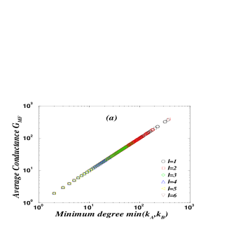
Figure 7: (a) Average conductance $\overline{G}_{\rm MF}$ vs. minimum degree $\min(k_{A},k_{B})$ of the source and sink $A$ and $B$ for different values of the shortest distance $\ell_{AB}$. The relation is independent of $\ell_{AB}$ indicating the independence of $\overline{G}_{\rm MF}$ on the distance. The network has $N=8000$, $\lambda=2.5$, $k_{\rm min}=2$. (b) Average conductance $\overline{G}$ vs. minimum degree $\min(k_{A},k_{B})$ of the source and sink $A$ and $B$ for different values of distance $\ell_{AB}$. The independence of $\overline{G}$ with respect to $\ell_{AB}$ breaks down and, as $\ell_{AB}$ increases, $\overline{G}$ decreases. Once again, $N=8000$ and $\lambda=2.5$, but the average has been performed for various $k_{B}<k_{A}$ and $k_{A}=750$.

References

- [1] S. Havlin and D. ben-Avraham, Adv. Phys. 36 (1987) 695-798.
- [2] D. ben-Avraham and S. Havlin Diffusion and reactions in fractals and disordered systems (Cambridge, New York, 2000).
- [3] A. Bunde and S. Havlin, eds. Fractals and Disordered Systems (Springer, New York, 1996).
- [4] R. Albert and A.-L. Barabási. Rev. Mod. Phys. 74 (2002) 47-97 ; R. Pastor-Satorras and A. Vespignani, Structure and Evolution of the Internet: A Statistical Physics Approach (Cambridge University Press, Cambridge, 2004); S. N. Dorogovsetv and J. F. F. Mendes, Evolution of Networks: From Biological Nets to the Internet and WWW (Oxford University Press, Oxford, 2003).
- [5] G. Bonanno, G. Caldarelli, F. Lillo, and R. N. Mantegna, Phys. Rev. E 68, 046130 (2003).
- [6] J.-P. Onnela, A. Chakraborti, K. Kaski, J. Kertész, and A. Kanto, Phys. Rev. E 68, 056110 (2003).
- [7] H. Inaoka, T. Ninomiya, K. Taniguchi, T. Shimizu, and H. Takayasu, Fractal Network derived from banking transaction – An analysis of network structures formed by financial institutions –, Bank of Japan Working Paper Series, 04-E-04 (2004). H. Inaoka, H. Takayasu, T. Shimizu, T. Ninomiya, K. Taniguchi, Physica A, 339, 62 (2004).
- [8] P. Erdős and A. Rényi, Publ. Math. (Debreccen), 6 (1959) 290-297.
- [9] B. Bollobás, Random Graphs (Academic Press, Orlando, 1985).
- [10] A.-L. Barabási and R. Albert, Science 286 (1999) 509-512.
- [11] P. L. Krapivsky, S. Redner, and F. Leyvraz, Phys. Rev. Lett. 85 (2000) 4629-4632.
- [12] H. A. Simon, Biometrika 42, 425 (1955).
- [13] R. Cohen, and S. Havlin, Phys. Rev. Lett. 89, 218701 (2002).
- [14] In principle, a node can have a degree up to , connecting to all other nodes of the network. The results presented here correspond to networks with upper cutoff imposed. We also studied networks for which is not imposed, and found no significant differences in the pdf .
- [15] E. López, S. V. Buldyrev, S. Havlin, and H. E. Stanley, Phys. Rev. Lett. 94 (2005) 248701.
- [16] S. Havlin, E. López, S. V. Buldyrev, H. E. Stanley: Anomalous Conductance and Diffusion in Complex Networks. In: Diffusion Fundamentals. (Ed. Jörg Kärger, Farida Grinberg, Paul Heitjans) Leipzig: Universitätsverlag, 2005, p. 38 - 48.
- [17] G. R. Grimmett and H. Kesten, J. Lond. Math. Soc. 30 (1984) 171-192; math/0107068.
- [18] D.-S. Lee and H. Rieger, Europhys. Lett. 73 (2006) 471-477.
- [19] Z. Toroczkai and K. Bassler, Nature 428 (2004) 716.
- [20] J. D. Noh and H. Rieger, Phys. Rev. Lett. 92 (2004) 118701.
- [21] V. Sood, S. Redner, and D. ben-Avraham, J. Phys. A, 38 (2005) 109-123.
- [22] L. K. Gallos, Phys. Rev. E 70 (2004) 046116.
- [23] The dynamical properties we study are related to transport on networks and differ from those which treat the network topology itself as evolving in time [10, 11].
- [24] The study of community structure in social networks has led some authors (M. E. J. Newman and M. Girvan, Phys. Rev. E 69 (2004) 026113, and F. Wu and B. A. Huberman, Eur. Phys. J. B 38 (2004) 331-338) to develop methods in which networks are considered as electrical networks in order to identify communities. In these studies, however, transport properties have not been addressed.
- [25] M. Molloy and B. Reed, Random Struct. Algorithms 6 (1995) 161-179.
- [26] G. Kirchhoff, Ann. Phys. Chem. 72 (1847) 497 ; N. Balabanian, Electric Circuits (McGraw-Hill, New York, 1994).
- [27] S. Kirkpatrick, ”Percolation Thresholds in Granular Films – Non-Universality and Critical Current”, Proceedings of Inhomogeneous Superconductors Conference, Berkeley Springs, W. Va, edited by S.A. Wolf and D. U. Gubser, A.I.P. Conf. Procs. 58 (1979) 79.
- [28] B. V. Cherkassky, Algorithmica 19 (1997) 390.
- [29] Z. Wu, L. A. Braunstein, S. Havlin, and H. E. Stanley Phys. Rev. Lett. 96 (2006) 148702.
- [30] S. Carmi, S. Havlin, S. Kirkpatrick, Y. Shavitt and E. Shir, ”MEDUSA - New Model of Internet Topology Using k-shell Decomposition”, arXiv, cond-mat/0601240.
- [31] Y. Shavitt and E. Shir, ACM SIGCOMM Computer Communication Review, 35(5) (2005) 71.