Self-consistent calculation of the electron distribution near a Quantum-Point Contact in the integer Quantum Hall Effect

Abstract

In this work we implement the self-consistent Thomas-Fermi-Poisson approach to a homogeneous two dimensional electron system (2DES). We compute the electrostatic potential produced inside a semiconductor structure by a quantum-point-contact (QPC) placed at the surface of the semiconductor and biased with appropriate voltages. The model is based on a semi-analytical solution of the Laplace equation. Starting from the calculated confining potential, the self-consistent (screened) potential and the electron densities are calculated for finite temperature and magnetic field. We observe that there are mainly three characteristic rearrangements of the incompressible ”edge” states, which will determine the current distribution near a QPC.

I Introduction

A quantum point contact (QPC) is constructed by geometric or electrostatic confinement of a two dimensional electron system (2DES). The conductance through them is quantized van Wees et al. (1988); Wharam et al. (1988) and they play a crucial role in the field of mesoscopic quantum transport. Their properties have been investigated in a wide variety of experiments, which include the observation of the 0.7 anomaly Thomas et al. (1996a, b), quantum dots coupled to QPCs Khrapai et al. (submitted to Phys. Rev. Lett), Quantum-Hall effect (QHE) based Mach-Zender Ji et al. (2003); Neder et al. (2006) and Aharonov-Bohm interferometers. This has lead to extensive investigations of the electrostatic and transport properties of QPCs, both with and without a quantizing magnetic field. Many different techniques have been used to find the electronic density distribution near a QPC, ranging from numerical Poisson–Schrödinger solutions Fiori et al. (2002) to spin-density-functional theory Hirose et al. (2003) and phenomenological approaches Reilly et al. (submitted to Physica E). It has been possible to treat realistic samples mostly only within simplified electrostatic calculations, neglecting screening effects. On the other hand, when including interactions the calculations become more complicated, thus one usually sacrifices handling realistic geometries.

Recent experiments have succeeded in developing and analyzing a QHE based electronic Mach-Zender interferometer (MZI) Ji et al. (2003), making use of the integer QHE edge states Neder et al. (2006) as single-channel chiral quantum wires. A key element of these experiments are the QPCs, which play the role of the beam splitters of the optical setup. The electrostatic potential and electronic density distributions in and near the QPCs play an important role in understanding the rearrangement of the edge states involved. Moreover, the electron-electron interaction has been proposed Neder et al. (2006) as one of the origins of dephasing in such an electronic MZI, such that a self-consistent calculation of the electrostatic potential may also be viewed as a first step towards a quantitative understanding of this issue. So far, the theoretical description of dephasing in the electronic MZI via classical Seelig and Büttiker (2001); Marquardt and Bruder (2004a, b); Förster et al. (2005) or quantum noise fields Marquardt (2005, 2006) and other approaches Pilgram et al. (2005) has focused on features supposed to be independent of its specific realization (see Ref. [Marquardt, to be published in: ,,Advances in Solid State Physics”, Vol. 46, ed. R. Haug, Springer 2006] for a recent review). However, a more detailed analysis of the QHE related physics, taking account of interaction effects, will certainly be needed for a direct comparison with experimental data. In this paper, we will provide a detailed numerical analysis of the electrostatics of QPCs in the integer QHE, assuming geometries adapted to those used in the MZI experiment. Our work will produce the electron density and electrostatic potential, based on the self-consistent Thomas-Fermi-Poisson approximation, to which we refer as TFA in the following.

We would like to point out the following observation regarding the Mach-Zehnder experiment, where a yet-unexplained beating pattern observed in the visibility (interference contrast) as a function of bias voltage was surprisingly found to have a period independent of the length of the interferometer arms. Such a result would seem less surprising if all the relevant interaction physics leading to the beating pattern were actually taking place in the vicinity of the QPC. This provides strong encouragement for future more detailed work on the coherent transport properties of these QPCs.

Although it has been more than two decades since the discovery of the quantized Hall effect v. Klitzing et al. (1980), the microscopic picture of current distribution in the sample and the interplay of the current distribution with the Hall plateaus is still under debate. In recent experiments, the Hall potential distribution and the local electronic compressibility have been investigated in a Hall bar geometry by a low-temperature scanning force microscope Ahlswede et al. (2002) and by a single-electron-transistor Ilani et al. (2000), respectively. This has motivated theoretical Güven and Gerhardts (2003) work, where a self-consistent TFA calculation has been used to obtain electrostatic quantities.

Self-consistent screening calculations show that the 2DES contains two different kinds of regions, namely the quasi-metallic compressible and quasi-insulating incompressible regions Chklovskii et al. (1992); Siddiki and Gerhardts (2003). The electron distribution within the Hall bar depends on the ”pinning” of the Fermi level to highly degenerate Landau levels. Wherever the Fermi level lies within a Landau level with its high density of states (DOS), the system is known to be compressible (leading to screening and correspondingly to a flat potential profile), otherwise it is incompressible, with a constant electron density and, in general, a spatially varying potential due to the absence of screening. Moreover, based on these results for the potential and density distributions, one may employ a local version of Ohm’s law (together with Maxwell’s equations and an appropriate model for the conductivity tensor) to calculate the current distribution, imposing a given overall external current for the in-plane geometry . These results are mostly consistent with experiments except that within the self-consistent TFA one obtains an incompressible strip (IS) for a large interval of magnetic field values which leads to coexistence of several IS’s with different local filling factors. Recently, this theory has been improved in two aspects Siddiki and Gerhardts (2004a, b): (i) the finite extent of the wave functions was taken into account in obtaining electrostatic quantities (rather than using delta functions), (ii) the findings of the full Hartree calculations were simulated by a simple averaging of the local conductivities over the Fermi wave length , thereby relaxing the strict locality of Ohm’s law for realistic sample sizes. A very important outcome of this model is that there can exist only one incompressible edge state at one side of the sample for a given magnetic field value. Indeed this is differing drastically from the Chklovskii-Shklovskii-Glazman (CSG) Chklovskii et al. (1992) and the Landauer-Büttiker Büttiker (1988) picture, where more than one edge state can exist and is necessary to ”explain” the QHE. In the CSG scheme a non-self-consistent TFA (which is called the ”electrostatic approximation”) was used. However, it is clear that if the widths of the IS’s (where the potential variation is observed) become comparable with the magnetic length, the TFA is not valid, thus the results obtained within this model are not reliable any more. In principle, similar results to Ref. [Siddiki and Gerhardts, 2004a] were reported by T. Suzuki and T. Ando Suzuki and Ando (1993), quite some time ago and recently by S. Ihnatsenka and I. V. Zozoulenko Ihnatsenka and Zozoulenko (2006) in the context of spin-density-functional theory. With the improvements on the self-consistent TFA mentioned above, together with taking into account the disorder potential Siddiki and Gerhardts (submitted to Int. J. Mod. Phys. B) and using the self-consistent Born approximation Ando et al. (1982) to calculate the local conductivity tensor, one obtains well developed Hall plateaus, with the longitudinal resistivity vanishing to a very high accuracy, and one is also able to represent correctly the inter-plateau transition regions. Wherever one observes an IS, the longitudinal conductivity becomes zero, and as a consequence also the corresponding local resistance (and the total resistance) vanishes. Thus, according to Ohm’s law, the current flows through the incompressible region. In addition, the Hall conductance becomes equal to the local value of the quantized conductance. Finally all the three experimentally observed Ahlswede et al. (2001) qualitatively different regimes of how the Hall potential drops across the sample have been reproduced theoretically without artifacts of the TFA Güven and Gerhardts (2003). The model described above has also been successfully applied to an electron-electron bilayer system Siddiki (submitted to Phys. Rev. B) and provided a qualitative explanation Siddiki et al. (2006) of the magneto-resistance hysteresis that has been reported recently Tutuc et al. (2003); Pan et al. (2004). For all of these reasons, we feel confident in applying this theory to our analysis of the MZI setup.

Motivated by the experimental and theoretical findings ascertaining the importance of the interaction effects in the integer Quantum Hall regime, in this work we will show that the mutual Coulomb interaction between the electrons leads to interesting non-linear phenomena in the potential and electron distribution in close proximity of the QPCs. Based on the self-consistent Thomas-Fermi-Poisson approximation (TFA), we will consider realistic QPC geometries and examine the distribution of the incompressible regions depending on the field strength and sample parameters.

The rest of this paper is organized as follows: In Sec. II the electrostatic potential produced by an arbitrary surface gate will be discussed, by solving the Laplace equation without screening effects. In Sec. III we review the TFA in a 2DES. In Sec. IV we will first present the well known general results of the TFA for a homogeneous 2DES at zero magnetic field $B$ and zero temperature, and we will investigate the electron density and electrostatic potential profiles of a (i) simple square gate geometry and (ii) a generic QPC, before (iii) systematically investigating the positions of the incompressible strips depending on magnetic field and geometric parameters. We conclude with a discussion in Sec. V

II Electrostatics of the gates

As mentioned in the introduction, there is a tradeoff between simulating realistic QPC geometries and including the interaction effects within a reasonable approximation. In this paper, we present an intermediate approach, which considers realistic QPC structures but interactions of the electrons are handled within a Thomas-Fermi approximation (TFA), which is valid for relatively ”large” QPCs ($\gtrsim 100$ nm). One can obtain, in a semi-analytical fashion, the electrostatic potential generated by an arbitrary metallic gate at the surface by solving the Laplace equation for the given boundary conditions. Afterwards, it is possible to obtain the electron and potential distribution in the 2DES, within the TFA, both for vanishing and finite magnetic fields ($B$), and at low temperatures at $B>0$.

Here we briefly summarize the semi-analytical model developed by J.Davies and co-workersDavies et al. (1995). The aim of this section is to calculate the electrostatic potential on a plane at some position $z$ below the surface of the semiconductor, which is partially covered by a patterned gate. The surface occupies the $z=0$ plane and z is measured into the material. The un-patterned surface is taken to be pinned so we can set the potential $V_{up}({\bf{r}},0)=0$ there, with $V_{gate}({\bf{r}},0)=V_{g}$ on the gate. We use lower-case letters like ${\bf{r}}=(x,y)$ to denote two-dimensional vectors with the corresponding upper-case letters for three dimensional vectors like ${\bf R}=(x,y,z)=({\bf r},z)$. Thus the problem is to find a solution, $V_{ext}({\bf{R}})$, to the Laplace equation $\nabla^{2}V_{ext}=0$, given the value on the plane $z=0$, and subject to the further boundary condition $\partial V_{ext}/\partial z\rightarrow 0$ as $z\rightarrow\infty$.

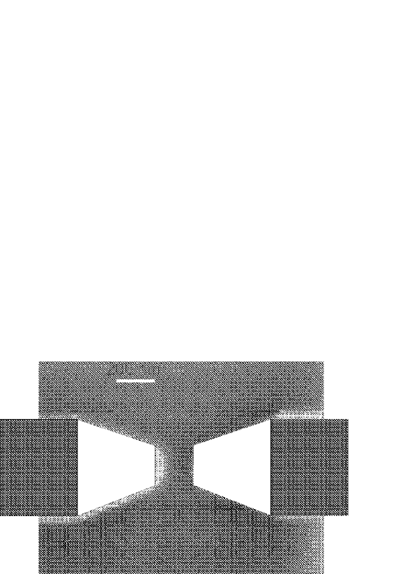
Figure 1: The image of the QPC (gray scale). The polygons are used to define the gates on the two-dimensional mesh. The 2DES resides under the dark (grey) regions, with a bulk electron density of $1.7\times 10^{-11}cm^{-2}$ (see Ref. [Ji et al., 2003], due to memory limitations the quality of the figure is reduced. The white line scales $200$nm).

One route is to start by making a two-dimensional Fourier transform from $V_{ext}({\bf{r}},0)$ to $\tilde{V_{ext}}({\bf{q}},0)$. The dependence on z is a decaying exponential to satisfy Laplace s equation and the boundary condition at $z=\infty$: $\tilde{V}_{ext}({\bf{q}},z)=\tilde{V}_{ext}({\bf{q}},0)\exp(-|qz|)$. This multiplication of the Fourier transform is equivalent to a convolution in real space. Taking the two-dimensional inverse Fourier transform of $\exp(-|qz|)$ leads to the general result.

$$V_{\rm{ext}}({\bf{r}},z)=\frac{1}{\kappa}\int{\frac{|z|}{2\pi(z^{2}+|{\bf{r}}-{\bf{r^{\prime}}}|^{2})^{3/2}}}V_{gate}({\bf{r^{\prime}}},0)d{\bf{r^{\prime}}},$$ (1)

where $\kappa$ is the dielectric constant of the considered hetero-structure. Now one can evaluate the potential in the plane of the 2DES, $z=d$, for a given gate and potential distribution on the surface. The derivation of some important shapes like triangle, rectangle and polygons is provided in the work cited above, which has been successfully applied to quantum dot systemsHuettel et al. (to be submitted to Phys. Rev. B). For our geometry, we will use the result for the polygons.

III Electron-electron interaction: Thomas-Fermi-Poisson Approximation

The main assumption of this approximation is that the external (confining) potential varies smoothly on the length scale of the magnetic length, $l_{b}=\sqrt{\hbar/(m\omega_{c})}$, where $m$ is the effective mass of an electron in a GaAs/AlGaAs hetero-structure, and $\omega_{c}$ is the cyclotron frequency given by $\omega_{c}=eB/m$ for the magnetic field strength $B$. At the magnetic field strengths of our interest, where the average filling factor ($\bar{\nu}$) is around 2, i.e. $B>5T$, $l_{b}$ is on the order of 10 nanometers, hence the TFA is valid. We note that spin degeneracy will not be resolved in our calculations. This can be done if the cyclotron energy is much larger than the Zeeman energy (i.e. effectively we set $g=0$).

In the following, we briefly summarize the self-consistent numerical scheme adopted in this work. We will assume the 2DES to be located in the plane $z=85$nm with a (surface) number density $n_{\rm el}(x,y)$. We consider a rectangle of finite extent $a_{x}\times a_{y}$ in the $xy$-plane, with periodic boundary conditions. The (Hartree) contribution $V_{H}(x,y)$ to the potential energy of an electron caused by the total charge density of the 2DES can be written as Oh and Gerhardts (1997)

$$V_{H}(x,y)=\frac{2e^{2}}{\bar{\kappa}}\int_{0}^{a_{x}}\int_{0}^{a_{y}}\!dx^{\prime}\!dy^{\prime}K(x,x^{\prime},y,y^{\prime})\,n_{\rm el}(x^{\prime},y^{\prime}),$$ (2)

where $-e$ is the electron charge, $\bar{\kappa}$ an average background dielectric constant, Oh and Gerhardts (1997) and the kernel $K(x,x^{\prime},y,y^{\prime})$ describes the solution of Poisson’s equation with appropriate boundary conditions. This kernel can be found in a well known text book Morse and Feshbach (1953). The electron density in turn is calculated in the Thomas-Fermi approximation (TFA) Oh and Gerhardts (1997)

$$n_{\rm el}(x,y)=\int dE\,D(E)f\big{(}[E+V(x,y)-\mu^{\star}]/k_{B}T\big{)},$$ (3)

with $D(E)$ the relevant (single-particle) density of states (DOS), $f(s)=[1+e^{s}]^{-1}$ the Fermi function, and $\mu^{\star}$ the electrochemical potential. The total potential energy of an electron, $V(x,y)=V_{\rm ext}(x,y)+V_{H}(x,y)$, differs from $V_{H}(x,y)$ by the contribution due to external potentials, e.g. the confinement potential generated by the QPC (see figure 3), potentials due to the donors etc. The local (but nonlinear) TFA is much simpler than the corresponding quantum mechanical calculation and yields similar results if $V(x,y)$ varies slowly in spaceSiddiki and Gerhardts (2004a), i.e. on a length scale much larger than typical quantum lengths such as the extent of wave functions or the Fermi wavelength.

IV Numerical calculations

The equations (2) and (3) have to be solved self-consistently for a given temperature and magnetic field, until convergence is obtained. In our scheme we start with vanishing field and at zero temperature to obtain the electrostatic quantities and use these results as an initial value for the finite temperature and field calculations. For $B,T>0$ we start with a relatively high temperature and reduce $T$ stepwise in order to obtain a good numerical convergence.

IV.1 Zero magnetic field

In this section we review the theory of screening in a homogeneous 2DES.

Mesoscopic systems like quantum dots, Hall bars, or any edges of quasi-2D electron systems are defined by lateral confinement conditions, which lead to an inhomogeneous electron density. An exact treatment of the mutual interactions of the electrons in such systems is only possible for quantum dots with very few (less than ten) electrons.

The total potential seen by any electron is given by the sum of the external potential (describing the confinement) and the Hartree potential given by Eq. (2), where the electron density in turn is determined self-consistently by the effective single-particle potential $V_{ext}+V_{H}$.

Now consider a 2DES in the $xy$- plane (with vanishing thickness) and having the charge density

$$n_{el}^{3D}(\vec{r})=n_{el}^{2D}({\bf r})\delta(z)=\int\frac{d^{2}q}{(2\pi)^{2}}n^{q}e^{i{\bf qr}}\delta(z)$$ (4)

with ${\bf q}=2\pi(n_{x}/a,n_{y}/b)$, where $n^{q}$ is the $q$- component of the Fourier transformed electron density. We want to obtain the effects of an external perturbation $\delta V_{ext}({\bf r},z)$, whose Fourier components in the plane $z=0$ are $\delta V_{ext}^{q}(0)$. This potential induces a charge density $\delta n^{q}$, which in turn leads to an induced potential

$$\delta V_{ind}^{q}(z)=\frac{2\pi e^{2}}{\kappa q}e^{-q|z|}\delta n^{q},$$ (5)

that has the tendency to screen the applied external potential. Within the TFA, the induced density is related to the overall screened potential $V_{scr}$ by $\delta n^{q}=-D_{T}^{2D}\delta V_{scr}^{q}(0)$, where $D_{T}^{2D}$ is the thermodynamic DOS defined as $D_{T}=\int dED(E)\frac{df}{d\mu}$.

Employing $\delta V_{scr}=\delta V_{ext}+\delta V_{ind}$, this yields

$$\delta V_{scr}^{q}(0)=\frac{\delta V^{q}_{ext}(0)}{\varepsilon({\bf q})},$$ (6)

where

$$\varepsilon({\bf q})=1+\frac{q_{TF}}{q}$$ (7)

is the 2D dielectric function with the Thomas-Fermi momentum

$$q_{TF}=\frac{2\pi e^{2}}{\kappa}D_{T}^{2D}.$$ (8)

Then the self-consistent potential at distance $|z|$ from the 2DES is

$$\delta V_{scr}^{q}(z)=\delta V_{ext}^{q}(z)-\frac{q_{TF}}{q+q_{TF}}e^{-q|z|}\delta V_{ext}^{q}(0),$$ (9)

i.e., the screening effect of the 2DES decreases exponentially with $|z|$.

In the limit $B=0$, $T\rightarrow 0$ and with $E_{F}=\mu^{\star}(B=0,T=0)$, Eq. (3) reduces to

$$n_{\rm el}(x,y)=D_{0}\,\big{(}E_{F}-V(x,y)\big{)}\,\theta\big{(}E_{F}-V(x,y)\big{)},$$ (10)

where $D_{0}$ is the constant DOS for a 2DES given by $D_{0}=m/(\pi\hbar^{2})$. This is a linear relation between $V(x,y)$ and $n_{\rm el}(x,y)$ for all $V(x,y)<E_{F}$.

Now we apply these results to determine the screening of a given periodic charge distribution in the plane $z=0$, which creates an external potential $V_{ext}({\bf r},0)=\sum_{q}V^{q}e^{i{\bf qr}}$ in this plane. The self-consistent potential in a 2DES then is described by:

$$V_{scr}(\textbf{r},z)=\sum_{q}V_{scr}^{q}(z)e^{i{\bf qr}},\quad\quad V_{scr}^{q}(z)=V^{q}e^{-qz}\big{(}1+\frac{2}{qa_{\rm B}^{\star}}\big{)}^{-1}.$$ (11)

The dielectric function $\epsilon(q)$ can be expressed in terms of the effective Bohr radius $a_{\rm B}^{\star}=\bar{\kappa}\hbar^{2}/(me^{2})$ (for GaAs $a_{\rm B}^{\star}=9.8\,$nm), sinceStern (1967); Wulf et al. (1988) $2/a_{\rm B}^{\star}=2\pi e^{2}D_{0}/\bar{\kappa}$, with $q=2\pi/a$. We will assume that $\varepsilon(q)\gg 1$, so that the TFA is valid for $B\gtrsim 1\,$T, i.e. $l_{m}\lesssim 30\,$nm. We also note that the $q=0$ component is cancelled by the homogeneous donor distribution, assuring overall charge neutrality.

IV.2 Simple example: Square gate barrier

We start our discussion by a simple example that presents the features of non-linear screening in a 2DES. We assume a negatively charged metallic square gate depicted by the white area in the inset of 2a, located at the center of a cell that is periodically continued throughout the plane (with periods $a_{x}=a_{y}=600$nm). The square is of size $200$nm, and it is kept at the gate potential, $V_{gate}=-0.1$V. In Fig.2 we show the external and the screened potential for different separation distances of the 2DES and the gate, calculated along the dashed line shown in the inset, in the plane of the 2DES.

In the left panel, the external potential has been plotted, with the dashed line representing the barrier (gate potential) on the surface. We observe that the potential profile becomes smooth quickly due to the exponential decay of the amplitude of Fourier components at large $q$ with increasing $z$Siddiki (2005).

In contrast, the screened potential displays an interesting, strong feature close to the edges of the gate ($x\sim 200$ and $x\sim 400$), when the separation distance is relatively small ($z<60$nm). This is nothing but the manifestation of the $q$ dependent screening given in Eq.( 11): The large $q$ components of the potential remain (almost) unaffected by screening, whereas the low $q$ (long wavelength) components are well screened. As a result, we observe sharp peaks near the edge of the gate for small distances $z$, which turn into ”shoulders” at larger $z$. We should caution, however, that for $z<60$nm the validity of the TFA may become questionable, since the potential then changes rapidly on the scale of the Fermi wavelength.

This simple example already demonstrates the strongly non-linear behavior of the screening, which can be summarized as follows: (i) the strongly varying part (high $q$ components) of the external potential remains (almost) unscreened by the 2DES, but its amplitude decreases fast with increasing separation $z$, whereas (ii) the slowly varying part (small $q$ components) is well screened by the 2DES, but its amplitude decays much slower for large separation distances. Indeed this non-linearity ($q$-dependence of $\varepsilon$) leads to peculiar effects both on electrostatics and transport properties of the QPCs, depending on the geometry and the structure of the sample. In the next section we will look for such effects with regard to the QPCs.

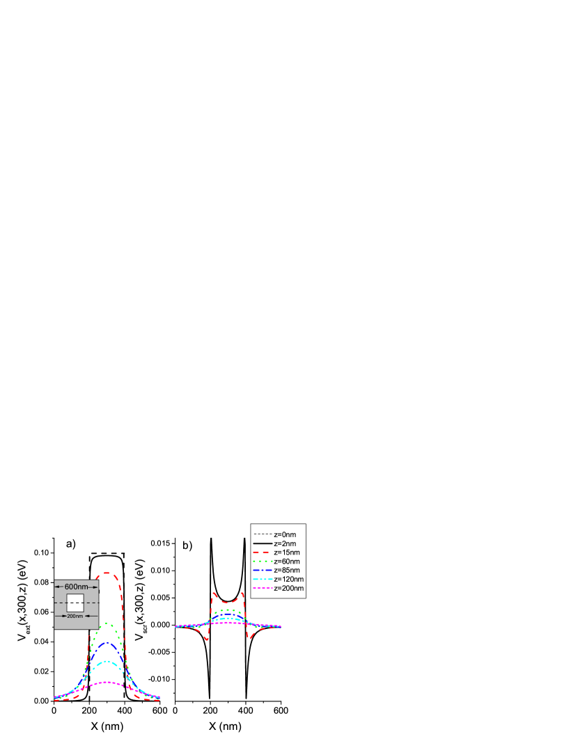
Figure 2: External potential (left panel) seen by a 2DES at different distances z and the corresponding screened potentials (right panel). The separating dielectric material is assumed to be GaAs with $\kappa=12.4$ and the calculations are done at $T=0$K.

IV.3 Simulation of the QPC

In this section we will first obtain the bare confinement potential created by the QPC for the geometry given in figure 1, and then go on to discuss the effects of screening. The potential generated by such gates can be calculated by the scheme proposed by Davies et al.Davies et al. (1995).

The model parameters are taken from the relevant experimental samplesNeder et al. (2006); Ned , where the applied gate voltage is $-0.3$V, the width at the tip is about $200$nm, and the tip separation $\Delta y\sim 300$nm. The 2DES is taken to be $85$nm below the surface.

We define the QPC using rectangles and polygons which are shown in figure 1 as red (dark) and white areas. In figure 3 we show the bare confining potential for the parameters given above. The electrons are filled up to the Fermi energy ($E_{F}\sim 7$meV, corresponding to a typical electron surface density $n_{el}\sim 1.7\times 10^{11}$ cm^-2). Using such parameters, the full screening calculation to be discussed below will reveal the electrons to be depleted beneath the QPC, say at all the dark (blue) regions in Fig.4.

In our numerical simulations, we have mapped the unit cell containing the QPC of physical dimensions $3.3\mu$m$\times 1.8\mu$m to a matrix of 200 by 200 mesh points in the absence of a magnetic field and $1.1\mu$m$\times 1.8\mu$m to a matrix of 48 by 96 mesh points in the presence, which allows us to perform numerical simulations within a reasonable computation time. With regard to numerical accuracy, we estimate that, for typical electron densities, the mean electron distance, i.e. the Fermi wavelength, is larger than 40nm. Hence, the number of mesh points considered here allows us to calculate the electron density with a good numerical accuracy. We also performed calculations for finer meshes and the results do not differ quantitatively (at the accuracy of line thicknesses), whereas the computational time grows like the square of the number of the mesh points. We should also note that due to computation time concerns we had to use a smaller unit cell in the presence of the magnetic field, which yields finite size effects close to the boundaries of the sample (e.g. see Fig 7b). The features observed are, in principle, negligible and they tend to disappear when the unit cell is taken to be larger and mapped on a larger matrix.

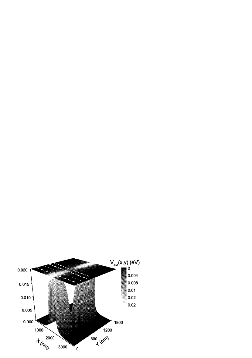
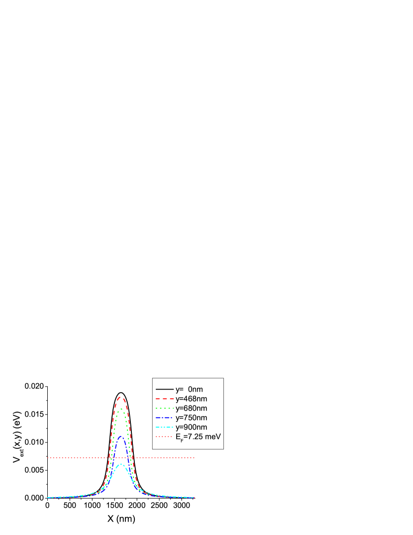
Figure 3: The bare confinement potential generated by the QPC, defined by the polygons shown in figure 1. The color scale indicates the strength of the confinement.

We now discuss the resulting bare and screened potential for a realistic QPC defined by surface gates, with a tip opening $\Delta y=$ $300$nm. Figure 3 represents the external potential created by the QPC gate structure at the surface, calculated in the plane of the 2DES located at $z=85$nm below the surface, with an applied potential $-0.3$V. In the upper panel we show a 3D plot and a planar projection, together with four guide lines, which indicate the location of the cross-sections through the that are displayed in the lower panel. The level of the Fermi energy of the system (to be assumed below) is indicated in the 3D plot as well. These results have been obtained numerically from Eq. (1). The barrier is formed by the regions of elevated potential.

At the first glance one observes that the potential landscape is smoothly varying. This is purely an effect of the relatively large distance to the gate, as screening effects have not yet been included. For the given Fermi energy (obtained from the electron density in the bulk) and the tip separation, $\Delta y\gtrsim 100$ nm, the number density of electrons inside the QPC opening fulfills the validity relation of the TFA, i.e. $n_{el}(\rm{center})a_{B}^{\star}\gg 1$. At the positions where the height of the barrier becomes larger than the Fermi energy (light line in the 3D plot and horizontal dashed line in the lower panel), the probability to find an electron is zero within the TFA.

We proceed in our discussion with a comparison of the screened potential shown in Fig. 4 to the bare confinement potential discussed up to now (Fig. 3). The self-consistent potential is obtained from the formalism described above for periodic boundary conditions at zero temperature and zero magnetic field. The electrons are filled up to the Fermi energy (shown by the gray thick line on the surface of the color plot and dashed line in the lower panel), such that no electrons can penetrate classically into the barrier above those lines. The first observation is that the potential profile becomes sharper for the screened case and strong variations are observed in the vicinity of the QPC. These shoulder-like local maxima near the QPC represent the same feature seen in the example of the square barrier discussed previously, and we have pointed out that they stem from $q$-dependent, non-linear screening. This will become more important when we consider a magnetic field, since the local ”pinning” of the Landau levels to the Fermi energy in these regions will produce compressible regions surrounded by incompressible regions.

An interesting feature occurs near the opening of the QPC, namely a local minimum which is a result of the non-linear screening. We point out that somewhat similar physics has been found (using spin-density-functional theoryHirose et al. (2003)) to lead to the formation of a local bound state inside a QPC, which has been related to the ”0.7” anomaly, linking it with Kondo physics. We believe this feature to be a very important result of the self-consistent screening calculation, and we note that it may affect strongly the transport properties of the QPC both in the presence or absence of a magnetic field. We will discuss the influence of this local minimum on the formation of the incompressible strips in section IV.4, where we calculate the density and potential profiles including a strong perpendicular magnetic field.

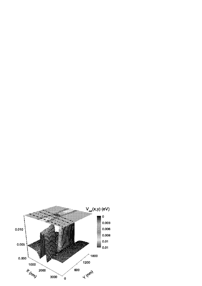
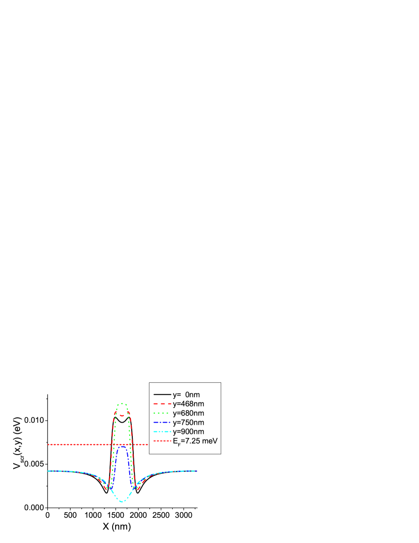
Figure 4: The screened potential (upper panel) seen by a 2DES at $85$nm below the surface and some characteristic cuts along the $x$- axis, together with an indication of the Fermi level $E_{F}$ (lower panel). The color scale represents the strength of the potential, and the cross-sections are indicated by the same line code as in Fig. 3.

It is known from the experiments that the interference pattern and the transmission properties strongly depend on the structure of the QPCs, such as the distance of the 2DES from the surface, the applied gate voltage, the sharpness and the geometry of the edges, as well as the width of the opening of the QPC. The effect of the first two parameters can be understood by following the simple arguments of linear screening as shown for the square gate model: if the distance from the QPC to the 2DES increases, the potential profile becomes more and more smooth. The screened potential changes linearly with the applied gate potential (see Eq.(11)). The geometric parameters have to be adapted to the experiment in question. Note that the shape of the QPCs has already been discussed in the literature (see Ref. Fiori et al., 2002 and references contained therein). The effect of the size of the QPCs, however, has not been considered for large $\Delta y$ ($>100$nm), and we believe this to be an important parameter for the interferometer experiments.

We start our investigation by looking at the opening of the QPC with increasing tip separation of the metal gates used to define the QPC. In this section, we work at zero temperature and magnetic field, with a constant bulk electron density.

In figure 5 we depict the self-consistent potential at the center of the QPC ($y=550$nm), while changing the tip separation ($\Delta y$) between $100$ and $500$nm. We see that for the narrowest separation the potential profile looks rather smooth and a minimum is observed at the center. If we increase $\Delta y$($\leqslant 300$nm) we see that the screening becomes stronger, leading to more pronounced shoulders on the sides and a deeper minimum at the center. For even larger separations ($\Delta y>300$nm) a local maximum starts to develop at the center, since the electrostatic potential energy is no longer strong enough to repel the electrons from this region. Basically all the non-linear features observed result from the competition between the gate potential, which simply repels the electrons, and the mutual Coulomb interaction, i.e. the Hartree potential. It is obvious that for narrower tip separations only a few electrons will remain inside the QPC opening and therefore TFA type approximations will not be justified any longer.

Summarizing this section, we have determined the screened potential profile in a realistic QPC geometry, pointing out features resulting from non-linear screening. We have observed that a local extremum occurs at the center of the QPC, and have traced the dependence on the width $\Delta y$ between the QPC tips. These features, as mentioned before, become more interesting if a magnetic field is also taken into account, where they lead to stronger spatial inhomogeneities in the electron distribution. Our next step is thus to include a strong quantizing perpendicular magnetic field and examine the distribution of the incompressible strips where the imposed external current is confinedAhlswede et al. (2002); Siddiki and Gerhardts (2004a).

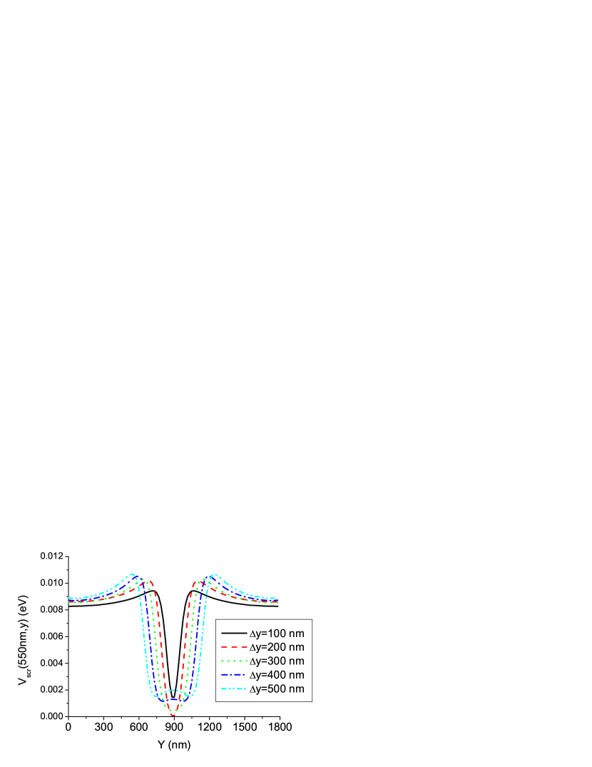
Figure 5: The screened potential at $x=550$nm for five different tip distances. Note that the $x$ interval used for the calculation smaller than in the previous figure, since we concentrate on the bulk structures rather than the edge ones.

IV.4 Finite temperature and Magnetic field

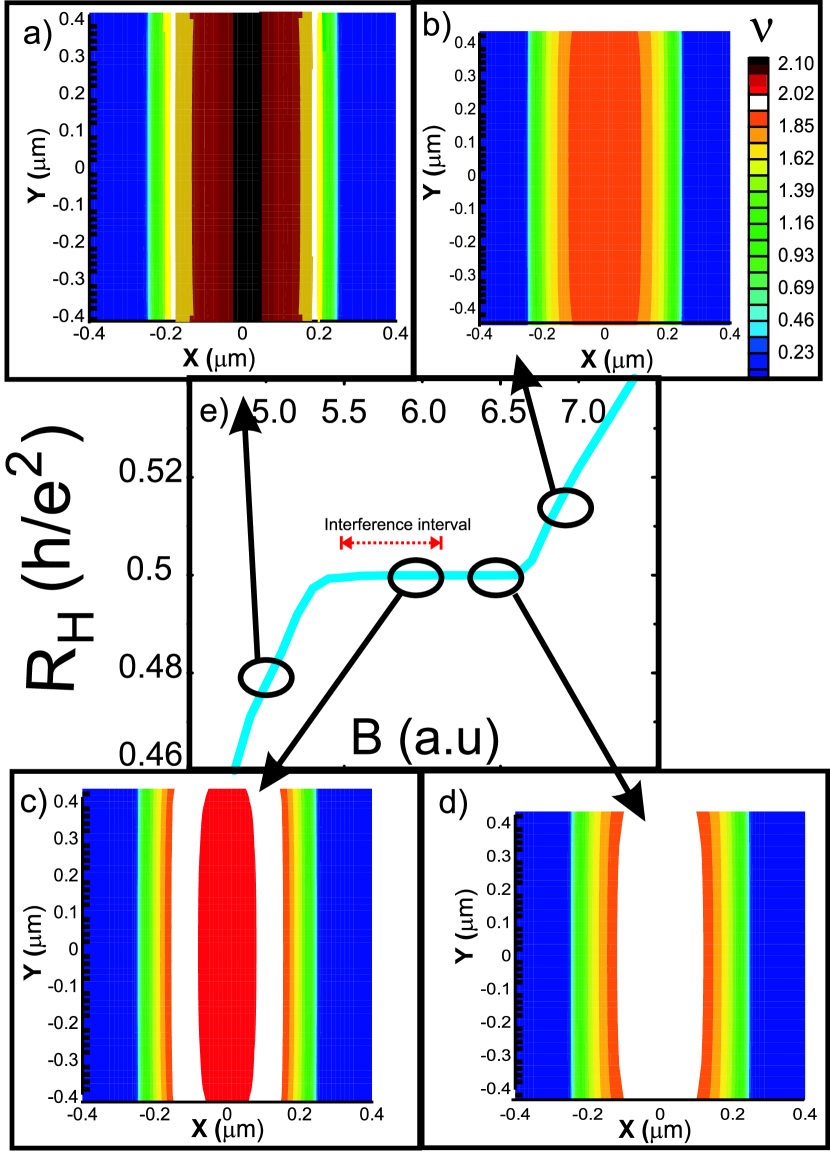
Figure 6: [a]-[d] Color-coded plot of the local filling factor versus position $(x,y)$ for a square sample of width $a_{x}=a_{y}=0.8\,\mu$m; white indicates $\nu(x,y)=2$. The average density is taken to be $3.0\cdot 10^{11}\,$cm^-2; $k_{B}T/E_{F}=0.02$. [e] A sketch of the Hall resistance as a function of magnetic field

Once the initial values of the screened potential and the electron distribution have been obtained for $T=0,B=0$, using the scheme described above, one can calculate these quantities for finite field and temperature as follows: replace the zero temperature Fermi function with the finite temperature one and insert the bare Landau DOS

$$D_{B}(E)=\frac{1}{\pi l_{b}^{2}}\sum_{n=0}^{\infty}{\delta(E-E_{n})},\quad E_{n}=\hbar\omega_{c}(n+1/2)$$ (12)

into equation (3) instead of $D_{0}$. In our numerical scheme we first start with relatively high temperatures (i.e. a smooth Fermi function) and then decrease the temperature slowly until the desired temperature is reached. A Newton-Raphson method is used for the iteration process and at every iteration step the electro-chemical potential is checked to be constant.

Before proceeding with the investigation of the QPC geometry at $B>0$, we would like to make clear the relation between the quantum Hall plateaus and the existence of the incompressible strips following the arguments of Siddiki and Gerhardts Siddiki and Gerhardts (2004a). Fig. 6 presents the local filling factors of a relatively small Hall bar, together with an illustrative Hall resistance curve. At the high magnetic field side ((b), $\nu(0,0)<2$) there are no incompressible strips, thus the system is out of the Hall plateau. When approaching from the high $B$ side to the plateau a single incompressible strip at the center develops. When the width of this strip becomes larger than the Fermi wavelength, the system is in the quantum Hall state ((d), $\nu(0,0)=2$). If we decrease the field strength further the center incompressible strip splits into two and moves toward the edges ((c) $\nu(0,0)>2$). As long as the widths of these strips are larger or comparable with the Fermi wavelength the system remains in the plateau. This is the regime in which an interferometer may be realized. Further decreasing the magnetic field leads to narrower incompressible strips which finally disappear if the widths of them become smaller than the average electron distance. Then the system leaves the quantized plateau. The distribution of the incompressible strips and the onset of the plateaus, of course, depends on the disorder potential Siddiki and Gerhardts (submitted to Int. J. Mod. Phys. B) and the physical size of the sample. However, the experiments considered here are done using narrow and high mobility structures, thus the above scheme will cover the experimental parameters.

In this subsection we present some of our results obtained within the TFA using periodic boundary conditions, considering two different tip separations, while sweeping the magnetic field. First we will fix the gate potential to $V_{QPC}=-0.3$V and sweep the magnetic field for $\Delta y=100$nm, while keeping the electron number density, i.e. the Fermi energy, constant. Second we examine the potential profile for $\Delta y=300$nm and comment on the possible effects on the coherent transport properties.

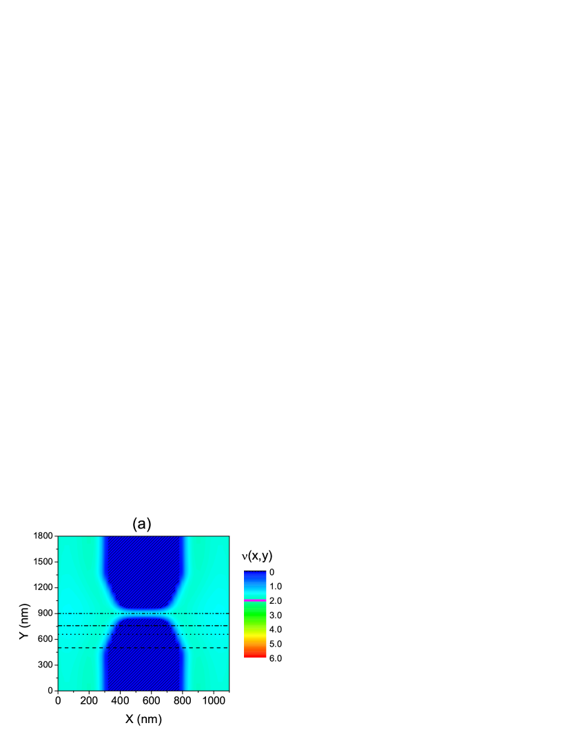
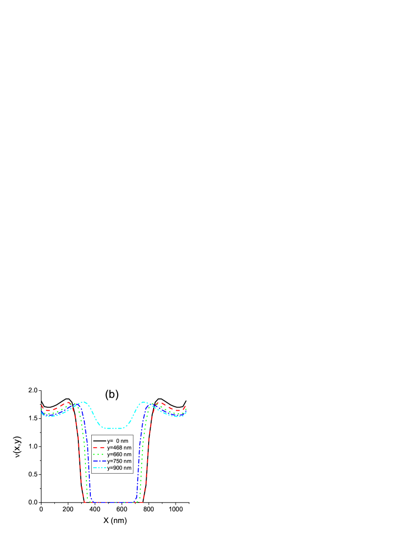
Figure 7: [a] The top view of the local filling factor, $\nu(x,y)$, distribution of the 2DES, for average filling factor one, in the plane located at $z=85$nm below the surface, at the ”default” temperature, $kT/\hbar\omega_{c}=1/50$, which will be used in all subsequent plot. The color scale depicts the density of electrons, whereas the dark shaded areas indicate the electron depleted regions. [b] Side view of the local filling factor for $y=0$nm(solid line), 468nm (dashed line), 660nm (dotted line), 750nm (dash-dotted line) and 900nm (dash-dotted-dashed line) . The horizontal lines in [a] shows the positions of the cuts in [b], with the same line code. Note that the density has local minima at large and small x, which are finite size effects mentioned in the text.

In figure 7 we plot the local filling factor (i.e. the normalized density) distribution of the 2DES projected on the $xy$-plane, together with the same quantity for some selected values of $y$, at average filling factor ($\bar{\nu}$) one. From the $y=0$nm curve (solid lines) in Fig.7[b], one can see that the electrons beneath the QPC are depleted (shaded, dark (blue) regions) ($300<x<800$nm), while the electron density reaches finite values while approaching the opening of the QPC ($y\sim 850$nm). At $\bar{\nu}=1$ one does not observe any incompressible regions, since the Fermi energy is pinned to the lowest Landau level. Hence the electron distribution is rather smooth and the current distribution will just be proportional to the number of electrons, similar to the Drude approach. For this case the external potential is screened almost perfectly and the self-consistent potential is almost flat, thus one can assume that the corresponding local wave functions are very similar to the ground state Landau wave functions.

The first incompressible region occurs when the Fermi energy falls in the gap between two low-lying Landau levels. Then the electrons exhibit a constant density and thus cannot screen the external potential. In figure (8)a, we show the electron distribution for $\bar{\nu}=1.1$. The black regions denote a local density corresponding to filling factor $\nu=2$, which does not percolate from the left side of the sample (which we might identify with the source) to the right side (drain). Here one can see well developed incompressible puddles, at the regions $150$nm$<x<250$nm, $0$nm$<y<450$nm (and four other symmetric ones) and two smaller puddles at the entrance of the QPC. These structures will remain unchanged even if one considers a larger unit cell, since they manifest the $q$- dependency, i.e. the rapid oscillations of the Fourier transform of the confining potential of the QPC.

In these regions the self-consistent potential exhibits a finite slope. Accordingly the wave functions will be shifted and squeezed, i.e. they are now superpositions of a few high order Landau wave functions with re-normalized center coordinates. This behavior has been shownSuzuki and Ando (1993); Siddiki and Gerhardts (2004a) for the translationally invariant model. Here we did not include the finite extent of the wave functions, here to avoid lengthy numerical calculations.

The incompressible regions shift their positions on the $xy$ plane depending on the strength and the profile of the confining potential. In figure (8)b we show the filling factor distribution where the bulk filling factor is almost two. We see that four incompressible strips are formed near the QPC. However the QPC opening remains in a compressible state, with local filling factor less than two, where we expect that the self-consistent potential is essentially flat. Further increasing the average filling factor, we observe that the bulk becomes completely compressible and two incompressible strips are formed near the QPC which percolate from bottom to top, creating a potential barrier with a height of $\hbar\omega_{c}$, see Fig. (8c). For even higher filling factors, they merge at the center of the QPC (Fig. 8d). In that case, the potential within the QPC will then no longer be flat, due to poor screening. We should also note that for a small width $\Delta y$ of the QPC opening, merging of the incompressible strips will happen only in a very narrow $B$ interval, and a quantitative evaluation within our TFA can not be always satisfactory, as the number of electrons inside the QPC becomes too low. Further decreasing the field strength (increasing the average filling factor) results in two separate incompressible strips winding around the opposite gates making up the QPC, as shown in Fig. 8e. Thus, dissipationless transport through the QPC, with a quantized conductance, becomes possible. At the lowest field values considered in this figure, we see that the innermost incompressible strips (with $\nu=2$) become smaller than the Fermi wavelength and thus they essentially disappear and no longer affect the transport properties. This point has been discussed in detail in a recent work by Siddiki et al.Siddiki and Gerhardts (2004a). The scheme described above now starts to repeat, but with incompressible strips having a local filling factor of 4.

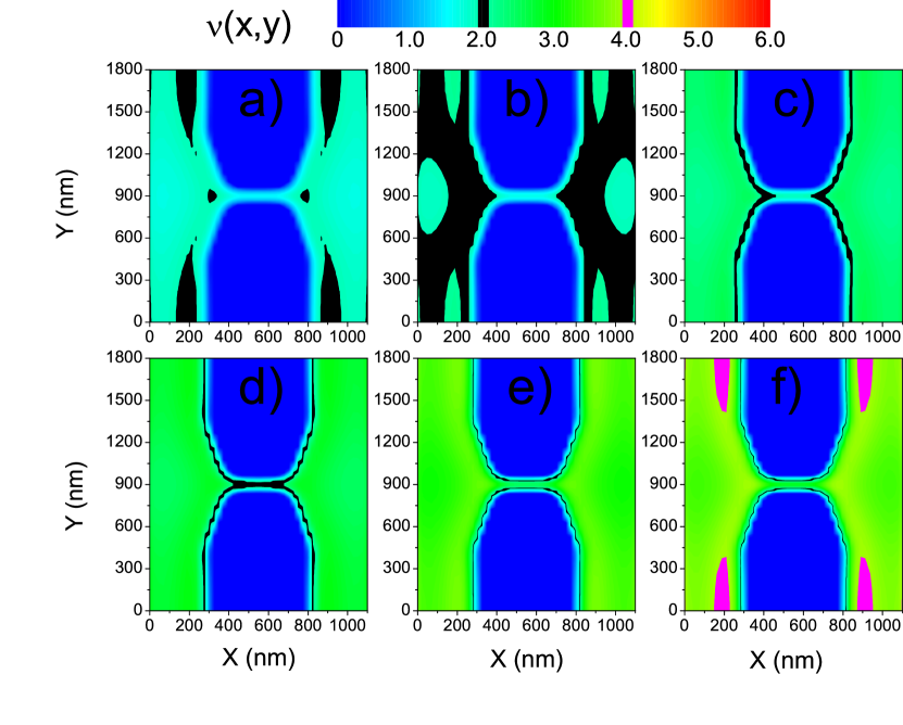
Figure 8: The local filling factor distribution for different average filling factors ($\bar{\nu}$), which is defined by the number of the electrons in the unit cell. [a] $\bar{\nu}=1.1$ [b] $1.2$ [c] $1.4$ [d] $1.6$ [e] $1.8$ [f] $2.2$. The color scale depicts the local electron concentration, whereas the abrupt colors indicate the even-integer filling factors, i.e. incompressible strips, (black for $\nu(x,y)=2$, magenta for $\nu(x,y)=4$.

We now discuss the effects of increasing the separation parameter, which we choose to be $\Delta y=300$nm in figure (9). At the strongest magnetic field (9a), only very small regions are incompressible and the electron distribution is similar to Fig.8a, where the incompressible regions result from local unpinning of the Fermi energy from the lowest Landau level due to $q-$dependent screening, i.e the shoulder-like variation of the potential near the QPC discussed earlier. By decreasing $B$, an interesting structure is observed at the center of the QPC: an incompressible island. In figure 9b, we have tuned the magnetic field such that the bulk of the 2DES is incompressible, meanwhile the entrance to the QPC remains compressible. The strong variation of the self-consistent potential at the center of the QPC can generate a pronounced effect on the current passing through the QPC (see figure 10 and the related text). For a lower magnetic field strength the distribution of the incompressible region is just the opposite (c). Now we see a large compressible puddle at the center, surrounded by incompressible regions, which can percolate from source to drain. Coherent, dissipationless transport can be expected in this case. Further decreasing the magnetic field we observe that the structure is smeared out and the tip region becomes compressible, nevertheless there are two large incompressible regions close to the entrance of the opening. The two incompressible strips wind around the gates, as shown in Fig. 9d. Finally, a scheme similar to that observed earlier in figure 8d-e is also seen now, for $\Delta y=300$nm.

Another remark which we would like to make concerns the edge profile of the sample itself and of the QPC. It has been shown both experimentallyHuber et al. (2005) and theoreticallyWulf et al. (1988); Siddiki and Gerhardts (2004a) that for an (almost) infinite potential barrier at the edges of the sample, the Chklovskii [Chklovskii et al., 1992] edge state picture breaks down, i.e. no incompressible strips near the edge can be observed. Meanwhile for smoothly varying edge potential profiles many incompressible strips are present, if the bulk filling factor is larger than two (for spinless electrons: four). We believe that, within the MZI setup both of these edge potential profiles might co-exist. At the edge regions of the sample, where lateral confinement is defined by physical etching, the potential profile differs from of the one generated by the top gates, due to different separation thicknesses and also lateral surface charges generated by etching. In principle gate and etching defined edges impose different boundary conditions, and the effects on screening at a 2DES have been discussed beforeSiddiki and Gerhardts (2003). These two profiles will certainly affect the group velocity, since the slope of the potential depends on the (lateral) boundary conditions. Following the arguments of Ref.[Güven and Gerhardts, 2003; Siddiki and Gerhardts, 2004a], which essentially predict that the dissipative current is confined to the incompressible strips, the widths of these strips will also define the slope, hence the velocity of the electrons will be determined by the edge profile. The velocity of the edge electrons were investigated experimentallyKarmakar et al. (to appear in Physica E, 2006) and the magnetic field dependency was reported as $B^{3/2}$. There it was noted that a self-consistent treatment is necessary to understand their findings, which we would like to discuss in a future publication.

The important features to note in these results are (i) in general, electron-electron interactions have a remarkable effect, leading to the formation of a local extremum in the potential at the center of the QPC, which even at low electron densities seems to be well described by the TFA; (ii) the narrow compressible/incompressible strips formed near the QPC are a direct consequence of the $q-$dependent screening.

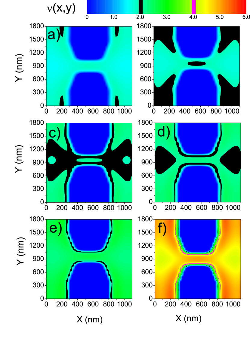
Figure 9: The local filling factor distribution for different average filling factors ($\bar{\nu}$), for a tip separation $\delta y=300$ nm. Note that, the number of electrons in the unit cell is changed, since the depleted areas are larger than of the previous figure. [a] $\bar{\nu}=1.14$ [b] $1.2$ [c] $1.34$ [d] $1.4$, [e] 1.6 and [g] 3.1. The color scale depicts the local electron concentration, whereas the high-contrast color regions indicate the even-integer filling factors, i.e. incompressible strips, (black for $\nu(x,y)=2$, magenta for $\nu(x,y)=4$). The calculations are done at $k_{B}T/\hbar\omega_{c}=1/50$ for an average electron density $1.7\times 10^{-11}cm^{-2}$.

IV.5 Comments on coherent transport

A complete calculation of coherent transport requires a deeper analysis of the wave functions and is beyond the scope of this work, which has been devoted to self-consistent realistic calculations of the potential and density profiles. In principle, one can follow the arguments of the well developed recursive Green’s function techniqueSols et al. (1989) in the absence of magnetic field and the method developed recently even in the presence of a strong fieldRotter et al. (2003).

Instead we would like to examine the potential distribution across the QPC and comment on the possible effects of interaction on the wave functions, and thereby (indirectly) on transport. In figure 10, we depict the potential profile across the QPC for the parameters used to obtain figure 8. As expected for $\bar{\nu}=1.0$ (dashed (red) line) the 2DES is ”quasi” metallic, hence the external potential is perfectly screened, and the wave functions are left almost unchanged. The two incompressible islands seen at the entrance of the QPC in Fig.8a lead to a minor variation of the screened potential at $x=300$nm and $x=800$nm, depicted by the solid (black) line for $\bar{\nu}=1.1$. A drastic change is observed when the bulk becomes incompressible ($\bar{\nu}=1.2$) and the opening remains compressible: Now the 2DES cannot screen the external potential near the openings of the QPC, where we see a strong variation. The strong perpendicular magnetic field changes the potential profile near the QPC via forming incompressible strips, and local minima are observed at the entrance and the exit. In these regions the electrons are strongly localized and the wave functions are squeezed. The situation is rather the opposite for $\bar{\nu}=1.4$, where two incompressible strips located near the QPC, formed due to $q$-dependent screening, merge at the opening. One observes a barrier with the height of $\hbar\omega_{c}$, which essentially is a direct consequence of the incompressible strip at the center and electrons have to overcome this barrier. Further decreasing the magnetic field smears out the barrier gradually, until the system becomes completely compressible and we are back in the case of figure 10a (also with regard to the transport properties).

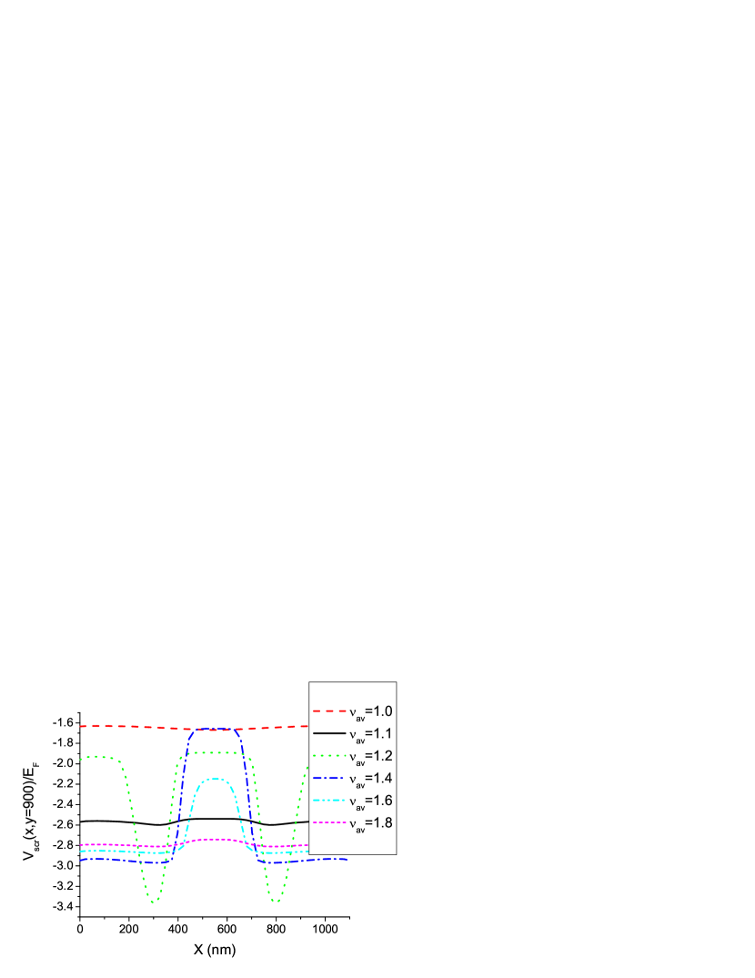
Figure 10: The self-consistent potential profile across the QPC, plotted for characteristic values of the average filling factor. Calculations are done at the default temperature and electron density.

V Summary

The study that motivated the present authors was the Quantum Hall effect based Mach-Zender interferometerJi et al. (2003); Neder et al. (2006). There are puzzles in the experiment for which it is not obvious (at least to us and some others) how they could be explained using scattering theory. Therefore we probably need to take into account interactions more seriously, including correlation effects in non-equilibrium transport that will not be part of scattering theory. A first step towards that goal then is the self-consistent mean-field equilibrium calculation which we have done.

At the moment we do not have to offer a non-equilibrium transport theory based on these equilibrium calculations. These effects may include decoherence due to potential fluctuations brought about by electron-electron or electron-phonon interactions (together with other noise sources). A more detailed understanding of electron-electron interactions in this setup, as well as of those features of the interferometer that are specific to the physics of the Quantum Hall effect, hinges on an analysis of the self-consistent static potential landscape near the QPCs, which represent the most crucial components of the setup.

Therefore, in this work, we have taken into account the electron-electron interaction within the TFA, considering realistic geometries of QPCs, calculating the self-consistent potential and electronic density profiles, and commenting on possible effects on transport.

The outcome of our model calculations can be summarized as follows: (i) We have obtained the electrostatic potential profile for the QPC geometries used in the experiments by solving the Laplace equation semi-analytically. (ii) We have demonstrated for a simple square well barrier that the screened potential in a 2DES, even in the absence of a magnetic field, is strongly dependent on the initial potential profile and on the distance between gates and 2DES. (iii) The screened potential has been calculated within the TFA for a QPC at vanishing field, where we have observed two interesting features: a local extremum at the center of the QPC and strong shoulder-like variations near the QPC. (iv) In the presence of a magnetic field, the formation and the evolution of the incompressible regions has been examined and three different cases have been observed: (a) the system is completely compressible. (b) An incompressible region and/or strip, which does not percolate from source to drain, generates a local extremum at the entrance/exit of the QPC (c) The center of the QPC becomes incompressible, with or without a compressible island, hence the incompressible strip percolates from source to drain. We note that the local minimum found at the center of the QPC for certain tip separations, being a clear interaction effect, coincides with the findings of Hirose et al [Hirose et al., 2003].

This work was partially supported by the German Israeli Project Cooperation (DIP) and by the SFB 631. One of the authors (A.S) would like to acknowledge R.R. Gerhardts, for his supervision, support and discussions, J. von Delft for offering the opportunity to work in his distinguished group and S. Ludwig for discussions on the experimental realization of QPC structures.

References

- van Wees et al. (1988) B. J. van Wees, H. van Houten, C. W. J. Beenakker, J. G. Williamson, L. P. Kouwenhoven, D. van der Marel, and C. T. Foxon, Phys. Rev. Lett 60, 848 (1988).
- Wharam et al. (1988) D. A. Wharam, T. J. Thornton, R. Newbury, M. Pepper, H. Ahmed, J. E. F. Frost, D. G. Hasko, D. C. Peacockt, D. A. Ritchie, and G. A. C. Jones, J. Phys. C 21 (1988).
- Thomas et al. (1996a) K. J. Thomas, J. T. Nicholls, M. Y. Simmons, M. Pepper, D. R. Mace, and D. A. Ritchie, Phys. Rev. Lett. 77, 135 (1996a).
- Thomas et al. (1996b) K. Thomas, J. Nicholls, M. Simmons, M. Pepper, D. Mace, and D. Ritchie, Phys. Rev. Lett. 77, 135 (1996b).
- Khrapai et al. (submitted to Phys. Rev. Lett) V. Khrapai, S. Ludwig, J. Kotthaus, and W. Wegscheider, cond-mat/0606377 (submitted to Phys. Rev. Lett).
- Ji et al. (2003) Y. Ji, Y. Chung, D. Sprinzak, M. Heiblum, D. Mahalu, and H. Shtrikman, Nature 422, 415 (2003).
- Neder et al. (2006) I. Neder, M. Heiblum, Y. Levinson, D. Mahalu, and V. Umansky, Phys. Rev. Lett. 96, 016804 (2006).
- Fiori et al. (2002) G. Fiori, G. Iannaccone, and M. Macucci, Journal of Computational Electronics 1, 39 (2002).
- Hirose et al. (2003) K. Hirose, Y. Meir, and N. S. Wingreen, Phys. Rev. Lett. 90, 026804 (2003).
- Reilly et al. (submitted to Physica E) D. J. Reilly, Y. Zhang, and L. DiCarlo, cond-mat/0601135 (submitted to Physica E).
- Seelig and Büttiker (2001) G. Seelig and M. Büttiker, Phys. Rev. B 64, 245313 (2001).
- Marquardt and Bruder (2004a) F. Marquardt and C. Bruder, Phys. Rev. Lett. 92, 056805 (2004a).
- Marquardt and Bruder (2004b) F. Marquardt and C. Bruder, Phys. Rev. B. 70, 125305 (2004b).
- Förster et al. (2005) H. Förster, S. Pilgram, and M. Büttiker, Phys. Rev. B. 72, 075301 (2005).
- Marquardt (2005) F. Marquardt, Europhys. Lett. 72, 788 (2005).
- Marquardt (2006) F. Marquardt, cond-mat/0604458 (2006).
- Pilgram et al. (2005) S. Pilgram, P. Samuelsson, H. Förster, and M. Büttiker, cond-mat/0512276 (2005).
- Marquardt (to be published in: ,,Advances in Solid State Physics”, Vol. 46, ed. R. Haug, Springer 2006) F. Marquardt, cond-mat/0604626 (to be published in: ,,Advances in Solid State Physics”, Vol. 46, ed. R. Haug, Springer 2006).
- v. Klitzing et al. (1980) K. v. Klitzing, G. Dorda, and M. Pepper, Phys. Rev. Lett. 45, 494 (1980).
- Ahlswede et al. (2002) E. Ahlswede, J. Weis, K. von Klitzing, and K. Eberl, Physica E 12, 165 (2002).
- Ilani et al. (2000) S. Ilani, A. Yacoby, D. Mahalu, and H. Shtrikman, Phys. Rev. Lett. 84, 3133 (2000).
- Güven and Gerhardts (2003) K. Güven and R. R. Gerhardts, Phys. Rev. B 67, 115327 (2003).
- Chklovskii et al. (1992) D. B. Chklovskii, B. I. Shklovskii, and L. I. Glazman, Phys. Rev. B 46, 4026 (1992).
- Siddiki and Gerhardts (2003) A. Siddiki and R. R. Gerhardts, Phys. Rev. B 68, 125315 (2003).
- Siddiki and Gerhardts (2004a) A. Siddiki and R. R. Gerhardts, Phys. Rev. B 70, 195335 (2004a).
- Siddiki and Gerhardts (2004b) A. Siddiki and R. R. Gerhardts, Int. J. Mod. Phys. B 18, 3541 (2004b).
- Büttiker (1988) M. Büttiker, IBM J. Res. Dev. 32, 317 (1988).
- Suzuki and Ando (1993) T. Suzuki and T. Ando, J. Phys. Soc. Jpn. 62, 2986 (1993).
- Ihnatsenka and Zozoulenko (2006) S. Ihnatsenka and I. V. Zozoulenko, Phys. Rev. B 73, 155314 (2006).
- Siddiki and Gerhardts (submitted to Int. J. Mod. Phys. B) A. Siddiki and R. R. Gerhardts, cond-mat/0608541 (submitted to Int. J. Mod. Phys. B).
- Ando et al. (1982) T. Ando, A. B. Fowler, and F. Stern, Rev. Mod. Phys. 54, 437 (1982).
- Ahlswede et al. (2001) E. Ahlswede, P. Weitz, J. Weis, K. von Klitzing, and K. Eberl, Physica B 298, 562 (2001).
- Siddiki (submitted to Phys. Rev. B) A. Siddiki, cond-mat/0608736 (submitted to Phys. Rev. B).
- Siddiki et al. (2006) A. Siddiki, S. Kraus, and R. R. Gerhardts, Physica E 34, 136 (2006).
- Tutuc et al. (2003) E. Tutuc, R. Pillarisetty, S. Melinte, E. DePoortere, and M. Shayegan, Phys. Rev. B 68, 201308 (2003).
- Pan et al. (2004) W. Pan, J. Reno, and J. Simmons, cond-mat/0407577 (2004).
- Davies et al. (1995) J. H. Davies, I. A. Larkin, and E. V. Sukhorukov, J. Appl. Phys. 77, 4504 (1995).
- Huettel et al. (to be submitted to Phys. Rev. B) A. K. Huettel, A. Siddiki, K. Eberl, and S. Ludwig (to be submitted to Phys. Rev. B).
- Oh and Gerhardts (1997) J. H. Oh and R. R. Gerhardts, Phys. Rev. B 56, 13519 (1997).
- Morse and Feshbach (1953) P. M. Morse and H. Feshbach, Methods of Theoretical Physics, vol. II (McGraw-Hill, New York, 1953), p. 1240.
- Stern (1967) F. Stern, Phys. Rev. Lett. 18, 546 (1967).
- Wulf et al. (1988) U. Wulf, V. Gudmundsson, and R. R. Gerhardts, Phys. Rev. B 38, 4218 (1988).
- Siddiki (2005) A. Siddiki, Ph.D. thesis, Julius-Maximilians-University Wurzburg (2005).
- (44) I. Neder, private communication.
- Huber et al. (2005) M. Huber, M. Grayson, M. Rother, W. Biberacher, W. Wegscheider, and G. Abstreiter, Phys. Rev. Lett. 94, 016805 (2005).
- Karmakar et al. (to appear in Physica E, 2006) B. Karmakar, G. H. Dohler, and B. M. Arora, cond-mat/0505282 (to appear in Physica E, 2006).
- Sols et al. (1989) F. Sols, M. Macucci, U. Ravaioli, and K. Hess, J. Appl. Phys. 66, 3892 (1989).
- Rotter et al. (2003) S. Rotter, B. Weingartner, N. Rohringer, and J. Burgdoerfer, Phys. Rev. B 68, 165302 (2003).