Granular systems Kinetic theory Porous material; granular materials

The rich behavior of the Boltzmann equation for dissipative gases

Abstract

Within the framework of the homogeneous non-linear Boltzmann equation, we present a new analytic method, without the intrinsic limitations of existing methods, for obtaining asymptotic solutions. This method permits extension of existing results for Maxwell molecules and hard spheres to large classes of particle interactions, from very hard spheres to softer than Maxwell molecules, as well as to more general forcing mechanisms, beyond free cooling and white noise driving. By combining this method with numerical solutions, obtained from the Direct Simulation Monte Carlo (DSMC) method, we study a broad class of models relevant for the dynamics of dissipative fluids, including granular gases. We establish a criterion connecting the stability of the non-equilibrium steady state to an exponentially bound form for the velocity distribution $F$, which varies depending on the forcing mechanism. Power laws arise in marginal stability cases, of which several new cases are reported. Our results provide a minimal framework for interpreting large classes of experiments on driven granular gases.

Granular materials are ubiquitous in natural phenomena and widely used in industrial processes. Yet, a fundamental understanding of their properties still challenges scientists [1, 2]. Although a large number of particles is involved, a thermodynamic-like description remains elusive and has been thwarted by energy losses through internal dissipation, and energy supplies from non-thermal sources. Granular media are therefore intrinsically far from equilibrium, and a paradigm for open dissipative systems. One can distinguish two types of granular fluids [1]: quasi-static flows (solid-like), where gravity, friction and stress distributions control the dynamics, and rapid granular flows (gas-like), where the dynamics is mostly governed by ballistic motion in between inelastic collisions. This letter deals with granular gases.

Even dilute granular gases differ from their molecular counterparts to a significant extent [1, 2], and their particle velocity distribution is emblematic of the difficulties of a statistical description. The experimentally measured velocity distribution $F({\bf v})$ generically deviates from the Maxwell-Boltzmann behavior, and its functional form –often fitted by stretched exponentials– depends on material property, on the specific geometry considered and on the forcing mechanism which compensates the collisional loss of energy [3, 4, 6, 5, 7]. A similar picture emerges from numerical simulations and analytical studies [5, 8, 9, 10, 11, 12, 13, 14, 15, 16, 17, 18, 19, 20, 21, 22, 23, 24, 25], where in addition to the more common stretched exponential behavior, power-law distributions have also been reported [16, 17, 25]. This rather vast but disparate body of knowledge calls for rationalization.

Our goal is to propose a general and unified framework for interpreting experimental results, as well as to generalize existing theoretical results in two new and important directions: (i) to more general repulsive interactions, parametrized by an exponent $\nu$ , which include the known results for Maxwell molecules $(\nu=0)$ and hard spheres ($\nu=1$), and (ii) to more general forcing mechanisms, such as nonlinear negative friction forces, parametrized by an exponent $\theta$, including free cooling ($\theta=1$), as well as the white noise driving force. In addition, since the Maxwell-Boltzmann distribution seems to have no analog in steady states of dissipative gases, we want to identify the generic trends for the velocity distribution and study its properties in this framework. To this aim, we develop a global and quantitative cartoon of the different effects at work, that lead, upon changing certain key parameters, to the wide range of behaviors alluded to above.

In this letter, we develop a new analytic method for determining deviations from Gaussian behavior, that is free of the intrinsic limitations of previous approaches. For instance, the known Fourier transform method for obtaining high energy power law tails [27, 16, 17] is intrinsically restricted to Maxwell molecules, where the nonlinear collision term is a convolution product. Moreover, the method for obtaining stretched exponential tails in [11, 17] was based on a one-stroke asymptotic approximation, whereas our new method provides a systematic approximation scheme yielding large sub-leading corrections. We also show that the large velocity tail of $F(\mathbf{v})$ is characterized by an exponent $b$, which governs the stability of the non-equilibrium steady state. When this state is a stable fixed point of the dynamics, $b>0$ and $F$ is of stretched exponential form $\sim\exp[-v^{b}]$. We also emphasize the relevance of subdominant corrections that must be taken into account for a comparison of numerical or experimental data with the theory. For cases of marginal stability where $b$ vanishes, new classes of power law tails $v^{-s}$ appear. An immediate experimental consequence is that such power law tails will be elusive, since they can only arise when material properties are fine tuned. Small variations will either drive the system into an unstable state, or into a stable state with a stretched exponential tail.

We use the simplest model for rapid granular flows, i.e. the nonlinear Boltzmann equation, that corresponds to a regularly ’randomized’ gas (by shaking, fluidization, vibrational techniques, or bulk driving through alternating electric fields). The dynamics is described as a succession of uncorrelated inelastic binary collisions, modelled by soft spheres with collision frequency, $g\varsigma(g,\vartheta)\sim g^{\nu}|\widehat{\mathbf{g}}\cdot\bf{n}|^{\sigma}$, and a coefficient of normal restitution $\alpha<1$. The collision law $(\mathbf{v}_{1},\mathbf{v}_{2})\to(\mathbf{v}^{\prime}_{1},\bf v^{\prime}_{2})$ reads: $\mathbf{v}^{\prime}_{1}=\mathbf{v}_{1}-p(\bf{g}\!\cdot\!\bf{n})\bf{n}$ where $\bf{g}\equiv\mathbf{v}_{1}-\mathbf{v}_{2}$, $p=1-q=\frac{1}{2}(1+\alpha)$ and $\bf{n}$ is a unit vector parallel to the impact direction connecting particles 1 and 2. The expression for $\mathbf{v}^{\prime}_{2}$ follows from momentum conservation. Momentum transfer at a distance can also take place through long range interactions [4, 5]. Collisions dissipate kinetic energy at a rate $\propto{1\over 2}(1-\alpha^{2})=2pq$. The quantity $\varsigma(g,\vartheta)$ is the differential scattering cross section, where exponent $\sigma$ models the angular dependence, and $\mathbf{\widehat{g}}={\bf g}/g$ is a unit vector, parallel to $\bf{g}$. For elastic particles interacting via a soft sphere potential $U(r)\propto r^{-a}$, one has $\nu=1-2(d-1)/a$, where $d$ is the space dimension. The exponents $\nu=\sigma=1$ model ordinary hard-sphere behavior $(a\to\infty)$, and $\nu=0$ defines so-called Maxwell models. The hallmark of Maxwell interactions is a collision frequency independent of the relative velocity of the colliding pair. In Ref.[5] this property has been found experimentally, and explained theoretically for experiments on non-magnetic particles in a viscous fluid, and magnetic grains with dipolar interactions in air in a 2-D geometry where $U(r)=r^{-2}$. Because of this hallmark property, Maxwell models are particularly convenient for analytical purposes. Note also that the importance of material properties has barely been taken into account in previous studies. Here we do so in a necessarily schematic but physically relevant manner through the parameters $\nu$, $\sigma$ and $\alpha$, that encode material properties.

The study of the homogeneous systems is not only a useful starting point, it is also relevant to experiments with bulk driving [6, 5], and a significant fraction of the experiments [3, 4, 5, 6, 7] has been carried out on spatially uniform systems. The homogeneous non-linear Boltzmann reads

$$\partial_{t}F({\mathbf{v}},t)+{\cal F}F=\int^{\prime}d{\mathbf{v}}_{1}d{\mathbf{v}}_{2}d\bf{n}\,g^{\nu}|\widehat{\bf{g}}\cdot{\bf{n}}|^{\sigma}F({\mathbf{v}}_{1},t)F({\mathbf{v}}_{2},t)[\delta(\mathbf{v}-\mathbf{v}^{\prime}_{1})-\delta(\mathbf{v}-\mathbf{v}_{1})],$$ (1)

where the r.h.s defines the collision kernel $I(\mathbf{v}|F)$ with the usual gain/loss structure and Dirac functions to enforce the collision law; $\int^{\prime}$ indicates that the $\bf{n}$ -integration is an average over the pre-collision hemisphere, $\mathbf{g}\cdot\bf{n}\leq 0$, with a uniform weight normalized to unity. The forcing term ${\cal F}F$ represents the energy supply. We consider here the generic form

$${\cal F}F\,=\,\gamma\,\partial_{\mathbf{v}}\cdot({\mathbf{v}}v^{\theta-1}F)\,-\,D\,\partial_{{\mathbf{v}}}^{2}F$$ (2)

with either ($\gamma=0$, $D>0$) or ($\gamma>0$, $D=0$), corresponding respectively to stochastic White Noise (WN), or deterministic nonlinear Negative Friction (NF), where $\theta\geq 0$ is a continuous exponent. The change in velocity due to the latter force is proportional to $v^{\theta-1}{\mathbf{v}}$. For instance, for $\theta>1$ it injects selectively energy in the high energy tail of $F(v)$. A physical realization of NF with $\theta>1$ is provided by an electrically forced gas with a charge distribution. Energy is predominantly injected in the particles with a high charge, which in turn reach larger typical velocities. Recently a somewhat different device with a similar property has been proposed in Ref.[25]. The special case $\theta=1$ corresponds to the Gaussian thermostat [12], allowing to study the long time scaling regime of an unforced system (so-called free cooling), while $\theta=0$ models gliding friction, also called gravity thermostat [12]. It corresponds to a force of constant strength acting in the direction of the velocity. WN forcing has been frequently used in analytical and numerical studies [11, 12, 14, 19, 23], and more importantly, was shown to be experimentally relevant for two dimensional experiments with energy injected from a vibrating rough plate [6, 7]. In such cases individual grains undergo random changes in direction, that are mimicked by white noise forcing. Existing experimental evidence also shows that stochastic forcing is frequently a valuable first approximation [4, 14]. We therefore have a restricted ’phase space’ to explore:($\nu,\sigma,\alpha$) for WN and ($\nu,\sigma,\alpha,\theta$) for NF. Here $\gamma$ and $D$ are irrelevant constants that set the energy scale.

While the dynamics defined by (1) and (2) always admits a non-equilibrium steady state, the first question to address is the stability of this steady state. Our analysis assumes a rapid approach of $F$ to a scaling form $F(v,t)=(1/v_{0}(t))^{d}f(v/v_{0}(t))$ (for proofs, see [18]), where the r.m.s. velocity $v_{0}$ is defined through the granular temperature, $\int d{\bf v}v^{2}F(v,t)={1\over 2}dv_{0}^{2}(t)$, and Eq.(1) implies:

$$dv_{0}^{2}/dt\propto 1-\left(v_{0}(t)/v_{0}(\infty)\right)^{2b}\quad(b_{\rm{WN}}=1+\nu/2)$$

$$dv_{0}/dt\propto v_{0}^{\theta}(t)\left[1-\left(v_{0}(t)/v_{0}(\infty)\right)^{b}\right]\quad(b_{\rm{NF}}=1+\nu-\theta)$$ (3)

The solution $v_{0}$ therefore approaches the fixed point $v_{0}(\infty)$ if $b>0$, and conversely moves away from $v_{0}(\infty)$ if $b<0$, in which case the steady state is an unstable fixed point of the dynamics.

In stable steady states the integral equations for $f(c)$ can be derived from (1), and read for WN and NF driving respectively:

$$I(c|f)=-\frac{D}{(v_{0}(\infty))^{2b}}\partial^{2}_{{\bf c}}f=-\frac{\lambda_{2}}{4d}\langle\langle g^{\nu+2}\rangle\rangle\partial^{2}_{{\bf c}}f$$

$$I(c|f)=\frac{\gamma}{(v_{0}(\infty))^{b}}\partial_{{\bf c}}\!\cdot\!(\widehat{{\bf c}}c^{\theta}f)=\frac{\lambda_{2}\langle\langle g^{\nu+2}\rangle\rangle}{4\langle c^{\theta+1}\rangle}{\partial}_{{\bf c}}\!\cdot\!(\widehat{{\bf c}}c^{\theta}f)$$ (4)

The phenomenological constants $D$ and $\gamma$ have been eliminated with the help of the steady state conditions in ( The rich behavior of the Boltzmann equation for dissipative gases). The averages $\langle\langle\cdots\rangle\rangle$ and $\langle\cdots\rangle$ are respectively taken over the unknown $f(c_{1})f(c_{2})$ and $f(c)$, and $g=|\bf{c}_{1}-\bf{c}_{2}|$. Moreover $\lambda_{2}=2pq\beta_{\sigma+2}$ and $\beta_{s}\equiv\int d{\bf{n}}\>{\bf|\widehat{a}\cdot\bf{n}}|^{s}/\int{d}\bf{n}$ is an average of $|\cos\vartheta|^{s}$ over a $d$-dimensional solid angle.

Next we discuss the new criterion relating stretching exponents to stability. From the one stroke asymptotic approximation of [11] an interesting feature already emerges: in the stability region ($b>0$), $f(c)$ is of stretched exponential form with an a priori known exponent $b$ from ( The rich behavior of the Boltzmann equation for dissipative gases), while in cases of marginal stability ($b\to 0^{+}$), $f\sim c^{-a}$ is of power law type with an a priori unknown exponent $a$. As expected, $b$ decreases with $\nu$, since a tail particle with velocity $c\gg 1$ suffers collisions at a rate $c^{\nu}$; the slower the rate, the slower the particle redistributes its energy over the thermal range $c\stackrel{{\scriptstyle<}}{{\sim}}1$, which results in an increasingly overpopulated high energy tail. When $\nu$ is further decreased so that $b$ changes sign, the tail is no longer able to equilibrate with the thermal “bulk”, and the system cannot sustain a steady state. A similar intuitive picture may be developed with respect to $\theta$ in the NF cases. While $\theta=1$ is equivalent to a linear rescaling of velocities, a nonlinear rescaling with $\theta>1$ selectively puts more energy in the tail particles, thus leading to an increased overpopulation, as $b$ decreases (see ( The rich behavior of the Boltzmann equation for dissipative gases)). The reverse scenario applies for $\theta<1$.

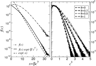
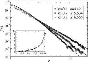
Figure 1: Comparison of the velocity distribution obtained from Monte Carlo simulations with the asymptotic predictions. Left: WN forcing for $d=2$, $\alpha=1/2$, $\sigma=\nu=-1/2$, where $b=3/4,b^{\prime}=9/16,\chi=0$. DSMC data are plotted as $f(c)$ (dashed-dotted line) and $\exp[-\beta^{\prime}c^{b^{\prime}}]f(c)$ (solid line) vs $x=\beta c^{b}$, and compared with the theoretical prediction $e^{-x}$ (dashed line). Right: NF forcing with $d=1$, $\alpha=0,\nu=1/2$. The DSMC data for $f(c)$ vs $c^{b}$ are compared at various $\theta$ with the prediction $\exp[-\beta c^{b}]$ (dashed lines). $\beta,\beta^{\prime}$ have been measured in the DSMC simulations from their definition (7). Fig.2: WN-driven system at stability threshold ($d=2,\nu=-2,\sigma=1$) for different values of the restitution coefficient $\alpha$. The dashed lines correspond to the theoretically predicted power-law tails $1/c^{a}$. The inset shows the algebraic exponent obtained through the numerical solutions of Eq.( The rich behavior of the Boltzmann equation for dissipative gases).

To be more specific, the collision operator $I$ in (1) for $c\gg 1$, acting on exponentially bound functions $f\sim\exp[-\beta c^{b}]$, reduces to a linear operator on $f$, because $\bf{g}\simeq\bf{c}_{1}$ and ${\bf{c}}^{\prime}_{1}\simeq{\bf{c}}_{1}-{p}(\bf{c}_{1}\cdot\bf{n})\bf{n}$, yielding the dominant behavior of Ref.[11], and a new important subleading correction [26],

$$I_{\infty}(c|f)=-\beta_{\sigma}c^{\nu}[1-{\mathcal{K}}_{\sigma}c^{-b(\sigma+1)/2}]f.$$ (5)

Here ${\mathcal{K}}_{\sigma}$ is non-vanishing, except for 1-D. Its explicit form contains averages $\langle\langle g^{s}\rangle\rangle$ and $\langle c^{s}\rangle$ [26]. The leading term is a direct generalization of the standard methods of Ref.[11] for inelastic hard spheres ($\nu=1$) and Maxwell molecules ($\nu=0$). Eq.(5) allows us to calculate for $c\gg 1$ sub-leading multiplicative corrections to $f(c)$ of the form,

$$\ln f(c)\sim-\beta c^{b}+\beta^{\prime}c^{b^{\prime}}+\chi\ln c+{\mathcal{O}}(1),$$ (6)

where $b>b^{\prime}>0$. By inserting (5)-(6) in ( The rich behavior of the Boltzmann equation for dissipative gases), and equating exponents and coefficients of the leading and sub-leading terms, we recover the $b-$values in ( The rich behavior of the Boltzmann equation for dissipative gases), and determine $\beta,b^{\prime},\beta^{\prime},\chi$. We only list the values for $\sigma=1$ (for further details, see [26]):

$$(\beta b)_{\rm WN}=\sqrt{d(d+1)/(pq\langle\langle g^{\nu+2}\rangle\rangle)}\ ;\ (\beta b)_{\rm NF}=(d+1)\langle c^{\theta+1}\rangle/(pq\langle\langle g^{\nu+2}\rangle\rangle)$$ (7)

which includes the special cases considered in Ref. [11]. Regarding the sub-leading quantities we find for $\sigma=1$, all values of $q=\frac{1}{2}(1-\alpha)$ and $d$,

$$\beta^{\prime}=0, \chi= -\textstyle{\frac{1}{4}}\nu-(d-1)q^{2}/2(1-q^{2})\quad(\mbox{WN})$$

$$\beta^{\prime}=0, \chi= -\theta+(d-1)q^{2}/(1-q^{2})\quad(\mbox{NF}).$$ (8)

For $\sigma>1$ we find sub-leading results similar to ( The rich behavior of the Boltzmann equation for dissipative gases) with $\chi_{\rm WN}=\frac{1}{2}(1-d)-\frac{1}{4}\nu$ and $\chi_{\rm NF}=1-d-\theta$. For $\sigma<1$ we obtain $b^{\prime}=\frac{1}{2}b(1-\sigma),\chi=0,\beta^{\prime}\propto\beta{\mathcal{K}}_{\sigma}$, both for WN and NF with corresponding values for $b$ and $\beta$. A striking example of the importance of the new sub-leading corrections is shown in Fig.1(left) for a model with $\sigma=-1/2$. The numerical results are obtained from the Direct Simulation Monte Carlo technique (DSMC), which offers an efficient algorithm to solve the nonlinear Boltzmann equation [28]. The dashed-dotted curve in Fig. 1(left) shows that the simulated $c-$values are not large enough to agree with the asymptotic predictions. However, the solid curve shows a striking agreement with the theory. This demonstrates the importance of the sub-leading corrections, which allow to extend the validity of the asymptotic theory to much smaller $c-$value, which are likely to be helpful in experimental verification. Such corrections are generic in dissipative gases for $d\leq 2$, and more pronounced when $\sigma<1$. In 1D they are absent (see Fig.1(right)).

Next we analyze the integral equation ( The rich behavior of the Boltzmann equation for dissipative gases) at the stability threshold ($b=0$), where power law tails, $f(c)\sim c^{-a}$, are to be expected. The asymptotic approximations, made in (5), are no longer valid because of the slow decay of $f(c_{2})$ in $I(c|f)$ at large velocities. Here we proceed as follows. As far as large velocities are concerned ($c\gg 1$), the thermal range of $f$ may be viewed to zeroth approximation as a Dirac delta function $\delta({\bf c})$, carrying all the mass of the distribution. We therefore write $f{(\bf{c})}=\delta{(\bf{c})}+h({\bf{c}})$, where $h$ represents the high energy tail, of negligible weight compared to the thermal bulk. This allows us to linearize the collision operator:

$$I({\bf{c}}|\delta+h)=-\Lambda h(c)+{\mathcal{O}}(h^{2}),$$ (9)

where we have used that $\delta(\bf{c})$ makes the nonlinear collision term vanish [$I(\bf{c}|\delta)=0$]. Hence, (9) defines the linearized collision operator $\Lambda$. Its eigenfunctions are of power law type, and particularly suited to describe the algebraic decay of $f$ in cases of marginal stability. For the construction of $\Lambda$, which differs from its self-adjoint $\Lambda^{\dagger}$, and of its eigenfunctions and eigenvalues we refer to [26]. For the special case of Maxwell molecules the eigenvalues of the linearized collision operator have been calculated in Refs.[27, 16, 17] with the help of the Fourier transform method, which can not be applied to non-Maxwell type interactions. The essential observation in deriving the spectral properties is that $\Lambda$, applied to any power $c^{a}$ generates a term $\propto c^{a+\nu}$. This property allows us to calculate the eigenvalues $\lambda_{s}$, and the corresponding left eigenfunctions, $\Lambda^{\dagger}c^{s}=$ $\lambda_{s}c^{s+\nu}$, and right ones, $\Lambda c^{-s-d-\nu}=$ $\lambda_{s}c^{-s-d}$. These spectral properties, including

$$\lambda_{s}\!=\!\beta_{\sigma}\left\{1-_{2}\!F_{1}\,\left(\textstyle{-\frac{s}{2},\frac{\sigma+1}{2};\frac{\sigma+d}{2}}\,|\,1-q^{2}\right)\right\}-p^{s}\beta_{s+\sigma},$$ (10)

are new results. Here ${}_{2}\!F_{1}$ is a hypergeometric function, $\lambda_{s}$ is well-defined for $s\geq 0$, and $\lambda_{0}=0$ is an isolated point of the spectrum. The eigenvalue depends only on the angular exponent $\sigma$, and not on the energy exponent $\nu$. Moreover, for $s=2$ one has $\lambda_{2}=2pq\beta_{\sigma+2}$ (see Eq.( The rich behavior of the Boltzmann equation for dissipative gases)). Consequently, in the threshold cases ($b=0$, which fixes the exponent $\nu$ at threshold to $\nu_{\rm WN}=-2$ or $\nu_{\rm NF}=\theta-1$) the asymptotic form of $f(c)$ is given by the right eigenfunction that satisfies the integral equation ( The rich behavior of the Boltzmann equation for dissipative gases). Substitution yields the transcendental equations:

$$\lambda_{s} = \textstyle{\frac{1}{4d}}s(s+d-2)\lambda_{2}\qquad({\rm WN})$$

$$\lambda_{s} = \textstyle{\frac{1}{2}}s\lambda_{2}\langle\langle g^{\theta+1}\rangle/\langle c^{\theta+1}\rangle\equiv\textstyle{\frac{1}{2}}s\lambda_{2}\Gamma(\theta)\>({\rm NF})$$ (11)

Their largest root $s^{*}$ determines the exponent of the corresponding high energy tail, $f(c)\sim 1/c^{s^{*}+d+\nu}$ for the different driving forces at their stability threshold ($b=0$).

For the Gaussian thermostat ($\theta=1$, $\Gamma(1)=1$) the threshold model ($b_{\rm NF}=\nu_{\rm NF}=0$) is the well-studied Maxwell model with a high energy tail, $f(c)\sim 1/c^{s^{*}+d}$, first discovered in Ref.[16, 17]. In the 1-D case (where $\beta_{s}=1$) the eigenvalue (10) simplifies to $\lambda_{s}=1-q^{s}-p^{s}$, and ( The rich behavior of the Boltzmann equation for dissipative gases) can be solved analytically for WN, yielding $s^{*}(d=1)=3$ and $f(c)\sim 1/c^{s^{*}+d-2}\sim 1/c^{2}$, as well as for NF $(\theta=1)$, yielding $s^{*}_{\rm NF}(d=1,\theta=1)=3$ and $f(c)\sim 1/c^{s^{*}+d+\theta-1}\sim 1/c^{4}$. For all remaining ($d,\theta$) values, ( The rich behavior of the Boltzmann equation for dissipative gases) can be solved numerically, where the ratio $\Gamma(\theta)$ is independently measured in the DSMC method. All power law exponents are found to be extremely accurate for all driving mechanism, for all values of the restitution coefficient $\alpha$, and for all dimensions (see Fig.2). So, a new class of power law tails is obtained for WN and NF friction.

Let us now discuss the power law tail generated by an energy source ’at infinity’, as recently proposed in Ref. [25] with suggestions for experimental tests. Here the source regularly injects a macroscopic amount of energy in the system at ultra high energies. This energy cascades down to lower energies, and builds up a stationary ’low’ energy tail $h(c)$. The mathematical framework developed in the present paper is also well suited to discuss this mechanism. By the arguments above (9) the collision operator can be linearized, and the tail distribution satisfies, $\Lambda h=0$. So we determine the right eigenfunction, $h\sim c^{s^{*}-d-\nu}$ with eigenvalue $\lambda_{s^{*}}=0$. As $\lambda_{s}(s\to 0^{+})=-1$, there does exist a non-vanishing positive solution $s^{*}(d,\sigma,\alpha)>0$. As shown in Ref. [26], the equation for $s^{*}$ is equivalent to the one solved in [25] for the soft sphere model ($\sigma=\nu$). In 1-D it has the analytic solution $s^{*}(d=1)=1$ and $h(c)\sim c^{-2-\nu}$. For $d>1$ the equation can been solved numerically. Also the more traditional thermostats, as discussed in the context of inelastic gases in Ref.[20], can be analyzed with the help of the present method [26].

In this Letter, we have studied a general class of inelastic soft sphere models, on the basis of the nonlinear Boltzmann equation coupled to stochastic or deterministic driving forces. We provide a general framework which embeds in a versatile description the majority of driving devices and of particle interactions, discussed in the literature: from hard scatterers like inelastic hard spheres to soft scatterers like Maxwell molecules; from driving by white noise, nonlinear friction, an energy source ”at infinity”, as well as by traditional thermostats. It therefore represents a minimal model for interpreting experiments on driven granular gases, discussing trends, etc. When the non-equilibrium steady state is an attractive fixed point of the dynamics, the velocity distribution $f(c)$ has a stretched exponential tail $\propto\exp(-c^{b})$; sub-leading corrections appear in certain regions of model parameters ($\nu,\alpha,\theta$), where $f(c)$ is found to be of the form $c^{\chi}\exp(-\beta v^{b}+\beta^{\prime}v^{b^{\prime}})$. These corrections turn out to be of particular relevance since they allow to obtain an agreement with asymptotical theoretical predictions in a much larger range of velocities, therefore more easily accessible to experiments. On the other hand, algebraic distributions emerge in cases of marginal stability ($b=0$), where power law exponents have been calculated. We have argued that such distributions should be extremely difficult to observe experimentally.

Our theoretical starting point is backed up by recent experimental findings, and all predictions –derived from a new analytical method– have been tested against very extensive Monte Carlo simulations [26]. Our work therefore calls for further experimental investigations; in particular, electrically forced gases with a charge distribution seem to provide interesting test-beds.

References

- [1] H.M. Jaeger, S.R. Nagel, and R.P. Behringer, Rev. Mod. Phys. 68, 1259 (1996);
- [2] I. Goldhirsch, Ann. Rev. Fluid Mech. 35, 267 (2003); Theory of Granular Gas Dynamics, Th. Pöschel and N.V. Brilliantov (Eds), (Springer-Verlag, Berlin, 2003).
- [3] J. S. Olafsen and J. S. Urbach, Phys. Rev. Lett. 81, 4369 (1998) and Phys. Rev. E 60, R2468 (1999); W. Losert et al, Chaos 9, 682 (1999); F. Rouyer and N. Menon, Phys. Rev. Lett. 85, 3676 (2000); D.L. Blair and A. Kudrolli, Phys. Rev. E 64, R050301 (2001).
- [4] I.S. Aranson, J.S. Olafsen, Phys. Rev. E66, 061302 (2002).
- [5] K. Kohlstedt, A. Snezhko, M.V. Sakozhnikov, I.S. Aranson, J.S. Olafson, E. Ben-Naim, Phys. Rev. Lett. 95, 068001 (2005).
- [6] A. Prevost et al, Phys. Rev. Lett. 89, 084301 (2002).
- [7] P. Melby et al, J. Phys.: Condens. Mat. 17, S2689, (2005).
- [8] A. Goldshtein, M. Shapiro, J. Fluid Mech.282, 75 (1995).
- [9] J.J. Brey et al, Phys. Rev. E58, 4200 (1998); Phys. Rev. E59 1256 (1999); J.J. Brey and M.J. Ruiz-Montero, Phys. Rev. E67, 021307 (2003).
- [10] A. Puglisi, et al, Phys. Rev. Lett. 81, 3848 (1998).
- [11] T.P.C. van Noije, M.H. Ernst, Gran. Mat.1, 57 (1998).
- [12] J.M. Montanero and A. Santos, Gran. Mat. 2, 53 (2000).
- [13] R. Cafiero, S. Luding and H.J. Herrmann, Phys. Rev. Lett. 84, 6014 (2000).
- [14] S.J. Moon et al, Phys. Rev. E 64, 031303 (2001).
- [15] A. Santos, J.W. Dufty, Phys. Rev. Lett. 86, 4823 (2001).
- [16] E. Ben-Naim, P.L. Krapivsky, Phys. Rev. E 61, R5 (2000); ibidem 66, 1309 (2002);
- [17] M.H. Ernst and R. Brito, Phys. Rev. E 65, 040301 (2002), and J. Stat. Phys. 109, 407 (2002).
- [18] A.V. Bobylev, C. Cercignani and G. Toscani, J. Stat. Phys. 111, 403 (2003); I.M. Gamba, V. Panferov and C. Villani, Comm. Math. Phys. 246, 503 (2004).
- [19] A. Barrat et al, J. Phys. A: Math. Gen. 35, 463 (2002).
- [20] Th. Biben et al, Physica A 310, 308 (2002); E. Barkai, J. Stat. Phys. 115, 1537 (2004).
- [21] D. ben-Avraham et al, Phys.Rev. E 68, 050103 (2003).
- [22] O. Herbst et al, Phys.Rev. E 70, 051313 (2004).
- [23] J.S. van Zon et al, Phys. Rev. E 72, 051301 (2005).
- [24] Y. Srebro, D. Levine, Phys. Rev. Lett. 93, 240601 (2004).
- [25] E. Ben-Naim, B. Machta and J. Machta, Phys. Rev. E 72, 021302 (2005); E. Ben-Naim and J. Machta, Phys. Rev. Lett. 94, 138001 (2005).
- [26] M.H. Ernst, E. Trizac and A. Barrat, to appear in J. Stat. Phys. (DOI: 10.1007/s10955-006-9062-6), and Proceedings Pucon Workshop Granular Materials, Dec. 2003, www.dfi.uchile.cl/swgm03 (see ’Contributions’, M.Ernst[zip]).
- [27] A.V. Bobylev et al, J. Stat. Phys. 98, 743 (2000).
- [28] G. Bird, Molecular Gas Dynamics and the Direct Simulation of Gas Flows (Clarendon, Oxford, 1994).