Self-consistent Coulomb picture of an electron-electron bilayer system

Abstract

In this work we implement the self-consistent Thomas-Fermi approach and a local conductivity model to an electron-electron bilayer system. The presence of an incompressible strip, originating from screening calculations at the top (or bottom) layer is considered as a source of an external potential fluctuation to the bottom (or top) layer. This essentially yields modifications to both screening properties and the magneto-transport quantities. The effect of the temperature, inter-layer distance and density mismatch on the density and the potential fluctuations are investigated. It is observed that the existence of the incompressible strips plays an important role simply due to their poor screening properties on both screening and the magneto-resistance(MR) properties. Here we also report and interpret the observed MR Hysteresis within our model.

I Introduction

The successful experimental realization of a two dimensional electron system (2DES) has revealed a novel technique to exploit the quantum mechanical properties of wide range of mesoscopic systems, including integer quantized Hallvon Klitzing et al. (1980) (IQH) and dragPrice (1983) effect. An interesting composite two-dimensional (2D) charge system to study screening and magneto-transport is the so called bilayer system. The basic idea is to bring two 2DES into a close proximity, in parallel to each other, perpendicular to the growth direction. For such a system it was predicted, that transport in the active layer will drive the passive layer out of equilibrium. Even if the barrier separating the two layers is high and wide enough to prevent tunnelling, the inter-layer interactions can still be sufficiently strong. This effect is known as the drag effectPrice (1983). With the improvement of the experimental techniques an additional electron or hole layer was also accessible to measure magneto-transport quantities of the bilayer systems. Motivated by the drag effect experimentsGramila et al. (1991); Sivan et al. (1992); Hill et al. (1996); Rubel et al. (1997); Feng et al. (1997); Eisenstein et al. (1997), both the electrostatic and transport properties of such bilayer systems were investigated theoretically Jauho and Smith (1993); Tso and Vasilopoulos (1992); Zheng and MacDonalds (1993); Halperin et al. (1993); Shaki (1997); Bonsager et al. (1997) within the independent electron picture, however, the self-consistent treatment of screening was left unresolved. On the other hand the direct measurements of the compressibility of the 2DESEisenstein et al. (1992) had revealed regimes of negative thermodynamic compressibility of the interacting 2DES and were in qualitative agreement with the existing theoretical predictionsTanatar and Ceperley (1989). Recently, a magneto-resistance hysteresis has been reported for the two-dimensional carrier systemsTutuc et al. (2003); Pan et al. (2004). For the GaAs hole bilayer system, Tutuc et al. observed hysteretic longitudinal resistance at the magnetic field positions where either the majority (higher density) or minority (lower density) layer is at Landau level filling one. They have argued that the hysteresis is due to a layer-charge instability, which creates domains with different layer densities, whereas for the electron bilayer system Pan et al. concluded that, the observed hysteresis is due to a spontaneous charge transfer via the ohmic contacts. The vast success of the incompressible strip ”edge” picture explaining the IQHE rely on the self-consistent treatment of the electron-electron interaction, i.e. screeningLier and Gerhardts (1994); Oh and Gerhardts (1997). One can reproduce experimental results of the high precision Bachmair et al. (2003) quantized Hall (QH) plateaus and the resistance values in between these plateaus within a relatively simple Thomas-Fermi approximationSiddiki and Gerhardts (2003) and a local version of Ohm’s lawGüven and Gerhardts (2003); Siddiki and Gerhardts (2004a, b). As a result of self-consistent screening calculations the 2DES splits into two ”domains”, namely the quasi-metallic compressible and quasi-insulating incompressible regions. The electron distribution within the Hall bar depends on the ”pinning” of the Fermi level to highly degenerate Landau levels. As expected, if the Fermi level is equal to (within few $k_{B}T$, $k_{B}$ is the Boltzmann constant and $T$ is temperature) a Landau level with high density of states (DOS) the electron system is known to be compressible (locally), other wise incompressible. In a very recent experiment similar magneto-transport hysteresis was observedSiddiki et al. (2006) at an electron-electron bilayer system. It was attributed to thermodynamical non-equilibrium caused by the incompressible strips similar to the explanation of the hysteresis also observed at single layer systemsHuels et al. (2004). The experimental findings were interpreted as the fingerprints of dissipationless eddy currents driven by an induced gradient in the electrochemical potential over the incompressible regions. Huels et al. concluded that, when measuring the Hall resistance while sweeping the magnetic field, the 2DES cannot be considered as being at thermodynamic equilibrium at the plateau regimes, where one expects incompressible regions.

In this paper we apply the self-consistent scheme developed in the previous worksSiddiki and Gerhardts (2003); Güven and Gerhardts (2003); Siddiki and Gerhardts (2004a); Siddiki and Gerhardts (submitted to Int. J. Mod. Phys. B) to an electron-electron bilayer system. For this model system, we can investigate both self-consistent screening and magneto-transport properties within the linear response regime under QH conditions. We show that the existence of the incompressible regions in one of the layers, affects the other layer density profile strongly by creating potential fluctuations. We observe that these potential fluctuations modify the magneto-transport quantities. Here we present our model in detail, that explains some of the recent experimental findingsSiddiki et al. (2006), where the magneto-transport hysteresis was observed for mismatched densities, whenever one of the layers is in the QH plateau regime.

The organization of this work is as follows: first the bilayer geometry and fixed external potentials acting on the electron layers are introduced. Then we discuss the electron density and electrostatic potential profiles of the system, which are obtained within the self-consistent Thomas-Fermi-Poisson approachSiddiki and Gerhardts (2003). Second, we systematically investigate the influence of the incompressible strips depending on temperature, inter-layer distance and the density mismatch, then shortly discuss the effect of density mismatch on both electrostatic and transport properties. Here, we use the scheme presented by Siddiki and Gerhardts (SG)Siddiki and Gerhardts (2004a), to calculate the Hall and the longitudinal resistances. We examine the effects of the incompressible strips from the point of external potential fluctuations based on the arguments given in the same work. There they have concluded that a perturbing external potential may shift, widen and/or stabilize the QH plateaus.

II The Model

In a typical electron bilayer sample, a silicon doped thick $\rm{(AlGa)As}$ layer is grown on top of a $\rm{GaAs}$ substrate. This is followed by the bottom $\rm{GaAs}$ quantum well, separated from the top 2DES by an un-doped $\rm{AlGaAs}$ spacer. On top of the upper 2DES again a silicon doped $\rm{(AlGa)As}$ layer is grown, which is capped by a $\rm{GaAs}$ layer. So that two 2DES are placed in a close proximity, which are confined by remote donors and the sample is capped by top and/or bottom gates that controls the electron density of each layer. In related experiments both gates are used to tune the electron densities from top and bottom layers, whereas the gate potential profile depends on the sample geometry and the applied gate bias. The electrons are symmetrically (with respect to the growth direction) confined by $\rm{AlGaAs}$ layers each of which contains a plain with $\rm{Si}$ doping ($\delta-$ doping), and are separated by a spacer of thickness ($h\sim 10-30$nm). For such a separation thickness the bilayer system is then known to be electronically decoupled and in non-equilibrium, i.e. can be represented by two different electrochemical potentials. Electron tunnelling between the layers is not possible.

In Fig. 1 a schematic drawing of a mesa etched bilayer system is shown, which consists of two 2DESs (minus signs), two donor layers (plus signs) and a top gate (gray area). We model the bilayer system such that the bottom 2DES lies on the $z=0$ plane with a number density $n^{B}_{\rm el}(x)$ in the stripe $-d<x<d$, where $2d$ is the width of the sample and the top layer is in the plane $z=h$, with the electron density $n^{T}_{\rm el}(x)$. Relevant to the considered experiments, we assume that the donors (or equivalently the background charges) are symmetrically separated from the electron layers placed at $z=-c$ and $z=c+h$, for bottom and top layers respectively, having a constant surface density $n^{T}_{0}=n^{B}_{0}=n_{0}$. Here we also assume translation invariance in the $y$ direction. The electron density of the top 2DES is governed by the top gate, located at $z=c+h+f=z_{g}$ and the electron channels are formed in the interval $|x|\leq b$.

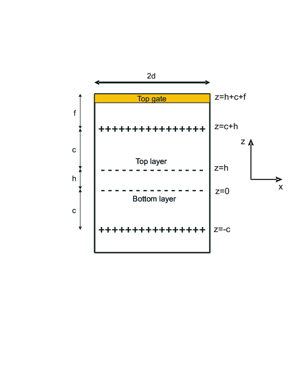
Figure 1: The cross-section of the bilayer geometry. Sample is capped by a gate from top in order to change the electron density of the top-layer. Top (bottom) 2DES lies below (above) the top (bottom) layer donors at a distance, $c$. Electron layers are separated from each other by a dielectric spacer having thickness, $h$.

One obtains the total electrostatic potential of an electron on the line $(x,z)$ due to a line-charge at $(x_{0},z_{0})$ fromSiddiki and Gerhardts (2003)

$$V(x,z)=V_{bg}(x,z)+V_{H}(x,z),$$ (1)

and

$$V_{H}(x,z)=\frac{2e^{2}}{\bar{\kappa}}\int_{x_{l}}^{x_{r}}dx_{0}K(x,x_{0},z,z_{0})n_{\rm el}(x_{0},z_{0}),$$ (2)

where $-e$ is the charge of an electron, $\bar{\kappa}$ an average background dielectric constant, and the kernel $K(x,x_{0},z,z_{0})$ solves Poisson’s equation under the relevant boundary conditions given by

$$K(x,x_{0},z,z_{0})=-\frac{1}{2}\ln\!\left(\frac{\cos^{2}\frac{\pi}{4d}(x+x_{0})+\gamma^{2}}{\sin^{2}\frac{\pi}{4d}(x-x_{0})+\gamma^{2}}\right)$$ (3)

where the $z-$ dependence is given by $\gamma=\sinh(\pi|z-z_{0}|/4d)$, due to a missprint a factor $1/2$ was missing in our previous work, although the numerics included this factor. The confining (background) potential is obtained by inserting a constant number density ($n_{0}$) of the background charges into Eq. (2). It is assumed that the gate can be described by an induced charge distribution $n_{g}(x)$, residing on the plane $z_{g}$. Then, from Eq.(2) the gate potential can be written as

$$V_{g}(x,z)=\frac{2e^{2}}{\bar{\kappa}}\int_{-d}^{d}dx_{0}K(x,x_{0},z,z_{g})n_{\rm g}(x_{0}).$$ (4)

Figure 2: The gate potential profile (solid-line) at $z=h$, together with the generating positive charge distribution (dotted-line) against position. The additional charges residing on the gate lead to a stronger confining potential in the top layer, resulting in a higher average electron density. The gate potential strength is taken to be $n_{g}^{0}/n_{0}=0.02$, where $E_{0}$ is the pinch-off energy. It is defined as $E_{0}=(2\pi e^{2}n_{0}d/\bar{\kappa})(\pi^{2}/8G)$ normalized with $G=0.915965594$, the Catalan’s constantGradshteyn and Ryzhik (1994) for $\gamma=0$. The donor density is $n_{0}=4\cdot 10^{11}cm^{-2}$. For other parameters see text.

In order to obtain a flat (gate) potential profile at the bulk we choose the induced charge distribution as

$$n_{g}(x)=n_{g}^{0}(1+\alpha(x/d)^{2}),$$ (5)

where $n_{g}^{0}$ determines the strength of the gate potential whereas $\alpha$ gives the slope of the induced charge distribution. In Fig. 2 the distribution of the positive charges and the resulting potential profile is shown for $\alpha=0.7$. One can add more electrons to the top layer by setting $n_{g}^{0}/n_{0}$ to a positive value, while keeping the depletion length $d-b$ fixed at zero temperature and for vanishing magnetic field. With such treatment of the gate, the average electron densities are changed while the depletion length is kept constant. Similarly the Hartree potential is calculated from Eq.(2) for the top layer as

$$V_{H}^{T}(x,z)=\frac{2e^{2}}{\bar{\kappa}}\int_{-d}^{d}\!dx_{0}K(x,x_{0},z,z_{0}=h)n^{T}_{\rm el}(x_{0})$$

and for the bottom layer

$$V_{H}^{B}(x,z)=\frac{2e^{2}}{\bar{\kappa}}\int_{-d}^{d}\!dx_{0}K(x,x_{0},z,z_{0}=0)n^{B}_{\rm el}(x_{0}).$$

Then Eq.(1) can be rewritten as

$$V(x,z)=-V^{T}_{bg}(x,z)-V^{B}_{bg}(x,z)-V_{g}(x,z)$$

$$+V_{H}^{T}(x,z)+V_{H}^{B}(x,z).$$ (6)

In the next step the electron densities are calculated within the TFA:

$$n^{T,B}_{el}(x)=\int dED(E)f([E+V(x,z_{T,B})-\mu^{*}_{T,B}]/k_{B}T),$$ (7)

with $D(E)$ the Landau density of states (DOS), $f(E)=1/[\exp(E/k_{B}T)+1]$ the Fermi function, $\mu^{*}_{T,B}$ is the chemical potential (being constant in the equilibrium state) and $z_{T,B}$ the position of top and bottom layer, respectively. We will use the Landau DOS described by

$$D(E)=\frac{1}{\pi l^{2}}\sum_{n=0}^{\infty}{\delta(E-E_{n})},$$ (8)

as default, unless other definitions are given. In our numerical calculations, we start with zero temperature and magnetic field and initially obtain the confining potential created by its own donors for each layer.

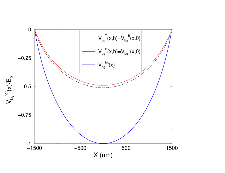
Figure 3: Total background potential created by the top and bottom layer donors (thick solid-line). The potential contributions to the bottom 2DES $(z=0)$ come from top donor layer ($V_{bg}^{T}(x,0)$, thin solid line) and from bottom donor layer ($V_{bg}^{B}(x,0)$, dashed line). Numerical calculations are performed for GaAs heterostructure with the parameters $h=15$nm and $c=60nm$. The numbers of donors are fixed to $4\times 10^{11}$cm^-2 per layer, for a sample width $2d\sim 3\mu$nm, with an average pinch-off energy $E_{0}$.

Then, we obtain the electron densities and the Hartree potentials of both layers just as in the case of a single layerSiddiki and Gerhardts (2003). Knowing the electron distribution of the top (bottom) layer via Eqs.(7) and (2) we calculate the potential acting on the bottom (top) layer similar to the single layer case. So that the total electrostatic potential of an electron at the top layer is

$$V^{T}(x)=V_{ext}(x,h)+V^{B}_{H}(x,h)+V^{T}_{H}(x,h),$$ (9)

where the total fixed external potential acting on the layers is $V_{ext}(x,z)=V^{tot}_{bg}(x,z)+V_{g}(x,z)$ and we denote the total background potential by $V^{tot}_{bg}(x,z)=V^{T}_{bg}(x,z)+V^{B}_{bg}(x,z)$ (see Fig.3). Note that the first two terms in Eq. (9), are considered to be external and the last term is the intra-layer Hartree potential. Similarly for the bottom layer the total electrostatic potential is

$$V^{B}(x)=V_{ext}(x,0)+V^{T}_{H}(x,0)+V^{B}_{H}(x,0).$$ (10)

In each iteration step an accurate numerical convergency is achieved for a single layer, then the Hartree potential is added to the other layers external potential. Intra-layer self-consistencies are obtained by Newton-Raphson iteration and inter-layer self-consistency is obtained by direct iteration. One can then use this solution as an initial value and obtain the density and screened potential for finite magnetic field and temperature. We scale energies by the average pinch-off energy $E^{*}_{0}=(E^{T}_{0}+E^{B}_{0})/2=E_{0}$, since we always assume symmetric donor distribution, e.g. $\Omega_{c}=\hbar\omega_{c}/E_{0}$ (and set the gate voltage to be zero, thus no extra charges reside on the top gate). The lengths are scaled by the screening length $a_{0}$ ($=a^{*}_{B}/2$) expressed in terms of effective Bohr radius, $a^{*}_{B}=\bar{\kappa}\hbar^{2}/(me^{2})$. The electron density and the electrostatic potential can be calculated self-consistently by the above scheme within the TFA.

III Screening results

In this section we present our results calculated within the self-consistent scheme, starting by discussing the zero temperature, zero magnetic field limit and then compare the obtained density profiles with the finite temperature and field profiles. The aim of this investigation is to clarify the effect of the quantizing perpendicular magnetic field, which introduces local charge imbalances due to formation of the incompressible strips. We have already seen that the electron density distribution is highly sensitive to the applied external magnetic and electric fields. Therefore even very small changes in these external parameters affect the density and potential profiles drastically.

It is well knownSiddiki and Gerhardts (2003) that the formation of the compressible and incompressible strips results in an inhomogeneous density distribution that deviates from the zero field profile. This deviation creates a local charge imbalance generating a potential fluctuation. We describe this fluctuation by,

$$\Delta V(x)=[V(x,0,0)-V(x,T,B)]/\Omega_{2},$$ (11)

where the self-consistent potentials are calculated at zero and finite magnetic field and temperature, respectively (see Fig.4b). Here after $\Omega_{2}$ ($=\hbar\omega_{c}/E_{0}=0.328\times 10^{-2}$) represents the dimensionless cyclotron energy at average filling factor two, since we always consider situations, where average filling factor is around two. We start our analysis by discussing the effect of the local charge deviation from its equilibrium distribution at $T=0\,,B=0$. Figure  4a depicts the electron densities calculated within the SCTFPA for vanishing and finite magnetic field and temperature, where we used $300$ mesh points to span a single layer. The typical parameters used in the calculations are: $d=1570$nm, $c=60$nm, $h=15$nm, $f=100$nm, $n_{0}=4\times 10^{11}$cm^-2 and for unbiased gate $\bar{n}^{T}_{el}=\bar{n}^{B}_{el}=3.31\times 10^{11}$cm^-2 which result in a Fermi energy ($E_{F}$) $\sim 14$meV. A positive (with respect to the electrons) potential bias is applied to the top gate [for details check Eq.(5) and related text] so that more electrons are populated to the top layer resulting in a density mismatch. The curves for finite field and temperature show a considerable deviation from the curves for zero field and temperature in the intervals ($200$nm$<|x|<1000$nm), where one observes incompressible strips at the top layer. In the inset we concentrate on this interval. In Fig. 4a we compare the $T=0,B=0$ density curves to the $T\neq 0,B\neq 0$ ones. In the interval $-600$nm$<x\lesssim-300$nm there are less electrons at the top layer due to the formation of an incompressible strip. This yields a less repulsive inter-layer Coulomb interaction. So that more electrons are populated locally at the bottom layer. Similar arguments hold for the left-hand side of the incompressible strip ($-800$nm$\lesssim x<-600$nm) but now the potential becomes more repulsive thus more electrons are depleted from the bottom layer locally. The corresponding potential variations are shown in Fig.4b, the peak like behavior near the edges results from temperature difference, whereas the structure observed at the top layer is due to the formation of the incompressible strip in the same layer. Since the bottom layer is completely compressible the potential variation does not show any non-monotonous feature and the fluctuation is perfectly screened. A relatively large variation is seen within the depletion regions. The reason for this is that, at finite temperature the density profiles leak out at the edges. At very strong magnetic fields ($\nu(0)<2$) only the lowest Landau level is partially occupied, i.e. high DOS, thus the density profiles for vanishing and for very strong magnetic field should look very similar. However, for intermediate $B$ there is a difference due to the quantizing magnetic field, that creates dipolar (incompressible) strips at the top layer, which have an influence on the bottom layer via the strong Coulomb interaction. Therefore, it is essential to examine the formation of the incompressible strips at strong magnetic fields. This is done by manipulating the sheet electron densities by applying a finite gate bias. The gate controls the existence and positions of the incompressible strips indirectly, so that one can examine the screening effects of the incompressible strips considering the electron density distributions. In the later sections, potential fluctuations created by these local charge imbalances, i.e. the incompressible strips, will be connected to the magneto-transport quantities, where we explicitly show the impact of the incompressible strips on the Hall resistances.

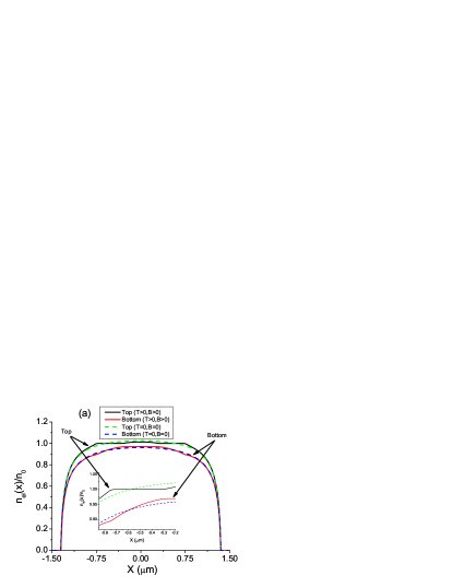
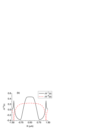
Figure 4: [a] Electron densities for a finite magnetic field (such that, $\bar{\nu}^{tot}_{av}=1.6$) and at default temperature ($kT/E_{0}=5\times 10^{-5}$ or $kT/E_{F}\sim 0.01$), for top and bottom (thin solid-line) layers. Also for vanishing field and temperature (dotted lines). [b] The resulting potential variation due to the formation of the incompressible strips, where the superscripts refers to top (T) and bottom (B). The depletion length is set to be $150$nm and the density mismatch is governed by applying a finite gate potential $V_{0}/E_{0}^{*}=0.02$, resulting in $\bar{n}_{el}^{T}=3.42\times 10^{11}$cm^-2 and $\bar{n}_{el}^{B}=3.18\times 10^{11}$cm^-2. The inset shows the region where an incompressible strip exists at the top layer.

III.1 Intra-layer distance, temperature and density mismatch

It is well known that the mutual Coulomb interaction is a strong long-range interaction. Thus, a change in the charge distribution, compared to the equilibrium distribution (at $T=0\,,B=0$), produces a considerable effect on the observable quantities even at large distances. In the previous section it is shown that such a local charge imbalance, connected with a potential fluctuation, is created due to formation of the incompressible strips. Here we investigate the density distributions of the layers by applying a positive gate voltage, hence populating the top 2DES and vary the intra-layer distance and temperature. The average total filling factor, $\bar{\nu}^{tot}_{av}=(\nu^{T}+\nu^{B})/2$, is kept constant and the evolution of the incompressible strip at the top layer, and its effect to the bottom layer, is examined. In Fig. 5 we show the local filling factors of both layers versus position, where the top layer (upper set of curves) has an incompressible strip in the interval $-850$nm$<x<-600$nm for different inter-layer distances. The influence of the incompressible strip in the top layer on the electron distribution of the bottom layer disappears rapidly although the intra-layer distance is changed rather smoothly. This is due to exponential decay of the amplitude of the Coulomb potential in the $z-$ direction, i.e. $V(q,z)\sim V_{q}\exp{-q|z|}$. The effective confining potential (ECP) experienced by each layer, of course, depends strongly on the inter-layer distance, hence for each $h$ value the number of electrons at each layer changes. This is depicted at the inset of Fig.5, there we concentrate to the center filling factor center. We observe that by increasing $h$($=30,60$ and $120$nm) the number of electrons at the center decreases (at fixed magnetic field) and the ECP becomes less confining thus a flatter density distribution is observed. Interestingly, for the largest separation ($h=200$nm) the bottom layer becomes widely incompressible at the bulk, hence semi-transparent, and the electrons of the top layer start to see the donors of the bottom layer. This specific configuration leads accumulation of the top layer electrons to the bulk and is a clear indication of non-linear screening, due to incompressible strips, in such a bilayer system. This fact emphasizes that even small a change at $h$ has a strong influence on the electron density profile. The exponential decay of the Coulomb interaction in the growth direction essentially determines whether the two 2DESs are strongly coupled or not, depending on the formation of the incompressible strips, i.e. screening. In the relevant experiments the distance between the two layers is fixed during the growth process. Hence we proceed our investigation by fixing $h=15$nm and vary the electron temperature. For such a separation the system is known to be electronically uncoupled and can be described by two electrochemical potentials.

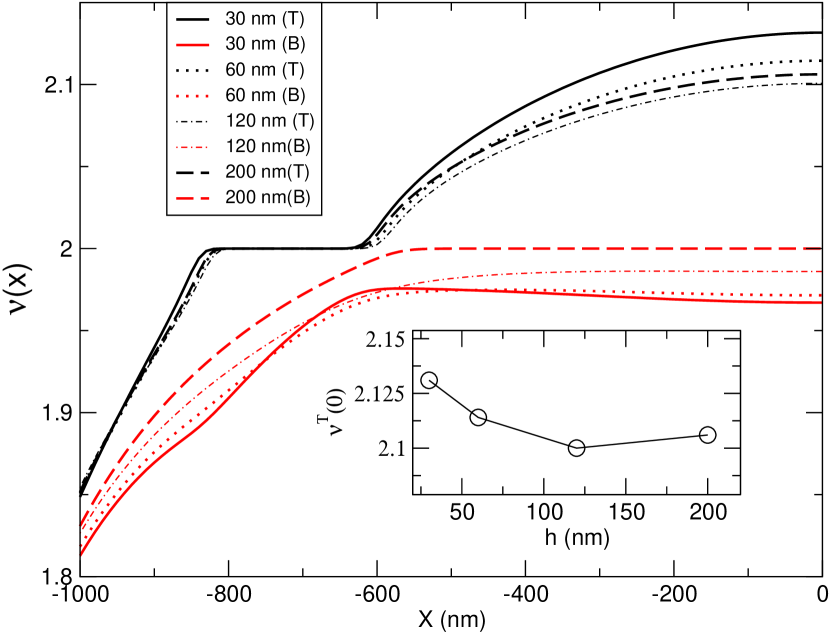
Figure 5: Local filling factors versus position at a finite magnetic field and for $h=30,60,120$ and $200$ nm, at default temperature. The top layer (upper set) exhibits an incompressible strip and whereas bottom layer (lower set) is compressible all over the electron channel, except $h=200$nm. The inset depicts the center filling factor of the top layer for four $h$ values.

In Fig. 6 the temperature dependence of the incompressible strip residing in the top layer and the compressible region at the bottom layer is shown. At single layer geometries it is well knownLier and Gerhardts (1994); Oh and Gerhardts (1997) that the quantizing effect of the magnetic field becomes inefficient, if the thermal energy of the system becomes larger than few percents of the cyclotron energy. Here we also observe a similar behavior for the bilayer system where the incompressible strip at the top layer and, moreover, the local charge imbalance seen at the bottom layer disappears while increasing the dimensionless temperature $t(=kT/E_{F})$ from 0.01 to 0.08. This fact shows that the local inhomogeneity at the bottom layer density distribution is only due to the dipolar strip at the top layer and is very sensitive to the temperature and exists for $t<0.04$.

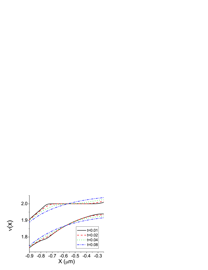
Figure 6: Density profiles across the incompressible strip at the top layer as a function of temperature. For a fixed density mismatch, $\bar{n}_{el}^{B}/\bar{n}_{el}^{T}=0.93$, at $\bar{\nu}^{tot}_{av}=1.6$ with $h=15$nm.

Relevant to the experiments considered, density mismatch is another tunable parameter, like the temperature. For this purpose now we fix the temperature and intra-layer distance and vary the potential of the top gate essentially by changing the number of induced positive charges. Figure 7 presents position dependent filling factors for such a positively charged gate, simulating different density mismatches by applying a gate bias voltage $V_{0}$. For a slight mismatch one does not observe a prominent change, except more electrons are accumulated at the center of the top layer. Due to the stronger Coulomb repulsion the bulk of the bottom layer is more depopulated and shows a flatter profile ( see Fig.7a). In Fig.7b, this feature is more pronounced at a higher gate bias and, in turn, the bottom layer is forced to be incompressible at the bulk, leading the effective external potential to be more confining for the top layer. The outer edge regions of incompressible strips residing at the top layer suppress the electrons beneath, at the bottom layer. Increasing the density mismatch in favor of the top layer, in Fig.7c and d, it is observed that more electrons start to accumulate at the bulk of the top layer and small density fluctuations can be seen at the bottom layer, however, we do not see any prominent change at the density profiles since the bottom layer can screen perfectly. We close our short discussion by noting that, even a small amount of density mismatch can lead to a drastic change in the density profiles. Moreover this change is enhanced by the existence of the incompressible strip, which results from the non linear screening in the presence of external magnetic field. This high sensitivity to the external electric field (here the gate) is clearly seen, if the potential profiles are considered. We shall emphasize, that a wide incompressible strip formed at the bulk of one of the layers does not necessarily imply that this layer becomes completely transparent to its donors, since the electrons residing in the incompressible strip create an electric field which can still partially cancel the electric field generated by its donors.

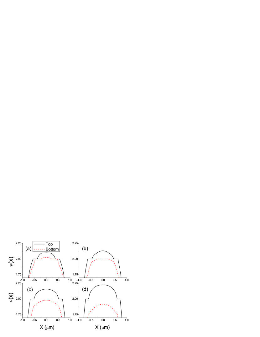
Figure 7: The top layer is populated by applying a finite gate potential $V_{0}/E_{0}^{*}$ [a] 0.01, [b] 0.02, [c] 0.03, [d] 0.05 corresponding to density mismatches of $\bar{n}_{el}^{B}/\bar{n}_{el}^{T}=0.96,0.93,0.89,0.84$, respectively. Given at default temperature, with the depletion length, $b/d=0.9$ and $\bar{\nu}_{av}^{tot}=1.67$.

III.2 Potential fluctuations

In this section we examine the effects of the incompressible strips in one layer on the external potential profile of the other layer by comparing what we call ”interacting” and ”non-interacting” systems. In both cases we start with the self-consistent calculation of the density and potential profiles at $T=0$, $B=0$. Then we focus on one layer, bottom or top, which we call the ”active” layer while the other layer is called the ”passive” one. Now we keep the $T=0$, $B=0$ density and Hartree potential profile of the passive layer fixed and calculate in the corresponding, $B-$ independent external potential of the active layer its density and potential profile self-consistently at finite $T$ and $B$. This yields the total potential $V_{N}(x,z)$ of the non-interacting system. It takes into account the $B-$ dependent intra-layer screening properties in the active layer, but not the $B-$ dependent changes of the intra-layer screening in the passive layer and of the inter-layer screening. Finally we drop the restriction on the passive layer and calculate density and potential profiles for both layers at finite $T$ and $B$ fully self-consistently. This yields the total potential $V_{I}(x,z)$ of the interacting system.
The potential variation (at finite temperature and magnetic field, indexed by $F$ as a subscript)

$$\Delta_{F}V(x)=[V_{I}(x,z)-V_{N}(x,z)]/\Omega_{2},$$ (12)

taken at the $z-$ value of the active layer, describes the $B-$ dependent change of the interaction of the active with the passive layer. It is suitable for studying the effect of the incompressible strips in the passive layer on the effective potential in the active layer. Fig. 8 shows potential variation and filling factors across the sample at four different magnetic field values where the superscript $T(B)$ indicates that the top (bottom) layer is the active layer. In Fig. 8a the magnetic field strength is chosen such that both layers are compressible, i.e. the center filling factors of both layers are slightly below two. The potential variation shows a characteristic behavior as the layers are both compressible all over the sample, the screening is nearly perfect and we do not observe any significant potential fluctuation. If one decreases the magnetic field strength and obtains a wide incompressible strip in the bulk of the top layer (Fig. 8b), a large potential variation is observed at this layer. This is nothing but the charge quadrupole at the center, treated by Ref.[Chklovskii et al., 1993] for a single layer geometry. The variation drastically increases and becomes almost $\sim\%30\Omega_{2}$. Meanwhile, the variation of the bottom layer does not show any significant change. The explanation of these observations is twofold; first as an incompressible strip is formed at the top layer, the finite field density profile strongly deviates from the zero field profile, which essentially creates a huge local (within the incompressible strip) external potential fluctuation to the bottom layer. Second, the bottom layer is completely compressible, so that this large potential fluctuation can be screened by redistribution of the bottom layer electrons, resulting in a density deviation from the zero $B$ profile. Note that as a consequence of the self-consistency the deviation is spread all over the bottom layer, which also generates an external potential fluctuation to the top layer. Here, as we examine how the top layer responds to this external potential fluctuation, we remind the reader that there are two different regions with different screening properties: (i) The compressible regions ($0.5\mu$m$<|x|<1.5\mu$m interval in Fig.8b) show similar features to the bottom layer and the external potential fluctuation is well screened, (ii) The incompressible region ($0\mu$m$<|x|<0.5\mu$m interval in Fig.8b) at the bulk can poorly screen the fluctuation and one observes that $\Delta_{F}V(x)$ can be large as half the Fermi energy.

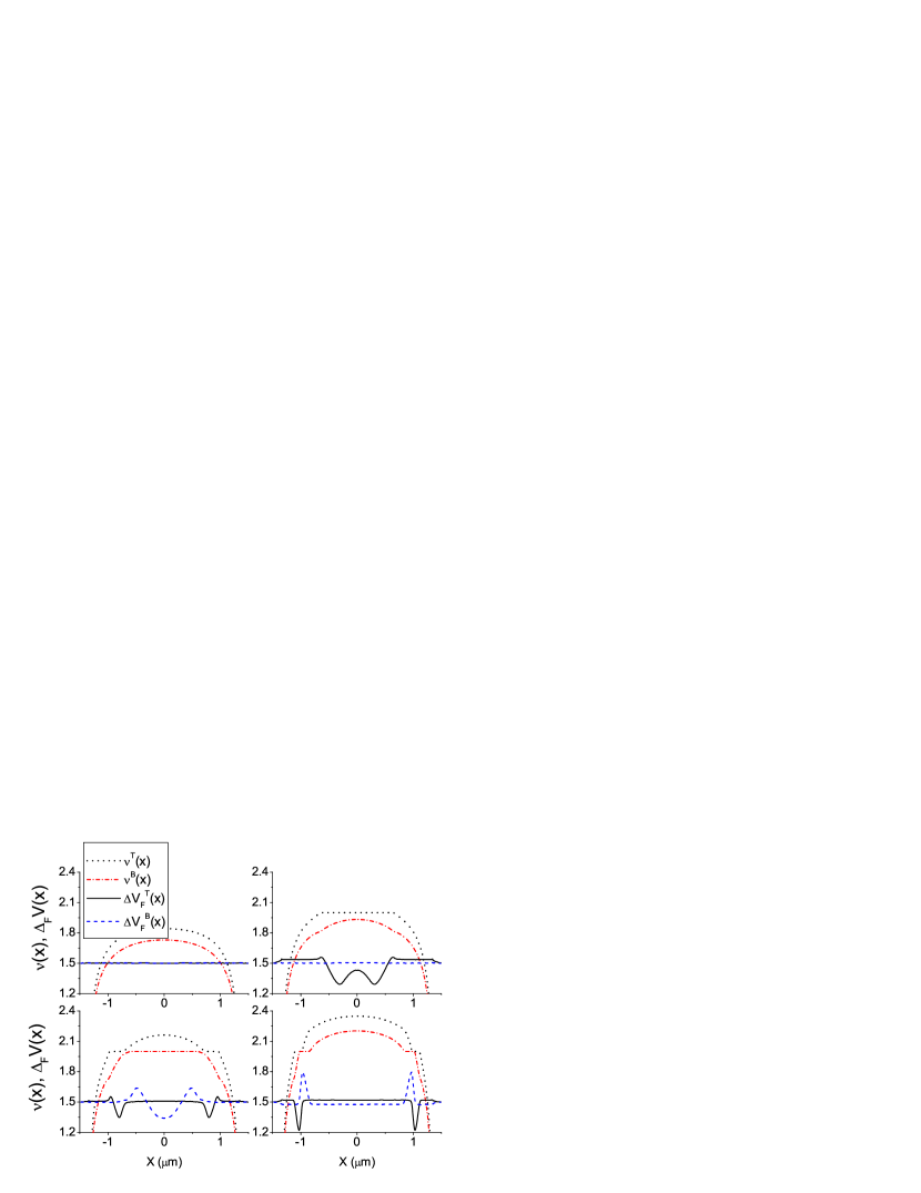
Figure 8: Position dependent filling factors and magnetic field induced potential variations, for $\bar{\nu}_{av}^{tot}$ [a] 1.44 [b] 1.59 [c] 1.69 [d] 1.84. For clarity all the potential variations are shifted by an amount of 1.5. The gate potential is set to $V_{0}/E_{0}^{*}=0.02$, for fixed depletion and at default temperature.

In Fig. 8c, the magnetic field strength is slightly decreased in order to obtain a wide incompressible strip at the bottom layer, meanwhile the wide incompressible strip of the top layer splits into two ribbons which are shifted towards the edges. For this $B$ value, one observes both the quadrupole (for the bottom layer) and the dipole (at the top layer) moments. Figure  8d shows the case, where two well developed incompressible strips are present at both of the layers and the potential fluctuations, created by the charge dipoles, are confined to these regions. Different than the previous case we only observe one side of the dipole moment, since the other half is screened by the other layer. We should emphasize that the variation amplitude depends on the width of the incompressible strip which generates the fluctuation, since the charge imbalance becomes larger if the incompressible strip is wide. The finding is simply that the potential fluctuations in a layer exist only within incompressible regions and are screened in compressible ones.

III.3 Modulated donor distribution

It is rather a common technique, to add an external (harmonic) modulation potential to the confinement potential in order to study the peculiar low-temperature screening properties of a 2DES, which has been done for a single layer geometry Wulf et al. (1988); Siddiki and Gerhardts (2002, 2003). Although a double layer geometry is a very promising system, even a qualitative investigation of such a modulation is still missing in the literature. In this section we provide a simple model to discuss the effect of this modulation on screening and compare our results, qualitatively, with the single layer ones.

A harmonic density modulation is added to the background charge distribution in order to obtain a potential modulation. Here we should also note that such a modulation will be used to simulate the long-range fluctuations of the confining potential in the following sectionsSiddiki and Gerhardts (submitted to Int. J. Mod. Phys. B). It is assumed that the spatial distribution of the donors is given by

$$n_{m}(x)=n_{0}\big{(}1-\delta\cos(\lambda\pi(x/2d))\big{)}$$ (13)

where $\lambda$ is an odd integer preserving the boundary conditions and $\delta$ describes the strength of the modulation. In the following discussion we will fix the density mismatch, $\bar{n}_{el}^{B}/\bar{n}_{el}^{T}=0.77$, modulation period, $\lambda=11$, temperature, $t=0.01$, and the average filling factor, $\bar{\nu}_{av}^{tot}=1.34$, to calculate the electrostatic quantities. We see in Fig.9 that the top layer is in phase with the modulation, whereas the bottom layers phase is shifted by an amount of $\pi/2$, where the modulation strength is chosen to be one percent. For the given parameters both layers are compressible and screening is still linear (see Fig.10 region (i)), i.e. the electrons can redistribute according to the applied external potential. A similar case for single layer geometries has been extensively studied in Ref.[Siddiki and Gerhardts, 2002, 2003] and the linear dielectric function is given by $\epsilon(q)=1+1/a_{0}q$ ($\sim 19$ for our parameters). This linear screening approximation breaks down when the amplitude of the screened potential becomes equal to the Fermi energy of the unmodulated systemWulf and Gerhardts (1988). From this we would expect that the breakdown amplitudes of the two layers should be directly proportional to the density mismatch. In order to test this and examine the non-linear screening regime we increase the strength of the modulation monotonously and look at the variation of the screened potential defined by,

$$var[V^{T,B}]=V^{T,B}(x=0)-V^{T,B}(x=0.3\mu m)]/\Omega_{2}.$$ (14)

Figure 10a presents this variation, for top (solid line) and bottom (dashed line) layers. In the regime denoted by (i) both layers are compressible and the density profile can be characterized similar to Fig.9. With increasing the modulation amplitude first the top layer enters to the non-linear screening regime, since incompressible strips are formed (see Fig.10b). This is pronounced as a jump in the variation an saturates at $\delta\sim 0.05$ (regime (ii)), meanwhile the bottom layer is still compressible, (i.e in the linear regime) and compensates (screens) the potential fluctuation generated [cf. discussion related to Fig.8b]. From the saturation point we can easily predict the similar point of the bottom layer to be $\delta\sim 0.07$. Actually we see that regime (iii) of Fig.10a starts at the expected value, where incompressible strips are present at both layers showing a characteristic distribution similar to Fig.8c. Here screening becomes linear again, but now with $\epsilon(q)=1+(D_{T}/D_{0})/(a_{0}q)$, where $D_{T}$ is the thermodynamic DOS in a Landau Level, which can be estimated by $D_{T}/D_{0}\sim\hbar\omega_{c}/(4k_{B}T)$. For $\delta>0.15$ the bottom layer is split to five narrower channels (see Fig.10d) and the linear screening is broken around $\delta\sim 0.16$. From the analytical expressions given in Ref.[Siddiki and Gerhardts, 2002] one can estimate the breakdown amplitude as

$$\delta_{bd}\sim\frac{2E_{F}^{B}.\epsilon(q)}{E_{0}}\sim 0.16,$$ (15)

which indeed is in very good agreement with the obtained numerical result. The small difference is due to the higher temperature and the decay of mutual Coulomb interaction in growth direction, likewise the difference at the slope of the plateaus. We also observe that the plateaus occur at the integer multiples of the individual filling factors, similar to the single layer system. Since we start with a situation where the average filling factors of the both layers are below two we see only one plateau, as discussed for the single layer geometries the number of the plateaus depend on the average filling factor without modulation. Finally we would like to note that the linear screening will break down for the top layer for $\delta\sim 0.2$ which can seen easily from Eq.15.

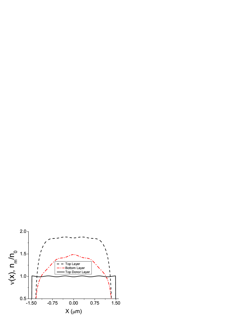
Figure 9: Spatial distribution of the donors (solid line), together with the local filling factors of top (dashes) and bottom (dashed-dots) layers at default temperature.

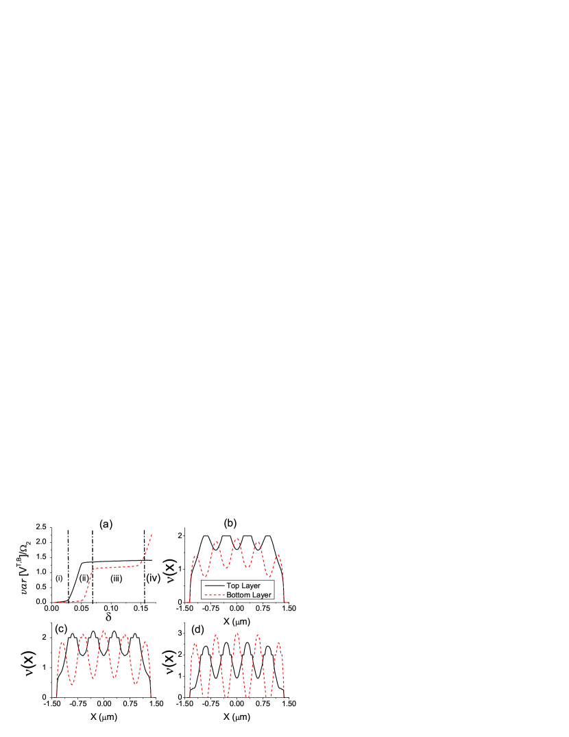
Figure 10: [a] The variation of the screened potential versus the modulation amplitude, together with the typical electron densities corresponding to different screening regimes [b] ii, $\delta=0.026$, [c] iii, $\delta=0.073$ and [d] iv, $\delta=0.157$. For top (solid lines) and bottom (dashed lines) layers.

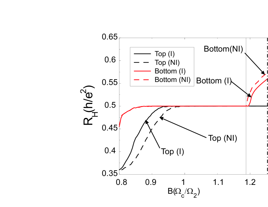
Figure 11: Comparison of the interacting (solid-lines) and non-interacting (dashed-lines) Hall resistance curves for fixed electron densities at default temperature. The Hall resistance curve is shifted for the top layer as the potential fluctuation created by the bottom layers incompressible strip.

The potential fluctuations and the donor modulation discussed above plays an important role when one considers a fixed external current flowing through both of the layers. These fluctuations are generated by local charge imbalances, with respect to zero field density distributions, and can be observed in the interval where the other layer has an incompressible strip as they are poorly screened.

IV The Hall resistance curves

In this section we investigate the effects of potential fluctuations on the Hall resistances using the findings of SGSiddiki and Gerhardts (2004a) within the linear response regime. In their work it was concluded that the (long-range) potential fluctuations can widen, stabilize and shift the quantized Hall (QH) plateaus as they affect the position and the existence of the incompressible stripsSiddiki and Gerhardts (submitted to Int. J. Mod. Phys. B). In addition to the long-range fluctuations, in this section we also include the potential fluctuations generated by the local charge imbalances. Here we use the general expressions derived in Ref.[Siddiki and Gerhardts, 2004a], for a given electron density and fixed current, to calculate the Hall and longitudinal resistances, of the bilayer system. We also note that the averaging procedure of the conductivities is carried over a length scale ($\lambda_{av}$), which is comparable with the Fermi wavelength and, in particular is set to be $40$nm in our calculations. We apply these results to two cases considered in Sec. III.2, namely the interacting and non-interacting systems. We remind that, in the case of non-interacting system, the active layer does not have information about the density inhomogeneities caused by the incompressible strips of the passive layer. Hence comparing the resistance curves of these two cases essentially gives a method to extract the effect of the incompressible strips on the other layer.

In order to investigate the relation between the incompressible strips of the passive layer and the magneto-transport coefficients of the active layer qualitatively, we calculate the Hall resistances for a magnetic field interval, where QH plateaus are observed for both layers around filling factor two. In Fig. 11 we show the Hall resistances (in units of the von Klitzing constant) vs. magnetic field for interacting (solid-lines) and non-interacting (dashed lines) systems. We start the discussion with the high-magnetic field regime ($\Omega_{c}/\Omega_{2}>1.27$, i.e right side of the vertical dotted line), which essentially corresponds to a density distribution similar to that shown in Fig. 8a. As there are no incompressible strips within both layers, no noticeable potential fluctuations are created due to local charge imbalance, therefore the Hall resistances of both layers are the same for interacting and non-interacting cases. If we examine the QH regime of the top layer (the regime between vertical dash-dotted line and dotted line in Fig.11), it is seen that at least one incompressible strip is formed (cf. Fig. 8b), creating a potential fluctuation to the bottom layer. Meanwhile, the bottom layer is still compressible all over the sample, so the fluctuation can be screened nearly perfect, leading to a new distribution of the electrons and a small change in the $R_{H}$ curves, due rearrangement of the local conductivities. The situation is fairly different, in the interval $1.18<\Omega_{c}/\Omega_{2}<1.25$ (the region between thin vertical solid-line and dashed-dotted line), where incompressible strips are formed at both of the layers (density distributions corresponding to Fig. 8c and Fig. 8d). In this regime, where both layers produce fluctuations due to local charge imbalance and this fluctuation can not be screened perfectly everywhere, which should result in a difference in the Hall resistance curves. This is observed for the bottom layer at the high-magnetic field edge, since the perturbation slightly shifts the maximum magnetic field value of the QH plateau. In this regime the quantized value of the Hall resistance of the top layer does not change, since it only depends on the presence of the incompressible strip. In the $1<\Omega_{c}/\Omega_{2}<1.18$ interval of Fig.11 there exists two stable incompressible strips in both layers surrounded by compressible regions, thus both layers are in the QH plateau. Here we should note that, although the potential fluctuations are created by the incompressible strips and are not screened perfectly, this perturbation changes only the positions or the widths of the incompressible strips, but not the value of the $R_{H}$ within the plateau regime. Eventually it depends on the amplitude of the perturbation, i.e. if the amplitude is large enough to destroy the incompressible strips one does not observe the quantized value for $R_{H}$. The change in $R_{H}$ can be observed for the top layer at somewhat smaller values of the magnetic field strength ($0.8\lesssim\Omega_{c}/\Omega_{2}\lesssim 1.0$) since the perturbation enlarges the plateau. In fact the fluctuation widens the incompressible strips, with respect to the non-interacting case and creates incompressible strips larger than the averaging length, $\lambda_{av}$. Finally one ends with a wider plateau. The difference in the Hall resistance curves between the interacting and non-interacting systems, tends to disappear as the incompressible strips become narrower and move towards the edges by decreasing the magnetic field. This is consistent with the previous observation, that the amplitude of the fluctuation depends on the width of the incompressible region.

In summary four magnetic field intervals are observed: (i) both layers are compressible and there exists no difference for the $R_{H}$ curves, calculated for the interacting and non-interacting case, (ii) top layer, at least, has an incompressible strip and creates a fluctuation, which shifts for the bottom layer the edge of the Hall plateau to higher magnetic field values, (iii) both layers show incompressible regions, the perturbation generated by the bottom layer widens the incompressible strips of the top layer, leading to a wider plateau, (iv) the incompressible strips of both layers become narrower and move towards the edges and the fluctuation becomes inefficient, hence the difference is smeared out. It is useful to mention that the interacting system is an equilibrium solution, in the sense that the electrons of both layers rearrange their distribution until a full convergence is obtained (within a numerical accuracy), for a given external potential profile.

V Comparison to the experiments

Here we report on the magneto-transport hysteresis observed in the bilayer systems measured at the Max-Planck Institut-Stuttgart by S. KrausSiddiki et al. (2006). In the experiments discussed here, the magneto-resistances are measured as a function of the applied perpendicular magnetic field. The sweep direction dependence is investigated for matched and mismatch densities. Similar findings have already been presented in the literatureTutuc et al. (2003); Pan et al. (2004), however, have been discussed in a different theoretical content.

The samples are GaAs/AlGaAs double quantum well structures grown by molecular beam epitaxy (MBE). Separate Ohmic contacts to the two layers are realized by a selective depletion techniqueEisenstein et al. (1990). A technique developed by Rubel et al.[Rubel et al., 1998] was used to fabricate backgates. The metal gate on top of the sample acts as frontgate. The samples were processed into $80\mu$m wide and $880\mu$m long Hall bars. The high mobility samples are grown at the Walter-Schottky Institut. They have as grown densities in the range $1.5-2.5\times 10^{11}$cm^-2 and mobility is 100 m²/Vs per layer. The barrier thickness is 12nm and the quantum wells are 15nm wide. The experiments were performed at low-temperatures (T 270mK) and the imposed current is always in the linear response regime (I$\sim 50$nA). Other details of the experimental setup and samples could be found in an upcoming publicationSiddiki et al. (2006).

We show the measured Hall resistances of the top layer (solid lines for up and dashed lines for down sweep) and the bottom layer (dotted lines for up and dashed-dotted lines for down sweep) as a function of magnetic field strength and direction in Fig.12. The data were taken at a sweep rate $0.01$T/min and the base temperature is always kept at $270$mK. Apparently it is seen that the resistances of the layers follow different traces depending on whether the sweep is in up or down direction, in certain $B$ field intervals. We see that the sweep direction has no effect on the resistances at high magnetic fields ($B>8$T), where we would not expectSiddiki and Gerhardts (2004a) to have any incompressible strips (see e.g. Fig8a). The first exiting feature is observed when the bottom layer is in the plateau regime and the top layer is approaching to its plateau regime ($6.5$T$<B<8.5$T). It is seen that the Hall resistance of the top layer follows two different traces depending on the sweeping direction, meanwhile the bottom layers resistance is insensitive and assumes the quantized value.

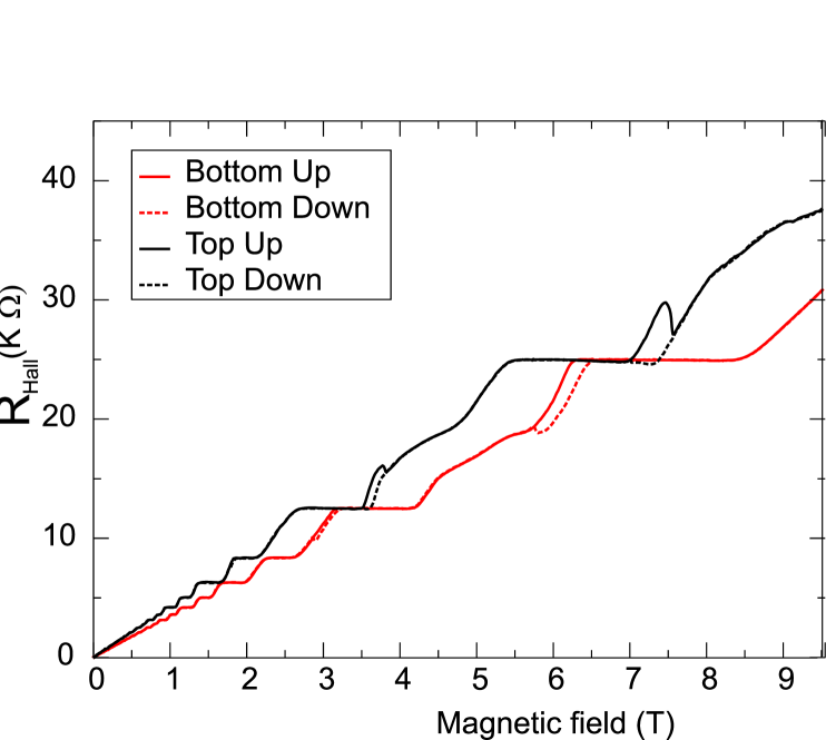
Figure 12: The Hall resistances as a function of magnetic field for a GaAs electron bilayer system with a barrier width 12nm, considering two sweep directions. Data is taken at a magnetic sweep rate $0.01$T/min. A strong hysteresis develops in $R_{H}$ when the other layer is in a plateau. No significant effect is observed at low field regime.

The plateau regime is extended up to $B\sim 7.25$T for down sweep and ends at $B=7$T for up sweep, meanwhile the bottom layer is also in the QH regime. It is easy to understand why the QH regime is wider for the down sweep considering the widths of the incompressible strips as follows: while coming form high magnetic field to low fields we first encounter with a wide incompressible region at the bottom layer (see for example Fig.8b, of course here bottom layer has a higher density) that generates a large potential fluctuation yielding a wide plateau. However, for the other sweep direction two narrow incompressible strips are observed first (Fig.8d), which creates relatively weak fluctuations, that have a negligible effect on the plateau width. For smaller values of the magnetic field, we observe at the top layer that up and down sweep curves follow the same trace and have the quantized value at $B=6.8$T. A similar hysteresis behavior is seen at the bottom layer resistance curves ($5.7$T$<B<6.5$T), now the top layer is in the plateau regime for both sweeping directions. The resistances at low magnetic field interval ($4$T$<B<7$T) do not show a prominent difference for two sweep directions. A less pronounced repetition of the hysteresis is observed at the $\nu=2$ plateau regimes, e.g. $3.4$T$<B<3.6$T and $2.9$T$<B<3.2$T. A common feature (also observed at different density mismatches) is that the hysteresis is seen at the active layer only if the passive layer is in the plateau regime. No hysteresis is observed if the QH regimes of the layers coincide (see discussion in Ref.[Siddiki et al., 2006]). We summarize the experimental observations as follows: the hysteresis is observed in the active layer only if the passive layer is in the plateau regime.

We should mentioned that the hysteresis effect is a non-equilibrium effect and ”interacting” system is an equilibrium solution, hence can not explain this effect directly. However, it is easy to attribute the widening of the top layer s plateau (for down sweep) to the potential fluctuations created by the bottom layer, as already shown for the ”interacting” case in Fig.11. In accord with our numerical results (previous section) obtained for the ”non-interacting” system, the measured quantities are independent of their history. We claim that the measured resistances are the analogues of the calculated resistances for the non-interacting system for the up sweep of the top layer, since the incompressible strips are narrow and the potential fluctuations are ineffective.

VI Summary

In this work we have studied the screening properties of an electron-electron bilayer system. The electrostatic part is solved numerically using a self-consistent screening theory by exploiting the slow variation of the confining potential. We compared the electron distributions for vanishing magnetic field and temperature with the finite ones, and observed that a local charge imbalance is created due to the formation of incompressible strips. These dipolar strips produce external potential fluctuations, as a function of applied magnetic field, to the other layer. We have investigated properties of this potential fluctuation by comparing the interacting and non-interacting systems for a few characteristic $B$ values and obtained the Hall resistances by a local scheme proposed in our recent workSiddiki and Gerhardts (2004a). We considered these fluctuations as a perturbation to the other layer and observed that they widen, stabilize and shift the plateaus as expected. In Sec.V we have report and attempted to obtain qualitative arguments for the hysteresis-like behavior by reconsidering the symmetry breaking of the sweep direction, based on the long relaxation times of the incompressible regions. This is done by considering the ”interacting” and ”non-interacting” schemes. Our results show that the Hall resistance curves follows different paths if both of the layers have incompressible strips within the sample. The amplitude of the deviation depends on the widths and the positions of the incompressible regions.