Realistic network growth using only local information:
From random to scale-free and beyond

Abstract

We introduce a simple one-parameter network growth algorithm which is able to reproduce a wide variety of realistic network structures without having to invoke any global information about node degrees such as preferential-attachment probabilities. Scale-free networks arise at the transition point between quasi-random and quasi-ordered networks. We provide a detailed formalism which accurately describes the entire network range, including this critical point. Our formalism is built around a statistical description of the inter-node linkages, as opposed to the single-node degrees, and can be applied to any real-world network – in particular, those where node-node degree correlations might be important.

Networks – in particular, large networks with many nodes and links – are attracting increasing attention from researchers in the fields of physics and biology through to sociology, informatics and medicine random ; Newman ; Barabasi ; pakming ; Holme ; Leary ; Krapivsky ; Saramaki ; Evans ; Batagelj98 ; Callaway ; Vazquez . Many social and informational networks, including the World Wide Web, exhibit scale-free behaviour while others lie closer to fully-random or fully-ordered random ; Newman . Growth mechanisms have been proposed for a wide variety of such networks – however, many of these growth mechanisms require some form of global knowledge of the vertex (i.e. node) degree. In particular, the famous preferential-attachment model of Barabási and Albert Barabasi requires knowledge of each node’s degree in order to evaluate the corresponding attachment probability. Holme and Kim Holme and Leary et al Leary have subsequently considered a modification of this preferential rule by ranking existing nodes according to degree, and associating corresponding probabilities of connection with the new node accordingly. Their approach led to over- and under-skewed distributions for the node degree, as compared to the power-law distribution characteristic of scale-free networks. However in both the original and modified preferential-attachment algorithms, information is required about the degree – and hence preferential-attachment probability – of every node in the network, prior to adding a new node or link.

Although preferential attachment models can yield similar distributions to real-world systems, this requirement that the next node or link ‘knows’ about the degree of every node in a large network, makes the mechanism microscopically unrealistic for many real-world networks. In particular, most biological and social networks are too large for such information to be accessible. Motivated by this shortcoming, the present paper discusses a simple, one-parameter algorithm which can reproduce under-skewed, over-skewed and scale-free (i.e. power-law) networks without global knowledge of the node degrees – see Figs. 1 and 2. It therefore provides an alternative, and arguably more realistic, microscopic mechanism for a wide range of biological and social networks, whose growth had previously been explained using the Barabási-Albert preferential–attachment model Barabasi . As a by-product of our analysis, we also provide a new formalism to describe general network growth dynamics including node-node linkage correlations. When applied to our growth algorithm, this ‘link-space’ formalism allows us to identify the transition point at which over-skewed node-degree distributions switch to under-skewed distributions. It is at this transition point, and only at this point, that we find scale-free networks emerge. Similar notions of transitive linking have been studied elsewhere Krapivsky – in particular, Saramaki and Kaski Saramaki and Evans Evans have recently presented some fascinating results using random-walkers to decide node attachment in a network-growth algorithm. However, these analyses were all mean-field in nature and hence were not able to accurately describe the node-node linkage correlations which can be a crucial feature of real-world networks, and are a crucial feature of the one-parameter networks discussed here.

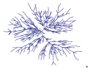
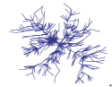
Figure 1: (Color Online) Networks generated by our one-parameter, local information growth algorithm with $a=1$ (left), $a=0.2$ (center), $a=0$ (right).

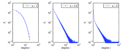
Figure 2: (Color Online) Degree distributions for the networks in Fig. 1, grown to 100,000 nodes and ensemble-averaged over 100 networks per $a$-value. Initial seed comprised two nodes and one link.

We first introduce our general formalism. We then use it to discuss various existing growth algorithms and our one-parameter growth algorithm, together on the same footing. For a growing network in which one node and undirected link are added at timestep $t$, we can write the master equation for $X_{i}$ (the number of nodes of degree $i$) in terms of the probabilities $\{\Theta_{j}\}$ for attaching to a node of degree $j$:

$$X_{i}\mid_{t+1}=X_{i}\mid_{t}+\Theta_{i-1}\mid_{t}-\Theta_{i}\mid_{t},\ \ \ i>1\ \ .$$ (1)

The second term describes the probability of the new node attaching to an existing node of degree $i-1$ thereby making it a degree $i$ node. The third term on the right hand side describes the new node attaching to a node of degree $i$, thereby decreasing $X_{i}$. For $i=1$, the second term is unity as a new node of degree one is added to the existing network each timestep. If we assume steady-state growth, then $X_{i}=c_{i}t$ and hence the fraction of nodes of degree $i$ is constant ($\frac{dX_{i}}{dt}=c_{i}$). To facilitate the comparison with later expressions, we write the solution in the following form:

$$c_{i}=\frac{\Theta_{i-1}}{1+\frac{\Theta_{i}}{c_{i}}}$$ (2)

The notation ‘$\mid_{t}$’ has been dropped to indicate steady-state. So far we have said nothing about the attachment mechanism, and have made the easily geneneralizable restriction that only one node and undirected link is being added per timestep. We now follow a similar analysis, but retain the node-node linkage correlations that are inherent in many real-world systems Callaway ; Krapivsky . Consider any link in a general network – we can describe it by the degrees of the two nodes that it connects. Hence we can construct a matrix $\mathbf{L}$ such that the element $L_{i,j}$ describes the number of links from nodes of degree $i$ to nodes of degree $j$. For undirected networks, the summation over all elements $L_{i,j}$ is equal to twice the total number of links in the network. This matrix represents a surface describing the first-order correlations between the node degrees – we refer to this as the link space.

In order to write the master equations for the evolution of the network in this link space, we must first understand the impact of adding a new link. The probability of selecting any node of degree $i-1$ is given by the attachment kernel $\Theta_{i-1}$. Suppose an $i-1$ node is selected – the fraction of these that are connected to nodes of degree $j$, is $\frac{L_{i-1,j}\mid_{t}}{(i-1)X_{i-1}\mid_{t}}$. The term describing the increase in links from nodes of degree $i$ to nodes of degree $j$, through the attachment of the new node to a node of degree $i-1$, is given by:

$$\frac{\Theta_{i-1}\mid_{t}L_{i-1,j}\mid_{t}}{X_{i-1}\mid_{t}}\ \ \ .$$ (3)

Since each link has two ends, the value $L_{i,j}$ can increase by connection to an $(i-1)$-degree node which is in turn connected to a $j$-degree node, or by connection to an $(j-1)$-degree node which is in turn connected to an $i$-degree node.

We now make a similar steady-state assumption to the ‘node space’ example above, and obtain David :

$$l_{i,j} = \frac{\frac{\Theta_{i-1}}{c_{i-1}}l_{i-1,j}~{}+~{}\frac{\Theta_{j-1}}{c_{j-1}}l_{i,j-1}}{1~{}+\frac{\Theta_{i}}{c_{i}}~{}+~{}\frac{\Theta_{j}}{c_{j}}},\ \ \ ~{}~{}~{}i,j>1;$$

$$l_{1,j} = \frac{\frac{\Theta_{j-1}}{c_{j-1}}l_{1,j-1}~{}+~{}\Theta_{j-1}}{1~{}+\frac{\Theta_{1}}{c_{1}}~{}+~{}\frac{\Theta_{j}}{c_{j}}},\ \ \ ~{}~{}~{}~{}~{}~{}~{}~{}j>1;$$ (4)

where $l_{i,j}$ denotes the fraction of links that connect an $i$-degree node to a $j$-degree node. It turns out that $l_{1,1}$ is zero for all the growth algorithms discussed in this paper, since the networks that they generate comprise a single component. The notation $\mid_{t}$ has been dropped as before, to indicate the steady state. The fraction of $i$-degree nodes is:

$$c_{i}=\frac{\sum_{k}l_{i,k}}{i}\ \ ,\ \ X_{i}=\frac{\sum_{k}L_{i,k}}{i}\ .$$ (5)

Hence the degree distribution is retrievable from the link-space matrix. To illustrate use of the formalism, consider first a random-attachment model in which the existing node to which the new node is to be connected, is chosen randomly. The attachment probability is $\Theta_{i}~{}=~{}c_{i}$. Substituting into Eq. 2, we obtain the recurrence relation $c_{i+1}=\frac{c_{i}}{2}$ which yields the familiar $2^{-i}$ distribution of node degree. Substituting into the link-space master equation (Eq. 4) yields the recurrence relations:

$$l_{i,j} = \frac{l_{i-1,j}+l_{i,j-1}}{3},\ \ \ \ ~{}~{}~{}~{}i,j~{}>1;$$

$$l_{1,j} = \frac{c_{j-1}+l_{1,j-1}}{3},\ \ \ \ ~{}~{}~{}~{}j>1;$$

$$l_{1,1} = 0\ \ \ .$$ (6)

The exact solution for $l_{i,j}$ is

$$\sum_{\alpha=2}^{j}\frac{{}^{(i-1+j-\alpha)}C_{(j-\alpha)}}{3^{(i+j-\alpha)}2^{(\alpha-1)}}+\sum_{\alpha=2}^{i}\frac{{}^{(i-1+j-\alpha)}C_{(i-\alpha)}}{3^{(i+j-\alpha)}2^{(\alpha-1)}},\ \ \ \ ~{}~{}~{}i,j>1;$$

$$\sum_{k=1}^{j-1}\frac{1}{3^{k}2^{j-k}},\ \ \ \ ~{}~{}~{}i=1,j>1,$$ (7)

where $C$ is the conventional combinatorial ‘choose’ function. The surface generated is shown in Fig. 3.

In the Barabási-Albert preferential attachment algorithm Barabasi , the attachment probability is proportional to the degree of the node in the existing network:

$$\Theta_{i}\mid_{t}=\frac{iX_{i}}{2(N-1)}$$ (8)

which in the steady-state limit of large $N$ (i.e. many nodes) can be well approximated by $\Theta_{i}\approx\frac{ic_{i}}{2}$. Substituting this expression into Eq. 2 yields the familiar recurrence relation

$$c_{i}=\frac{(i-1)~{}c_{i-1}}{2}-\frac{i~{}c_{i}}{2}=\frac{i-1}{i+2}c_{i-1}$$ (9)

whose solution is:

$$c_{i} = \frac{4}{i(i+1)(i+2)}\ \ \ .$$ (10)

Using the same substitution, the link-space master equations yield the recurrence relations:

$$l_{i,j} = \frac{(i-1)l_{i-1,j}~{}+~{}(j-1)l_{i,j-1}}{2+i+j},\ \ \ ~{}~{}~{}i,j>1;$$

$$l_{1,j} = \frac{(j-1)c_{j-1}~{}+~{}(j-1)l_{1,j-1}}{3+j},\ \ \ ~{}~{}~{}j>1\ \ .$$ (11)

The exact solution for $l_{i,j}$ is obtained by algebraic manipulation of the link-space matrix using the previously derived degree distribution, and is given by David :

$$\begin{array}[]{l}l_{i,j}=\frac{4(j-1)!(i-1)!}{(j+i+2)!}\Big{\{}G(i+1)+2G(i)-3G(i-1)\\ +\frac{1}{2}\sum_{\alpha=1}^{i}(\alpha-1)(\alpha+6)\left[G(i-\alpha)-G(i-\alpha-1)\right]\Big{\}};\\ G(x)~{}=~{}\left\{\begin{array}[]{l r}\frac{(j+x-1)!}{x!(j-1)!}&\textrm{for $x\geq 0$}\\ 0&\textrm{for $x<0$}\ .\end{array}\right.\end{array}$$

The first two rows of this matrix, have the form:

$$l_{1,j} = \frac{2(6+j)(j-1)}{j(j+1)(j+2)(j+3)};\ \ \ \$$

$$l_{2,j} = \frac{2j(j-1)(j+10)+48}{3j(j+1)(j+2)(j+3)(j+4)}\ .$$ (12)

The above equations for $l_{i,j}$, even when invoked to low order in the iteration scheme, can accurately reproduce the Barabási-Albert preferential attachment network. The corresponding surface is shown in Fig. 3.

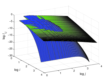
Figure 3: (Color Online) Representation of the link-space matrix with elements $l_{i,j}$, in logarithmic coordinates. The values shown are the steady-state solutions for the random attachment (curved surface) and preferential attachment (flatter surface) algorithms. The value $l_{1,1}$ is zero for networks consisting of a single component.

We now turn to our one-parameter network growth model, which involves attaching a single node at each timestep without prior knowledge of the existing network structure. The algorithm goes as follows: i) Pick a node $\kappa$ within the existing network at random. ii) With probability $a$ make a link to that node. Otherwise iii) pick any of the neighbours of $\kappa$ at random, and link to that node. Hence this algorithm resembles an object or ‘agent’ making a short random-walk. Figure 1 shows examples of the resulting networks, with Fig. 2 showing the corresponding degree distributions. Interestingly, $a=0$ yields a graph that is dominated by hubs and spokes (i.e. extreme over-skewed) footnote1 while $a=1$ yields the random-attachment graph. Intermediate values of $a$ yield networks which are neither too ordered nor too disordered. For $a\sim 0.2$, the algorithm generates networks whose degree-distribution closely resembles Barabási-Albert preferential-attachment networks (see Figs. 1, 2 and 4).

We now develop master equations for the evolution of this one-parameter network generated with only local information. We first establish the attachment probability kernel $\Theta_{i}$ for this algorithm, which in turn requires properly resolving the one-step random walk. The link-space formalism provides us with an expression for the probability $P^{\prime}_{i}$ associated with performing a random walk of length one and arriving at a node of degree $i$. Note that this is different to arriving at a specific node of degree $i$ after a one-step walk, since here we consider the possibility of arriving at any of the nodes which happen to have degree $i$ at time $t$ David :

$$P^{\prime}_{i} = \frac{X_{1}\mid_{t}L_{1,i}\mid_{t}}{N_{t}X_{1}\mid_{t}}+\frac{X_{2}\mid_{t}L_{2,i}\mid_{t}}{2N_{t}X_{2}\mid_{t}}+\frac{X_{3}\mid_{t}L_{3,i}\mid_{t}}{3N_{t}X_{3}\mid_{t}}+\ldots$$ (13)

$$= \frac{1}{N_{t}}\sum_{k}\frac{L_{k,i}\mid_{t}}{k}$$

This can also be written David as $P^{\prime}_{i}=\frac{iX_{i}\mid_{t}}{N_{t}}\langle\frac{1}{k}\rangle_{i}$ where the average is performed over the neighbours of nodes with degree $i$. Note that this quantity does not replicate preferential attachment, in contrast to what is commonly thought  Saramaki ; Vazquez . Defining $\beta_{i}$ as

$$\beta_{i}\equiv\frac{1}{i~{}c_{i}}\langle\frac{1}{k}\rangle_{i}=\frac{\sum_{k}\frac{L_{i,k}}{k}}{\sum_{k}L_{i,k}}=\frac{\sum_{k}\frac{l_{i,k}}{k}}{\sum_{k}l_{i,k}}\ ,$$ (14)

yields

$$\Theta_{i}=ac_{i}~{}+~{}(1-a)\beta_{i}ic_{i}$$ (15)

Substituting Eq. 15 into Eq. 2, we obtain the following for the steady-state node degree:

$$c_{i}=\frac{c_{i-1}\big{(}a+(1-a)\beta_{i-1}(i-1)\big{)}}{1+a+(1-a)\beta_{i}i}\ \ .$$ (16)

Substituting into Eq. 4 yields the following recurrence relations:

$$l_{i,j}=\frac{l_{i-1,j}\big{(}a+(1-a)\beta_{i-1}(i-1)\big{)}+l_{i,j-1}\big{(}a+(1-a)\beta_{j-1}(j-1)\big{)}}{1+2a+(1-a)(i\beta_{i}+j\beta_{j})}$$

$$l_{1,j}=\frac{l_{1,j-1}\big{(}a+(1-a)\beta_{j-1}(j-1)\big{)}+c_{j-1}\big{(}a+(1-a)\beta_{j-1}(j-1)\big{)}}{1+2a+(1-a)(\beta_{1}+j\beta_{j})}\ .$$

The non-linear terms resulting from $\beta$ imply that an explicit closed expression for $l_{i,j}$ is difficult. We leave this as a future challenge – but we stress that our formalism can be implemented in its non-stationary form numerically (i.e. iteratively) with very good efficiency David , as demonstrated by the degree distributions in Fig. 4.

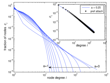
Figure 4: (Color Online) Degree distributions generated using the link-space analysis of our one-step algorithm. Inset: results for $a=0.25$ reproduce the same distribution as for the Barabási-Albert Barabasi preferential-attachment algorithm.

Our numerical results suggests that for $a\sim 0.2$, the degree distribution approaches scale-free. We now use the above formalism to deduce the critical value $a_{c}$ at which the node-degree distribution goes from over-skewed to under-skewed, and hence the value of $a$ at which a scale-free distribution arises. At $a_{c}$, we know that the attachment kernels for both our and the Barabási-Albert model should be equal. Hence from Eq. 8 and Eq. 15, we have

$$\frac{i}{2}=a_{c}~{}+~{}(1-a_{c})\beta_{i}i$$ (17)

which for large $i$ yields $a_{c}=1-\frac{1}{2\beta_{i}}$. We could proceed to use the exact solution of the link-space equations for the preferential-attachment algorithm, in order to infer $\beta_{i}$ in the high $i$ limit. However, since $\beta_{i}$ can be expanded in terms of $l_{i,j}$ as shown in Eq. 14, and $l_{i,j}$ decays very rapidly as $i,j$ become large, we can obtain a good approximation by only using the first two terms of Eq. 12. This gives $\beta\sim 0.66$. Substituting into Eq. 17 then yields the critical value at which scale-free networks exist as $a_{c}=0.25$, in excellent agreement with the results shown in the inset plot of Fig. 4.

In conclusion, we have presented a simple, one-parameter algorithm for generating networks whose properties span from the exponential degree distribution of random attachment, through to an ordered ‘hub and spoke’ situation (Fig. 1). A scale-free network turns out to be a special case, lying at a transition point in between the two limits. The growth algorithm utilizes only one simple parameter $a$, and requires no global information concerning node degree. As a by-product of the analysis of this model, we have managed to develop a new type of link-space formalism which can account for the node-node linkage correlations in real-world networks. Indeed, as will be shown elsewhere, the link-space formalism can be used to describe an even wider variety of networks than those emerging from the present growth model.

References

- (1) S.N. Dorogovtsev and J.F.F. Mendes, Evolution of Networks (Oxford University Press, Oxford, 2003)
- (2) M. Newman, A.L. Barabasi, D.J. Watts, The Structure and Dynamics of Networks (Princeton University Press, Princeton, 2006)
- (3) A.L. Barabási and R. Albert, Science 286, 509 (1999)
- (4) H. Y. Lee, H. Y. Chan, P. M. Hui, cond-mat/0402009
- (5) P. Holme and B.J. Kim, Phys. Rev. E 65, 026107 (2002)
- (6) C.C. Leary et al, physics/0602152 (2006)
- (7) P.L. Krapivsky and S. Redner, Phys. Rev. E 63, 066123 (2001)
- (8) J.P. Saramaki and K. Kaski, cond-mat/0404088 (2004)
- (9) T.S. Evans and J.P. Saramaki, Phys. Rev. E 72, 26138 (2005)
- (10) V. Batagelj and A. Mrvar, Connections 21, 47 (1998)
- (11) D.S. Callaway et al, Phys. Rev. E 64, 041902 (2001)
- (12) A. Vázquez, Phys. Rev. E 67, 056104 (2003)
- (13) For mathematical details and derivations, see www.physics.ox.ac.uk/users/smithdmd/linkspace.pdf
- (14) Suppose we seed the algorithm with an existing hub and spoke graph, and use . The probability that a new node will be linked to the hub tends to unity as the network grows. More generally, the distribution of vertex degrees will approach that of a hub and spoke network as the network grows. This type of network can be considered the most ordered in that the mean free path is minimized (i.e. it tends to two)