Coulomb Drag and Spin Coulomb Drag in the presence of Spin-orbit Coupling

Abstract

Employing diagrammatic perturbation theory, we calculate the (charge) Coulomb drag resistivity $\rho_{D}$ and spin Coulomb drag resistivity $\rho_{\uparrow\downarrow}$ in the presence of Rashba spin-orbit coupling. Analytical expressions for $\rho_{D}$ and $\rho_{\uparrow\downarrow}$ are derived, and it is found that spin-orbit interaction produces a small enhancement to $\rho_{D}$ and $\rho_{\uparrow\downarrow}$ in the ballistic regime while $\rho_{D}$ is unchanged in the diffusive regime. This enhancement in the ballistic regime is attributed to the enhancement of the nonlinear susceptibility (i.e. current produced through the rectification of the thermal electric potential fluctuations in the passive layer) while the lack of enhancement in the diffusive regime is due to the suppression by disorder.

I Introduction

Recent years have seen the emergence of a strong interest in exploiting the manipulation of the spin degrees of freedom in solid state systems that could lead to enhanced performance in electronic devices; this field of spin electronics, or simply spintronics RMP , has evolved into an exciting subject in condensed matter physics. Among the myriad of spintronics proposals, gate-controlled Rashba spin-orbit (SO) coupling has attracted tremendous attention as it offers the possibility of all-electrical spin manipulation without the presence of a magnetic field. One such experimentally realizable heterostructure is a double quantum well gate-modulated with Rashba spin-orbit coupling. In this paper, we study theoretically the effect of spin-orbit coupling on the Coulomb drag properties of 2D bilayer systems. As is well known, there exists Coulomb coupling between the barrier-separated two-dimensional electron gas (2DEG) layers induced by the momentum exchanges of the Coulomb-scattered electrons residing in individual layers. This phenomenon of Coulomb drag (in the absence of spin-orbit coupling), first observed experimentally by Gramila et al. Gramila between two 2DEG layers, has continued to be a subject of thorough investigation DragReview ; with a theoretical description developed in Refs. MacDonald ; Jauho2 ; Oreg ; Jauho . The physical mechanism at work in Coulomb drag can be understood as follows: The application of a current through one layer (the active layer) causes thermal fluctuations in the electron density, which are transferred across the barrier to the other layer (the passive layer) due to momentum exchanges by electron-electron scattering. In the passive layer, the variations in electrical potential associated with the thermal fluctuations in electron density then produce a current due to second-order rectification effect, quantified by the nonlinear susceptibility which is the response function connecting the random potential fluctuations and the induced electrical current. The drag resistivity $\rho_{D}$, which is defined as $\rho_{D}=E_{\mathrm{passive}}/j_{\mathrm{active}}$ — the ratio of the electric field strength developed in the open-circuited passive layer to the current density in the active layer, is a useful experimental measure of the Coulomb drag phenomenon.

Although the subject of Coulomb drag has existed since the first experiment more than a decade ago, it remains a very vibrant research topic today: recent experimental HoleD1 and theoretical HoleD2 studies have revealed that bilayer hole drag in the low density regime is a factor of $\sim 10^{2}-10^{3}$ larger than the corresponding electron drag. Moreover, other more recent experiments HoleD3 ; HoleD5 have shown that the low-density bilayer hole drag in the presence of an in-plane magnetic field (i.e. magnetodrag) has a qualitative dependence on the applied magnetic field unexpectedly similar to that of the single-layer magnetoresistivity, and this surprising observation has been accounted for theoretically by properly considering the suppression of screening by carrier spin polarization within the framework of the standard Fermi-liquid theory HoleD4 . In light of these recent developments, a very interesting question is whether spin-orbit coupling (which is effectively a momentum-dependent in-plane magnetic field) would change the qualitative behaviour of the drag resistivity. To our knowledge, the effect of spin-orbit coupling on Coulomb drag has not yet been investigated, and this problem is highly relevant in view of the current growing interest in viable semiconductor spintronic systems and especially potential device applications employing gate-controlled spin-orbit coupling.

The bilayer Coulomb drag provides direct quantitative information about carrier interaction effects since the drag voltage in the passive layer arises entirely due to the carrier-carrier scattering between the layers. The study of bilayer Coulomb drag properties in the presence of spin-orbit coupling effects therefore introduces a method of investigating the interplay between spin-orbit coupling and interaction effects. Since both spin-orbit coupling and interaction can be tuned by applying external electric and magnetic fields respectively, and also by changing the 2D density, the possibility exists for a detailed understanding of the interplay between spin-orbit coupling and many-body interaction effects through bilayer drag studies. This is a main motivation for our theoretical work.

On the other hand, it has also been proposed that there exists an analogous effect, called the spin Coulomb drag Vignale1 , in which spin-up and spin-down electrons within one single device structure (three- or two-dimensional) play the roles of the electrons in each individual layers in the charge Coulomb drag problem, and now it is the Coulomb scattering between the spin-up and spin-down carriers that causes the frictional force, damping the relative motion of the two spin components. Therefore, unlike ordinary charge current, the flow of opposite spin carriers (i.e. spin current) is a non-conserved quantity even without spin-orbit coupling and tends to be suppressed because of this drag effect. In the same spirit as $\rho_{D}$, one gains a measure of the spin drag by defining $\rho_{\uparrow\downarrow}=E_{\uparrow}/j_{\downarrow}$, the spin drag resistivity given by the ratio of the gradient of the electrochemical potential of spin-up carriers to the current density of the spin-down carriers, with the current of the spin-up carriers held zero. This effect has been confirmed in a recent experimental paper by Weber et al. Weber where it was found that the suppression of the measured spin diffusion coefficient relative to the charge diffusion coefficient could be explained by a correction factor $1/(1+|\rho_{\uparrow\downarrow}|/\rho)$ coming from the theoretical spin drag prediction. We note that while the Coulomb drag refers to a bilayer system, spin drag refers to a single 2D layer (or a single 3D system) with the up and down components of the spin playing the role of the “active” and “passive” carrier components.

The purpose of the present paper is to investigate the effect of spin-orbit interaction on the drag phenomenon in semiconductor structures including the usual (charge) Coulomb drag and the spin Coulomb drag. We follow Refs. Oreg ; Jauho and apply diagrammatic perturbation theory to calculate the Coulomb drag resistivity $\rho_{D}$ and spin Coulomb drag resistivity $\rho_{\uparrow\downarrow}$ in the presence of Rashba SO coupling. We find that for clean samples the Coulomb drag resistivity and the spin drag resistivity are enhanced by a correction factor $\Delta\rho_{D,\uparrow\downarrow}/\rho_{D,\uparrow\downarrow}\sim\mathcal{O}(\gamma^{2})$ in the presence of SO coupling ($\gamma$ is the dimensionless spin-orbit coupling strength), whereas for dirty samples the spin-orbit coupling correction to the Coulomb drag is essentially completely suppressed by disorder.

Our paper is organized as follows: we begin in section II with the problem of Coulomb drag, where after recapitulating a set of useful formulas related to Rashba SO coupling and Coulomb drag we proceed to evaluate in both the ballistic limit (subsection A) and the diffusive limit (subsection B) the nonlinear susceptibility, the central quantity in the problem. These results are then used in subsection C to calculate the Coulomb drag resistivity in the presence of Rashba SO coupling. With the aid of the formalism applied to the Coulomb drag, we turn in section III to the problem of spin Coulomb drag and calculate the spin drag resistivity in the ballistic regime. Finally conclusions are presented in section IV.

II Coulomb Drag

The electronic Hamiltonian in the presence of the Rashba SO coupling

$$H=\frac{p^{2}}{2m}+\alpha\left(\bm{\sigma}\times\bm{p}\right)\cdot\hat{\bm{z}},$$ (1)

has the following eigenstates

$$|\bm{p}\mu\rangle=\frac{1}{\sqrt{2}}\left[\begin{array}[]{c}1\\ \mu ie^{i\phi}\end{array}\right]|\bm{p}\rangle,$$ (4)

which is labelled by the quantum number $\mu=\pm 1$ called the chirality. The corresponding eigenenergy spectra follow as $\epsilon_{\bm{p}\pm}=p^{2}/2m\mp\alpha p$. We note that the transformation which diagonalizes the Hamiltonian Eq. (1) is a local transformation, dependent on the momentum $\bm{p}$ through $\mathrm{tan}\phi=p_{y}/p_{x}$:

$$U_{\bm{p}}=\frac{1}{\sqrt{2}}\left[\begin{array}[]{cc}1&1\\ ie^{i\phi}&-ie^{i\phi}\end{array}\right].$$ (7)

In the presence of Rashba SO coupling, the Fermi energy $\varepsilon_{F}=\hbar^{2}k_{F}^{2}/2m$ of the system is lowered in comparison to the case without SO coupling for the same number of electrons and there exists two branches of Fermi wavevectors $k_{F\pm}$ corresponding to the two chiralities. From $\epsilon_{\bm{k}}\mp\alpha\hbar k-\varepsilon_{F}=0$ we can express the two solutions $k_{\pm}$ in terms of $k_{F}$; on the other hand by particle conservation we have $n_{+}+n_{-}=k_{+}^{2}/4\pi+k_{-}^{2}/4\pi=k_{F}^{2}/2\pi$. Solving then yields the Fermi energy and Fermi wavevectors in the presence of Rashba SO coupling:

$$\varepsilon_{F} = \varepsilon_{F0}\left(1-2\gamma^{2}\right),$$ (8)

$$k_{F\pm} = k_{F0}\left(\pm\gamma+\sqrt{1-\gamma^{2}}\right),$$ (9)

where $\varepsilon_{F0}$ and $k_{F0}$ are the Fermi energy and Fermi wavevector without SO coupling, here we also define the dimensionless spin-orbit coupling strength $\gamma=\alpha/v_{F0}\ll 1$. The density of states $\nu$ at the Fermi level is readily found as

$$\nu_{\pm}=\nu\left(1\pm\frac{\gamma}{\sqrt{1-\gamma^{2}}}\right),$$ (10)

where $\nu=m/2\pi\hbar^{2}$ is the density of states per spin. In the following we proceed to evaluate the Coulomb drag resistivity of a double-layer 2DEG system with Rashba spin-orbit coupling. Using linear response theory, the drag resistivity is obtained from the diagrammatic expansions in Fig. 1 and is given by Oreg ; Jauho :

$$\rho_{\mathrm{D}} = \frac{\hbar}{16\pi k_{B}T\sigma_{1}\sigma_{2}}\sum_{\bm{q}}\int_{0}^{\infty}\frac{\mathrm{d}\omega}{\mathrm{sinh}^{2}\left(\hbar\omega/2k_{B}T\right)}$$ (11)

$$\Gamma_{1x}\left(q,\omega\right)\Gamma_{2x}\left(q,\omega\right)\left|U_{12}\left(q,\omega\right)\right|^{2}.$$

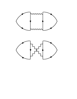
Figure 1: Diagrams contributing to the drag resistivity Eq. (11). For Coulomb drag (spin Coulomb drag), the wavy lines represent interlayer (intralayer) Coulomb potential; the vertices on the left and on the right denote charge current in layer 1 and layer 2 (spin-up current and spin-down current) respectively.

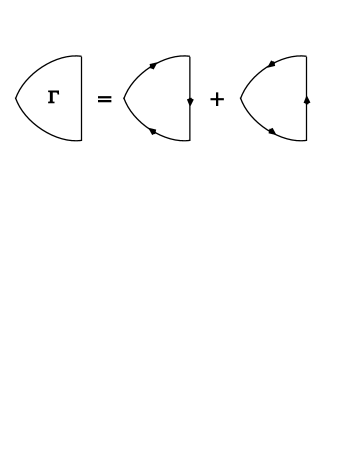
Figure 2: The three-point vertex representing the nonlinear susceptibility $\Gamma$. The vertex on the right side represent current vertex while the two vertices at the top and the bottom represent charge density vertices.

where $\sigma=2e^{2}\nu D$ is the Boltzmann conductivity of the individual layer ($D=\varepsilon_{F0}\tau/m$ is the diffusion constant), the subscripts ‘1’,‘2’ signify quantities in layer 1 and 2 respectively. $U_{12}$ is the screened interlayer potential which is obtained from solving the corresponding Dyson equation in the random phase approximation (RPA), $\bm{\Gamma}$ is the nonlinear susceptibility and is given from the three-point vertex diagrams in Fig. 2 as

$$\bm{\Gamma}(\bm{q},\omega)=\frac{1}{2\pi i}\int\mathrm{d}\varepsilon\left[n_{F}(\varepsilon+\omega)-n_{F}(\varepsilon)\right]\sum_{p}\mathrm{tr}$$

$$\;\left\{\left[G_{\varepsilon}^{A}(\bm{p}-\bm{q})-G_{\varepsilon}^{R}(\bm{p}-\bm{q})\right]G_{\varepsilon+\omega}^{A}(\bm{p})\bm{J}(\bm{p})G_{\varepsilon+\omega}^{R}(\bm{p})\right\}$$

$$+\left\{\bm{q},\omega\to-\bm{q},-\omega\right\},$$ (12)

where $G_{\varepsilon}^{R,A}(\bm{p})=(\varepsilon-H\pm i\hbar/2\tau)^{-1}$ denotes the retarded/advanced Green function, and $\mathrm{tr}$ the trace. Note that in the expression of the drag resistivity Eq. (11), because of the denomenator $\mathrm{sinh}^{2}(\hbar\omega/2k_{B}T)$, the dominant contribution of the $\varepsilon$ integral comes from the region $\hbar\omega\lesssim k_{B}T$, and therefore at low temperatures the dominant contribution to the drag resistivity comes from small values of $\omega$. In the following sections we evaluate Eq. (12) in respect to two regimes: ballistic regime ($\omega\tau>1$ or $ql>1$) and diffusive regime ($\omega\tau,ql\ll 1$), where $l=v_{F0}\tau$ is the mean free path.

II.1 Ballistic limit

In the ensuing discussions we express all Green functions and currents in the chiral basis, making use of the transformation Eq. (7). To this end we define the transformation $U_{+}=U_{\bm{p}}^{{\dagger}}U_{\bm{p}+\bm{q}}$ and $U_{-}=U_{+}^{{\dagger}}=U_{\bm{p}}^{{\dagger}}U_{\bm{p}-\bm{q}}$; explicitly,

$$U_{+}=\frac{1}{{2}}\left[\begin{array}[]{cc}1+\mathrm{e}^{i\theta}&1-\mathrm{e}^{i\theta}\\ 1-\mathrm{e}^{i\theta}&1+\mathrm{e}^{i\theta}\end{array}\right],$$ (15)

where $\theta=\phi_{\bm{p}+\bm{q}}-\phi_{\bm{p}}=\phi_{\bm{p}}-\phi_{\bm{p}-\bm{q}}$ is the scattering angle from momentum $\bm{p}$ to $\bm{p}+\bm{q}$ (or equivalently from momentum $\bm{p}-\bm{q}$ to $\bm{p}$). It will be useful to also note that $U_{+,-}^{{\dagger}}=U_{+,-}^{*}$ since $U_{+,-}$ is a symmetric matrix.

After a change of variable in $\varepsilon$ in the second term and a transformation into the chiral basis, Eq. (12) can be written as

$$\bm{\Gamma}(\bm{q},\omega) = \frac{1}{2\pi i}\int\mathrm{d}\varepsilon\left[n_{F}(\varepsilon+\omega)-n_{F}(\varepsilon)\right]\sum_{p}\mathrm{tr}\left\{U_{-}\left[\tilde{G}_{\varepsilon}^{A}(\bm{p}-\bm{q})-\tilde{G}_{\varepsilon}^{R}(\bm{p}-\bm{q})\right]U_{-}^{{\dagger}}\tilde{G}_{\varepsilon+\omega}^{A}(\bm{p})\tilde{\bm{J}}(\bm{p})\tilde{G}_{\varepsilon+\omega}^{R}(\bm{p})\right.$$ (16)

$$\left.-U_{+}\left[\tilde{G}_{\varepsilon+\omega}^{A}(\bm{p}+\bm{q})-\tilde{G}_{\varepsilon+\omega}^{R}(\bm{p}+\bm{q})\right]U_{+}^{{\dagger}}\tilde{G}_{\varepsilon}^{A}(\bm{p})\tilde{\bm{J}}(\bm{p})\tilde{G}_{\varepsilon}^{R}(\bm{p})\right\},$$

where the tilda represents quantities expressed in the chiral basis. In the ballistic limit, the charge current in the chiral basis is given by

$$\tilde{J}_{x} = \frac{\hbar k_{x}}{m}-\alpha\tilde{\sigma}_{y}$$ (19)

$$= \left[\begin{array}[]{cc}\hbar k_{x}/m-\alpha\mathrm{cos}\phi&i\alpha\mathrm{sin}\phi\\ -i\alpha\mathrm{sin}\phi&\hbar k_{x}/m+\alpha\mathrm{cos}\phi\end{array}\right].$$

In the following we will denote the matrix elements of $\tilde{J}_{x}$ as $\tilde{J}_{ij}$ for brevity. Here it will be useful to note that the off-diagonal elements are related by the hermiticity of $\tilde{\bm{J}}$ as $\tilde{J}_{12}=\tilde{J}_{21}^{*}=-\tilde{J}_{21}$.

Consider the energy integration of the first term in Eq. (16):

$$\int\mathrm{d}\varepsilon\left[n_{F}(\varepsilon+\omega)-n_{F}(\varepsilon)\right]\mathrm{tr}\left\{U_{-}\left[\tilde{G}_{\varepsilon}^{A}(\bm{p}-\bm{q})-\tilde{G}_{\varepsilon}^{R}(\bm{p}-\bm{q})\right]U_{-}^{{\dagger}}\tilde{G}_{\varepsilon+\omega}^{A}(\bm{p})\tilde{\bm{J}}(\bm{p})\tilde{G}_{\varepsilon+\omega}^{R}(\bm{p})\right\}$$ (20)

$$= i\frac{2\pi\tau}{\hbar}\left\{\tilde{J}_{11}\left[\left(1+\mathrm{cos}\theta\right)\mathrm{Im}\left\{\frac{n_{F}(\epsilon_{\bm{p-q}+})-n_{F}(\epsilon_{\bm{p}+})}{\omega+\epsilon_{\bm{p-q}+}-\epsilon_{\bm{p}+}+i0^{+}}\right\}+\left(1-\mathrm{cos}\theta\right)\mathrm{Im}\left\{\frac{n_{F}(\epsilon_{\bm{p-q}-})-n_{F}(\epsilon_{\bm{p}+})}{\omega+\epsilon_{\bm{p-q}-}-\epsilon_{\bm{p}+}+i0^{+}}\right\}\right]\right.$$

$$\;\;\;\;\;\;\;\;\,+\tilde{J}_{22}\left[\left(1+\mathrm{cos}\theta\right)\mathrm{Im}\left\{\frac{n_{F}(\epsilon_{\bm{p-q}-})-n_{F}(\epsilon_{\bm{p}-})}{\omega+\epsilon_{\bm{p-q}-}-\epsilon_{\bm{p}-}+i0^{+}}\right\}+\left(1+\mathrm{cos}\theta\right)\mathrm{Im}\left\{\frac{n_{F}(\epsilon_{\bm{p-q}+})-n_{F}(\epsilon_{\bm{p}-})}{\omega+\epsilon_{\bm{p-q}+}-\epsilon_{\bm{p}-}+i0^{+}}\right\}\right]$$

$$\left.\;\;\;\;\;\;\;\;+2\pi\tilde{J}_{12}\mathrm{sin}\theta\mathrm{Im}\left\{\frac{n_{F}(\epsilon_{\bm{p-q}+})-n_{F}(\epsilon_{\bm{p}+})}{\omega+\epsilon_{\bm{p-q}+}-\epsilon_{\bm{p}+}+i0^{+}}-\frac{n_{F}(\epsilon_{\bm{p-q}-})-n_{F}(\epsilon_{\bm{p}-})}{\omega+\epsilon_{\bm{p-q}-}-\epsilon_{\bm{p}-}+i0^{+}}\right\}\delta\left(\epsilon_{\bm{p}+}-\epsilon_{\bm{p}-}\right)\right\}.$$

We notice that the last term in Eq. (20) contains a delta function $\delta\left(\epsilon_{\bm{p}+}-\epsilon_{\bm{p}-}\right)=\delta\left(2\alpha p\right)$, which forces this term to vanish identically upon performing the momentum integration in Eq. (16), and hence, rather unexpectedly, the off-diagonal terms in the current Eq. (19) drop out and only the diagonal terms contribute to the nonlinear susceptibility. The same analysis above follows for the second term in Eq. (16), and the expression for the nonlinear susceptibility reduces to (with the notation $\tilde{J}_{++,--}=\tilde{J}_{11,22}$):

$${\Gamma}_{x}(\bm{q},\omega)=\frac{\tau}{\hbar}\sum_{\mu,\mu^{\prime}=\pm}\sum_{\bm{p}}\tilde{J}_{\mu\mu}(\bm{p})\left(1+\mu\mu^{\prime}\mathrm{cos}\theta\right)$$ (21)

$$\mathrm{Im}\left\{\frac{n_{F}(\epsilon_{\bm{p-q}\mu^{\prime}})-n_{F}(\epsilon_{\bm{p}\mu})}{\omega+\epsilon_{\bm{p-q}\mu^{\prime}}-\epsilon_{\bm{p}\mu}+i0^{+}}-\frac{n_{F}(\epsilon_{\bm{p}\mu^{\prime}})-n_{F}(\epsilon_{\bm{p+q}\mu})}{\omega+\epsilon_{\bm{p}\mu^{\prime}}-\epsilon_{\bm{p+q}\mu}+i0^{+}}\right\}.$$

Up to this point we have not yet made use of any simplifying assumptions and Eq. (21) for the ballistic case is general. Now, we evaluate Eq. (21) in the limit of low-energy $u\ll 1$ and long-wavelength $x\ll 1$, and we neglect the interband terms ($\mu\neq\mu^{\prime}$) as these are readily shown to be smaller than their intraband counterparts ($\mu=\mu^{\prime}$) by an order of $\mathcal{O}(q^{2}/k_{F0}^{2})$. At low temperatures $k_{B}T\ll\varepsilon_{F0}$, we expand the Fermi functions in $\varepsilon$ in Eq. (21) and keep up to $\mathcal{O}(\omega)$. The evaluation of a typical intraband term then goes as

$$\sum_{\bm{p}}\tilde{J}_{11}(\bm{p})\left(1+\mathrm{cos}\theta\right)\mathrm{Im}\left\{\frac{n_{F}(\epsilon_{\bm{p-q}+})-n_{F}(\epsilon_{\bm{p}+})}{\omega+\epsilon_{\bm{p-q}+}-\epsilon_{\bm{p}+}+i0^{+}}\right\}$$ (22)

$$= -\frac{2uk_{F0}}{\pi^{2}\hbar}\left(1+\frac{\gamma}{\sqrt{1-\gamma^{2}}}\right)\frac{u+x}{\sqrt{1-\gamma^{2}}},$$

where $u=\omega/v_{F0}q$ and $x=q/2k_{F0}$, $v_{F0}=\hbar k_{F0}/m$ is the Fermi velocity without spin-orbit coupling. Evaluating the rest of the intraband terms in the same manner, we find the nonlinear susceptibility Eq. (21) as

$${\Gamma}_{x}(q,\omega) = -\frac{4\nu Dq}{\varepsilon_{F0}}\frac{u}{\sqrt{1-\gamma^{2}}}$$ (23)

$$\simeq -\frac{4\nu Dq}{\varepsilon_{F0}}{u}\left(1+\frac{1}{2}\gamma^{2}\right).$$

Here we notice that the nonlinear susceptibility $\Gamma(q,\omega)$ is enhanced in the presence of SO coupling. In the ballistic limit, it should be emphasized that the nonlinear susceptibility without SO coupling is directly proportional to the imaginary part of the irreducible polarizability generally remark ; Jauho , independent of the low-energy long-wavelength assumption made on $u$ and $x$. Such a general statement is not true with SO coupling present, where it is readily seen that Eq. (21) is not, despite the similarity, explicitly proportional to the imaginary part of the irreducible polarizability in the presence of Rashba SO coupling saraga :

$$\Pi\left(q,\omega\right)=$$ (24)

$$-\frac{1}{2}\sum_{\mu,\mu^{\prime}=\pm}\sum_{\bm{p}}\left(1+\mu\mu^{\prime}\mathrm{cos}\theta\right)\frac{n_{F}(\epsilon_{\bm{p}\mu^{\prime}})-n_{F}(\epsilon_{\bm{p+q}\mu})}{\omega+\epsilon_{\bm{p}\mu^{\prime}}-\epsilon_{\bm{p+q}\mu}+i0^{+}}.$$

The reason here is that the current term $\tilde{J}_{11,22}(\bm{p+q})-\tilde{J}_{11,22}(\bm{p})$, with SO coupling (c.f. Eq. (19)), is no longer simply proportional to $q$ and so cannot be taken outside of the momentum integral. In the long-wavelength low-energy limit, however, proportionality is restored as can be seen by comparing with the following expression of the irreducible polarizability evaluated in the same limit:

$$\Pi\left(q,\omega\right)\simeq 2\nu\left(1+i\frac{u}{\sqrt{1-\gamma^{2}}}\right).$$ (25)

Therefore, in the ballistic regime, the enhancement of the nonlinear susceptibility Eq. (23) is physically attributable to the SO-induced enhancement of the intraband electron-electron scattering.

II.2 Diffusive limit

For low temperatures $k_{B}T\ll\varepsilon_{F0}$, we expand the Fermi functions in $\varepsilon$ in Eq. (12) and keep up to $\mathcal{O}(\omega)$. Transforming into the chiral basis, $\Gamma$ can then be expressed as

$$\bm{\Gamma}(\bm{q},\omega)=-\frac{\omega}{2\pi i}\sum_{p}\mathrm{tr}$$ (26)

$$\left\{U_{-}\left[\tilde{G}_{\varepsilon_{F}}^{A}(\bm{p}-\bm{q})-\tilde{G}_{\varepsilon_{F}}^{R}(\bm{p}-\bm{q})\right]U_{-}^{{\dagger}}\right.$$

$$\left.\;\;\tilde{G}_{\varepsilon_{F}+\omega}^{A}(\bm{p})\tilde{\bm{J}}(\bm{p})\tilde{G}_{\varepsilon_{F}+\omega}^{R}(\bm{p})\right\}+\left\{\bm{q},\omega\to-\bm{q},-\omega\right\}.$$

Since the spin-orbit coupling strength is assumed to be weak $\gamma\ll 1$, we retain terms up to the first nonvanishing order of $\mathcal{O}(\gamma^{2})$. In the diffusive limit $\omega\ll 1/\tau,q\ll 1/l$, we also expand Eq. (26) in terms of these parameters up to the first nonvanishing order, e.g. for the Green function we have

$$\tilde{G}_{\varepsilon_{F}}(\bm{p}\pm\bm{q})\simeq\tilde{G}_{\varepsilon_{F}}(\bm{p})\pm\bm{q}\cdot\hat{\bm{p}}\left(\frac{p}{m}-\alpha\sigma_{z}\right)\left[\tilde{G}_{\varepsilon_{F}}(\bm{p})\right]^{2}.$$ (27)

For the charge current vertex in the Rashba model, taking account of the diffuson pole correction exactly cancels the spin-dependent term in the charge current, leaving only the bare current term $J_{x}(\bm{p})=\hbar k_{x}/m$. Using $U_{+,-}^{{\dagger}}=U_{+,-}^{*}$, the nonlinear susceptibility can be written as (dropping the energy and momentum labels of the Green function which are understood here as $\bm{p}$ and $\varepsilon_{F}$):

$$\Gamma_{x}(\bm{q},\omega)=-\frac{\omega}{\pi i}\sum_{p}\frac{p_{x}}{m}\mathrm{tr}\left\{\left\{\mathrm{Re}\left\{U_{+}\left[\tilde{G}^{R}-\tilde{G}^{A}\right]U_{+}^{*}\right\}+i\bm{q}\cdot\hat{\bm{p}}\mathrm{Im}\left\{U_{+}\left(\frac{p}{m}-\alpha\sigma_{z}\right)\left[(\tilde{G}^{R})^{2}-(\tilde{G}^{A})^{2}\right]U_{+}^{*}\right\}\right\}\tilde{G}^{A}\tilde{G}^{R}\right\}.$$

(28)

The first term inside the summation is readily shown to be identically zero after the trace is taken, in which case we simply have

$$\Gamma_{x}({q},\omega)=-\frac{\omega q}{\pi}\sum_{p}\mathrm{cos}^{2}\phi_{p}\left(\frac{p}{m}\right)\mathrm{tr}$$ (29)

$$\left\{\mathrm{Im}\left\{U_{+}\left(\frac{p}{m}-\alpha\sigma_{z}\right)\left[(\tilde{G}^{R})^{2}-(\tilde{G}^{A})^{2}\right]U_{+}^{*}\right\}\tilde{G}^{A}\tilde{G}^{R}\right\}.$$

We proceed to evaluate the integral in Eq. (29) in the following. In the transformation $U_{+}\cdots U_{+}^{{\dagger}}$, we expand and retain terms up to the first order in $q/k_{F0}$, i.e. $1\pm\mathrm{cos}\theta\simeq 1\pm(1-q^{2}\mathrm{sin}\phi/2k^{2})$ and $\mathrm{sin}\theta\simeq q\mathrm{sin}\phi/k$. Physically, this means taking account only of the intraband contribution but neglecting the interband contribution as this is smaller than the interband term by an order $\mathcal{O}(q^{2}/k_{F0}^{2})$. Eq. (29) is then evaluated as

$$\sum_{\bm{p}}\mathrm{cos}^{2}\phi_{\bm{p}}\left(\frac{p}{m}\right)^{2}$$

$$\mathrm{tr}\left\{\mathrm{Im}\left\{U_{+}\left[(\tilde{G}^{R})^{2}-(\tilde{G}^{A})^{2}\right]U_{+}^{*}\right\}\tilde{G}^{A}\tilde{G}^{R}\right\}$$

$$=\frac{2\pi}{m}\left(\frac{\tau}{\hbar}\right)^{2}\left(\nu_{+}+\nu_{-}\right),$$ (30)

$$\sum_{\bm{p}}\mathrm{cos}^{2}\phi_{\bm{p}}\alpha\frac{p}{m}$$

$$\mathrm{tr}\left\{\mathrm{Im}\left\{U_{+}\sigma_{z}\left[(\tilde{G}^{R})^{2}-(\tilde{G}^{A})^{2}\right]U_{+}^{*}\right\}\tilde{G}^{A}\tilde{G}^{R}\right\}$$

$$=2\pi\alpha\frac{\tau^{2}}{\hbar^{3}}\left(\frac{\nu_{+}}{k_{F+}}-\frac{\nu_{-}}{k_{F-}}\right).$$ (31)

We note that it is crucial, as emphasized in Ref. Oreg , that in evaluating the above integrals Eqs. (30)-(31) the asymmetry between electron and hole spectra has to be taken into account, for otherwise electron and hole drag would compensate each other completely, yielding a null result. Using Eqs. (9)-(10) for $k_{\pm}$ and $\nu_{\pm}$, we find that the SO coupling term Eq. (31) vanishes and the nonlinear susceptibility Eq. (29), in the diffusive limit, remains unchanged in the presence of Rashba SO coupling:

$$\Gamma_{x}(q,\omega)=-\frac{2\omega q}{\pi}\left(\frac{\tau}{\hbar}\right)^{2}.$$ (32)

In the above calculation we have only taken into account the diffuson vertex correction to the charge current vertex. In the following we include also the diffuson pole correction to the charge density vertex, whereby Eq. (29) becomes

$$\Gamma_{x}(\bm{q},\omega)$$

$$= -\frac{\omega q}{\pi}\sum_{p}\mathrm{cos}^{2}\phi_{p}\left(\frac{p}{m}\right)\mathrm{tr}\left\{\mathrm{Im}\left\{U_{+}\left(\frac{p}{m}-\alpha\sigma_{z}\right)\right.\right.$$

$$\left.\left.\left[\frac{1}{Dq^{2}+i\omega}(\tilde{G}^{R})^{2}-\frac{1}{Dq^{2}-i\omega}(\tilde{G}^{A})^{2}\right]U_{+}^{*}\right\}\right\}.$$

Evaluating the integrals, we find the complete expression of the nonlinear susceptiblity in the diffusive limit with Rashba SO coupling

$$\Gamma_{x}(q,\omega)=-4\frac{\omega Dq^{2}}{\left(Dq^{2}\right)^{2}+\omega^{2}}\frac{\nu Dq}{\varepsilon_{F0}},$$ (34)

which is unmodified in the presence of SO coupling. This rather peculiar result for the Rashba SO coupling can be explained in light of the following. First, the diffuson vertex renormalization restores the charge current to its bare value $\bm{p}/m$ without SO coupling. Second, it will be recalled that, without SO coupling, the nonlinear susceptibility Eq. (26) in the diffusive limit is commensurate with the imaginary part of the irreducible polarizability only to the lowest order of $ql$ and $\omega\tau$ Oreg ; Jauho . We find that the same statement holds true in the presence of SO coupling. The polarizability in the presence of disorder is determined as

$$\Pi = \mathrm{tr}\int\frac{\mathrm{d}\varepsilon}{2\pi i}\sum_{\bm{p}}$$ (35)

$$\left\{n_{F}(\varepsilon)\left[G^{R}_{\varepsilon+\omega}\left(\bm{k}+\bm{q}\right)G^{R}_{\varepsilon}\left(\bm{k}\right)-G^{A}_{\varepsilon+\omega}\left(\bm{k}+\bm{q}\right)G^{A}_{\varepsilon}\left(\bm{k}\right)\right]\right.$$

$$\left.\left[n_{F}(\varepsilon+\omega)-n_{F}(\varepsilon)\right]\frac{1}{\tau(Dq^{2}-i\omega)}G^{R}_{\varepsilon+\omega}\left(\bm{k}+\bm{q}\right)G^{A}_{\varepsilon}\left(\bm{k}\right)\right\}$$

$$\simeq 2\nu\left\{1+\frac{i\omega}{Dq^{2}-i\omega}\left[1-\frac{(ql)^{2}}{2}(1-\gamma^{2})\right]\right\},$$

where it is seen that the leading term is unmodified in the presence of SO interaction, and the SO coupling correction comes in only in the second order $(ql)^{2}$. It follows that the polarizability $\Pi(q,\omega)$ and therefore the nonlinear susceptiblilty $\Gamma(q,\omega)$ remain unchanged to the lowest order in $ql$ and $\omega\tau$ in the presence of SO coupling. It follows that, in the drag resistivity Eq. (11), since the dominant contribution to the momentum integral comes from small $q$ at low temperatures, $\rho_{\mathrm{D}}$ also remains unchanged in the presence of SO coupling, i.e. the SO coupling correction to the Coulomb drag becomes completely suppressed in the presence of disorder.

II.3 Drag Resistivity

By solving the Dyson equation for the the interlayer potential in the random phase approximation, $U_{12}$ in Eq. (11) is given as Oreg

$$U_{12}\left(q,\omega\right)=\frac{q}{4\pi e^{2}\mathrm{sinh}(qd)\Pi_{1}\left(q,\omega\right)\Pi_{2}\left(q,\omega\right)},$$ (36)

where $d$ is the interlayer spacing; $\Pi\left(q,\omega\right)$ is the polarizability Eq. (24) for the ballistic case or Eq. (35) for the diffusive case. In the low-energy long-wavelength limit $u,x\ll 1$, the expressions $\Pi\simeq 2\nu$ or $\Pi\simeq 2\nu Dq^{2}/(Dq^{2}-i\omega)$ for the ballistic or the diffusive regime remain unchanged in the presence of SO coupling, from which it follows that the expression of the interlayer potential Eq. (36) also remains the same within the assumptions made.

The drag resistivity $\rho_{\mathrm{d}}$ in the diffusive regime and $\rho_{\mathrm{b}}$ in the ballistic regime for two identical 2DEG layers without spin-orbit coupling are well known Oreg ; Jauho2 ; MacDonald :

$$\rho_{\mathrm{d}} = \frac{\hbar}{e^{2}}\frac{\pi^{2}}{12}\left(\frac{k_{B}T}{\epsilon_{F0}}\right)^{2}\mathrm{ln}\frac{T_{0}}{2T}\frac{1}{\left(q_{\mathrm{TF}}d\right)^{2}\left(k_{F0}l\right)^{2}},$$ (37)

$$\rho_{\mathrm{b}} = \frac{\hbar}{e^{2}}\frac{\pi^{2}\xi\left(3\right)}{16}\left(\frac{k_{B}T}{\epsilon_{F0}}\right)^{2}\frac{1}{\left(q_{\mathrm{TF}}d\right)^{2}\left(k_{F0}d\right)^{2}},$$ (38)

where $q_{\mathrm{TF}}=4\pi e^{2}\nu$ is the Thomas-Fermi wavenumber and $k_{B}T_{0}=\hbar Dq_{\mathrm{TF}}/d$. In the presence of electron-electron interaction, the spin-orbit coupling strength $\alpha$ will be renormalized, becoming a function of the interaction parameter $r_{s}=\sqrt{2}e^{2}m/\hbar^{2}k_{F0}$. The detailed evaluation of the many-body renormalization of the SO coupling is beyond the scope of this paper, nevertheless we note that in the statically screened case the renormalization of the SO coupling $\alpha$ amounts simply to the mass renormalization Raikh $\alpha(m/m^{*})$, which however may not be true if dynamical screening is taken into account. Combining Eqs. (11), (23) and (34), we immediately arrive at the results that: (1) the drag resistivity is unchanged in the diffusive limit $\rho_{\mathrm{D}}=\rho_{\mathrm{d}}$; (2) the drag resistivity in the ballistic limit is enhanced as

$$\rho_{\mathrm{D}} = \rho_{\mathrm{b}}\left[1+\left(\gamma^{*}\right)^{2}\right],$$ (39)

where we have denoted the renormalized SO coupling strength as $\gamma^{*}=\gamma(m/m^{*})$ within the static screening approximation made.

III Spin Coulomb Drag

In the following we perform a calculation of the spin Coulomb drag resistivity in the ballistic limit. Analogous to Eq. (11) the spin Coulomb drag resistivity is given as

$$\rho_{\uparrow\downarrow} = \frac{\hbar^{2}}{16\pi k_{B}T\sigma_{\uparrow}\sigma_{\downarrow}}\sum_{\bm{q}}\int_{0}^{\infty}\frac{\mathrm{d}\omega}{\mathrm{sinh}^{2}\left(\hbar\omega/2k_{B}T\right)}$$ (40)

$$\Gamma_{\uparrow x}\left(q,\omega\right)\Gamma_{\downarrow x}\left(q,\omega\right)\left|U\left(q,\omega\right)\right|^{2},$$

where $U$ is the Coulomb potential, $\sigma_{\uparrow,\downarrow}$ is respectively the Boltzmann conductivity for spin up and spin down carriers.

First we consider the case without SO coupling. The spin-up and spin-down current are given by

$$J_{\uparrow x} = \frac{\hbar k_{x}}{2m}\left[\begin{array}[]{cc}1&0\\ 0&0\end{array}\right],$$ (43)

$$J_{\downarrow x} = \frac{\hbar k_{x}}{2m}\left[\begin{array}[]{cc}0&0\\ 0&1\end{array}\right].$$ (46)

Using these expressions in Eq. (16) yields

$${\Gamma}_{\uparrow x}(\bm{q},\omega) = \frac{q\tau}{m}\sum_{\bm{p}}\mathrm{Im}\left\{\frac{n_{F}(\epsilon_{\bm{p}\uparrow})-n_{F}(\epsilon_{\bm{p+q}\uparrow})}{\omega+\epsilon_{\bm{p}\uparrow}-\epsilon_{\bm{p+q}\uparrow}+i0^{+}}\right\},$$ (47)

$$= -\frac{q\tau}{m}\mathrm{Im}\Pi_{\uparrow}(\bm{q},\omega)$$

and similarly for down spin. Putting into Eq. (40) gives the expression for the spin drag resistivity without SO coupling

$$\rho_{\uparrow\downarrow} = \frac{\hbar^{2}}{16\pi e^{2}k_{B}Tn_{\uparrow}n_{\downarrow}}\sum_{\bm{q}}\int_{0}^{\infty}\frac{\mathrm{d}\omega}{\mathrm{sinh}^{2}\left(\hbar\omega/2k_{B}T\right)}$$ (48)

$$\mathrm{Im}\Pi_{\uparrow}\mathrm{Im}\Pi_{\downarrow}\left|U\right|^{2},$$

consistent with Refs. Vignale1 ; Flens ; Vignale2 . We note however that our result is smaller by a factor of four because in our definition of the spin up and spin down currents Eqs. (43)-(46) we have included a factor of $1/2$ for spin-$1/2$.

We now consider spin Coulomb drag in the presence of Rashba SO coupling. Since in the ballistic limit the spin current with Rashba SO coupling is diagonal in spin space $J_{sx}=(\hbar k_{x}/2m)\sigma_{z}$, the spin up and spin down currents are still given by Eqs. (43)-(46). Transforming them into the chiral basis and substituting the resulting expressions into Eq. (16) for the nonlinear susceptibility, it can be shown that, similar to Eq. (20), in the ballistic limit the off-diagonal terms of the currents $\tilde{J}_{\uparrow x}$, $\tilde{J}_{\downarrow x}$ do not contribute and the nonlinear susceptibility for $\Gamma_{\uparrow x}$ or $\Gamma_{\downarrow x}$ still maintains the same form given by Eq. (21), where now $\tilde{J}_{11,22}=\hbar k_{x}/4m$. Evaluating the momentum integral then gives

$$\Gamma_{\uparrow,\downarrow x}\left(\bm{q},\omega\right) = -\frac{\nu Dq}{\epsilon_{F0}}\frac{u}{\left(1-\gamma^{2}\right)^{3/2}}$$ (49)

$$\simeq -\frac{\nu Dq}{\epsilon_{F0}}u\left(1+\frac{3}{2}\gamma^{2}\right).$$

For the Coulomb potential, we can use in the low temperature regime the statically screened expression, since by virtue of Eq. (25) the real part of the polarizability is unchanged by SO coupling, the Coulomb potential is simply given by

$$U\left(q\right)=\frac{2\pi e^{2}}{q+q_{\mathrm{TF}}}.$$ (50)

Putting Eqs. (49)-(50) into the Eq. (40), we find in a paramagnetic system $n_{\uparrow}=n_{\downarrow}=n/2$ the spin drag resistivity

$$\rho_{\uparrow\downarrow} = \frac{\hbar}{e^{2}}\frac{\pi}{3}\left[1+3\left(\gamma^{*}\right)^{2}\right]\left(\frac{q_{\mathrm{TF}}}{2k_{F0}}\right)^{2}\left(\frac{k_{B}T}{\epsilon_{F0}}\right)^{2}$$

$$\int_{0}^{\infty}\mathrm{d}q\frac{q}{\left(q+q_{\mathrm{TF}}\right)^{2}}$$

$$\simeq \frac{\hbar}{e^{2}}\frac{\pi}{3}\left[1+3\left(\gamma^{*}\right)^{2}\right]\left(\frac{q_{\mathrm{TF}}}{2k_{F0}}\right)^{2}\left(\frac{k_{B}T}{\epsilon_{F0}}\right)^{2}$$

$$\;\;\;\left[\mathrm{ln}\left(1+\frac{2k_{F0}}{q_{\mathrm{TF}}}\right)-\frac{1}{1+q_{\mathrm{TF}}/2k_{F0}}\right],$$

where in the last line in order to evaluate the divergent $q$ integral we have introduced an upper cutoff at $q=2k_{F0}$. Our result Eq. (III) is in agreement with Ref. Flens in the absence of SO coupling. We observe here that the presence of the SO interaction also enhances the spin Coulomb drag.

We comment in passing that, in the diffusive regime, correlated impurity scattering has to be taken into account since the spin-up and spin-down electrons are scattered by the same set of impurities in the sample, as emphasized in Ref. Vignale1 . In this paper we have not attempted to include the diffusive limit as the effect of correlated impurity scattering requires taking into account a different set of diagrams Gornyi and is beyond the scope of the current paper. However, taking account of such correlated impurity scattering effect is expected to further enhance the spin Coulomb drag in the presence of SO coupling also.

IV Conclusion

Before concluding, we point out that our theory indicates rather small effect of SO coupling on the Coulomb and spin drag, at least in the weak SO coupling regime considered in our work. The drag is either unaffected by the SO coupling or is affected only in the quadratic order of the SO coupling strength. So the signature of SO coupling may not be easy to discern in experimental drag measurements. On the other hand, we do find that the SO coupling enhances the bilayer Coulomb drag by the factor $\left[1+\left(\gamma^{*}\right)^{2}\right]$ in the ballistic regime, indicating that Coulomb drag would be enhanced by the presence of the SO coupling. This is actually consistent with the available experimental findings. In particular, the measured bilayer hole drag HoleD1 ; HoleD3 seems to be larger than the corresponding theoretical results HoleD2 ; HoleD4 even after the inclusion of many-body effects. Since the SO coupling is strong in GaAs holes, the dimensionless SO coupling strength $\left(\gamma^{*}\right)^{2}$ could be large, particularly at the low experimental hole densities (because the definition of $\gamma$ involves the Fermi velocity in the denominator). This could lead to an appreciable enhancement of the 2D Coulomb drag for low density holes in the ballistic regime bringing experiment and theory closer together. Unfortunately, we cannot make any quantitative comments on this issue since our theory is explicitly a weak SO coupling expansion.

In summary, we have calculated the Coulomb drag resistivity of a double-layer 2DEG system including spin-orbit coupling. In the diffusive limit we find that there is no change in the Coulomb drag resistivity while in the ballistic limit we find the drag resistivity to be enhanced by a factor of $\left[1+\left(\gamma^{*}\right)^{2}\right]$. We also apply the formalism to the problem of spin Coulomb drag and find that the spin drag resistivity in the ballistic limit is similarly enhanced as well. These enhancement effects in the ballistic regime are due to the SO-induced enhancement to the nonlinear susceptibility in both the charge Coulomb drag and spin Coulomb drag.

V acknowledgement

We gratefully acknowledge useful discussions with Euyheon Hwang. This work is supported by NSF, LPS, and ONR.

References

- (1) I. Zutic, J. Fabian, and S. Das Sarma, Rev. Mod. Phys. 76, 323-410 (2004).
- (2) T. J. Gramila, J. P. Eisenstein, A. H. MacDonald, L. N. Pfeiffer, and K. W. West, Phys. Rev. Lett. 66, 1216 (1991).
- (3) A.G. Rojo, J. Phys.: Condens. Matter 11 R31-R52 (1999).
- (4) A. Kamenev and Y. Oreg, Phys. Rev. B 52, 7516 (1995).
- (5) K. Flensberg, B. Y.-K. Hu, A.-P. Jauho, and J.M. Kinaret, Phys. Rev. B 52, 14761 (1995).
- (6) A.-P. Jauho and H. Smith, Phys. Rev. B 47, 4420 (1993).
- (7) L. Zheng and A.H. MacDonald, Phys. Rev. B 48, 8203 (1993).
- (8) R. Pillarisetty, H. Noh, D. C. Tsui, E. P. De Poortere, E. Tutuc, and M. Shayegan, Phys. Rev. Lett. 89, 016805 (2002).
- (9) E. H. Hwang, S. Das Sarma, V. Braude, and A. Stern, Phys. Rev. Lett. 90, 086801 (2003).
- (10) R. Pillarisetty, H. Noh, E. Tutuc, E. P. De Poortere, D. C. Tsui, and M. Shayegan, Phys. Rev. Lett. 90, 226801 (2003).
- (11) R. Pillarisetty, Hwayong Noh, E. Tutuc, E. P. De Poortere, D. C. Tsui, and M. Shayegan, Phys. Rev. Lett. 94, 016807 (2005).
- (12) S. Das Sarma and E. H. Hwang, Phys. Rev. B 71, 195322 (2005).
- (13) I. D’Amico and G. Vignale, Phys. Rev. B 62, 4853 (2000).
- (14) C.P. Weber, N. Gedik, J.E. Moore, J. Orenstein, J. Stephens, and D.D. Awschalom, Nature 437, 1330 (2005).
- (15) This holds only under the assumption that the mean free time is a constant independent of momentum, as is the case considered throughout our paper.
- (16) D.S. Saraga and D. Loss, Phys. Rev. B 72, 195319 (2005).
- (17) G.-H. Chen and M.E. Raikh, Phys. Rev. B 60, 4826 (1999).
- (18) K. Flensberg, T.S. Jensen, and N.A. Mortensen, Phys. Rev. B 64, 245308 (2001).
- (19) I. D’Amico and G. Vignale, Phys. Rev. B 68, 045307 (2003).
- (20) I.V. Gornyi, A.G. Yashenkin, and D.V. Khveshchenko, Phys. Rev. Lett. 83, 152 (1999).