Theory of cavity-polariton self-trapping and optical strain in polymer chains

Abstract

We consider a semiconductor polymer chain coupled to a single electromagnetic mode in a cavity. The excitations of the chain have a mixed exciton-photon character and are described as polaritons. Polaritons are coupled to the lattice by the deformation potential interaction and can propagate in the chain. We find that the presence of optical excitation in the polymer induces strain on the lattice. We use a BCS variational wavefunction to calculate the chemical potential of the polaritons as a function of their density. We analyze first the case of a short chain with only two unit cells in order to check the validity of our variational approach. In the case of a long chain and for a strong coupling with the lattice, the system undergoes a phase transition corresponding to the self-trapping of polaritons. The role of the exciton spontaneous emission and cavity damping are discussed in the case of homogeneous optical lattice strain.

I Introduction

Recent advances in nano-spectroscopy have demonstrated the possibility of addressing a single conjugated polymer chain in a solid matrix. muller03 ; guillet01 These optical studies of single chains overcome limitations due to ensemble averaging and inhomogeneous broadening and give a clear picture of the exciton dynamics. Most interestingly, a 1D singularity in the optical density of states, a $T^{1/2}$ temperature dependence of the the exciton lifetime, dubin02 and a macroscopic quantum spatial coherence dubin06 have been observed in isolated red polydiacetylene chains. These features suggest that the behavior of excitons in polymer chains can be very close to that of an ideal semiconductor quantum wire system.

In this paper, we study excitons in a polymer chain coupled to a single electromagnetic mode in a cavity. The resulting mixed states of excitons and cavity photons can be describes in terms of polariton quasiparticles. We will focus on the properties of polaritons in the presence of a deformation potential interaction with the lattice. We will consider a modified Su-Schrieffer-Heeger (SSH) heeger88 model, describing the propagation of excitons in the polymer wilson83 , with an additional term that takes into account the coupling with a single cavity mode. Excitons are modeled as excitation of two level systems localized within the unit cells of the polymer chain, and a variational mean field approach is used to calculate the properties of the ground state of the systems at zero temperature as a function of the density of polaritons. A similar approach was used to study the transition between a polariton Bose Einstein Condensate (BEC) to a laser-like behavior for polaritons in a cavity. szymanska02 The coupling to the lattice by the deformation potential adds new features to the ground state properties of polaritons. We will show that a self-trapping toyozawa03 of polaritons occurs at a threshold value for the polariton density. This mechanism could give rise to a BEC of polaritons which localize spontaneously without the need of external traps or strain fields. Compared to the semiclassical treatment we have used in the case without cavity, katkov06 the description in terms of cavity-polaritons give a clearer picture of the physics of the self-trapping process, and introduces new features related to the strong exciton-cavity photon coupling. Although our model contains a single cavity mode, we expect the result to be relevant also in the description of organic systems in planar cavity geometries, for which interesting interplays of the exciton-cavity and exciton- LO phonon dynamics have been predicted. agranovich03 Exciton-polaritons are one of the most promising candidates for the realization of BECs in condensed matter systems. deng02 Exciton-polaritons lasing deng03 and matter-based parametric amplifiers saba01 are additional important applications of these quasiparticles. Exciton-polaritons in organic systems are particularly interesting due to the big excitonic oscillator strength and to their strong coupling to phonons, which gives rise to strong optical nonlinearities. greene90 Evidence of polaritonic effects in a single polydiacetylene chains has been recently reported. dubin06prb We will focus on semiconductor polymer chains with a non-degenerate ground state. A well known example in this class of materials is polydiacetylene bloor85 . However, we will keep our theory general in such a way that it can be extended to polymers with similar properties.

The paper is organized as follows: in Sect. II we introduce the model. In Sec. III we illustrate the variational approach used to calculate the ground state properties. In Sec. IV we compare the variational results to an exact calculation with two sites in order to establish the validity of our approach. Sect. V provides the details of the numerical energy minimization procedure used to find the distribution of polaritons in the chain and the total energy of the systems. The results on the self-trapping phase transition as well as analytical results that can be obtained is some limits are described in Sec. VI. Sec. VII analyzes the role of the excitonic spontaneous emission and of the finite Q-factor of the cavity. Conclusions are in Sec. VIII.

II The model

The model consists of the 1D system of excitons coupled to lattice deformations as well as to a single cavity mode of the electromagnetic field. The Hamiltonian can be written as

$$H=H_{D}+H_{SSH}~{}.$$ (1)

The first term corresponds to the Dicke model dicke54 of an ensemble of two level systems coupled to a single electromagnetic mode

$$H_{D}=\omega_{c}c^{\dagger}c+\sum_{n}\frac{g}{2}(B^{\dagger}_{n}c+c^{\dagger}B_{n})+\omega_{X}\sum_{n}B^{\dagger}_{n}B_{n}~{},$$ (2)

where $\omega_{X}$ is the exciton energy. We will use $\hbar=1$ throughout the paper. $B^{\dagger}_{n}$, $B_{n}$ are operators of creation, annihilation of excitons in a singlet spin state and $c^{\dagger}$, $c$ are creation, annihilation operators for the cavity photons of energy $\omega_{c}$. Each site $n$ of the model represents a single monomer of the polymer chain. The parameter $g$ indicates the exciton-cavity dipolar coupling constant. In the Dicke model, the atoms do not have translational degrees of freedom and there is no direct transfer of optical excitation from one atom to the other. Here, we need to add two additional features to the Dicke model: (i) the excitations can hop from site to site and move along the backbone of the polymer chain, and, (ii), the hopping of the excitation depends of the relative position of the sites in the lattice, which can move around their equilibrium position. This can be represented by an the excitation transfer of the SSH form as

$$H_{SSH} = \sum_{n}\frac{p_{n}^{2}}{2M}+\sum_{n}\frac{C}{2}(u_{n+1}-u_{n})^{2}$$ (3)

$$-\sum_{n}t_{n+1,n}(B^{\dagger}_{n+1}B_{n}+B^{\dagger}_{n}B_{n+1})~{}.$$

The SSH model was used to describe the electronic transport in polyacetylene chains heeger88 , and was extended to the case of excitonic transport in polydiacetylene wilson83 . In Eq. (3), $M$, $C$, $u_{n}$ and $p_{n}$ are the mass, elastic constant, total displacement and momentum of the $n$th site of the chain. The hopping term is $t_{n+1,n}=t_{0}-\gamma(u_{n+1}-u_{n})$, where $\gamma$ is related to the exciton-phonon deformation potential $D=2\gamma a$. $a$ is the site separation in the tight-binding chain. The value of $t_{0}$ is determined by the exciton effective mass $m$ as $t_{0}=\frac{1}{2ma^{2}}$.

III Energy minimization

We consider a polariton trial wave function which is a product of a coherent state for photons and a BCS state for excitons as  eastham01

$$|\lambda,\alpha,\beta,\varphi\rangle=|\lambda\rangle\prod_{n}\left(\alpha_{n}|0\rangle_{n}+e^{i\varphi_{n}}\beta_{n}|1\rangle_{n}\right)~{},$$ (4)

where $\lambda$, $\alpha_{n}$, $\beta_{n}$, and $\varphi_{n}$ are variational parameters, and $|\lambda\rangle$ represents a coherent state for the cavity. The coefficients $\alpha_{n}$ and $\beta_{n}$ are subject to the single-occupancy constraint

$$|\alpha_{n}|^{2}+|\beta_{n}|^{2}=1~{}.$$ (5)

$|0\rangle$ is the vacuum state of the cavity mode, and $|0\rangle_{n}$ and $|1\rangle_{n}$ denote the ground and the excited state of the two level system at the site $n$. We assume $\lambda$ real and we fix the phase $\varphi_{n}$ to make $\alpha_{n}$ and $\beta_{n}$ real. Due to the hopping, the variational coefficients will depend on the index $n$ in the general case.

We can interpolate continuously the wavefunction by transforming the discrete sum $\sum_{n=1}^{N}$ in a continuous integral $\int_{0}^{N}d\nu$. In this way, we can define the optical polarization $\psi(\nu)=2\alpha(\nu)\beta(\nu)$, where $\alpha$ and $\beta$ are continuous functions of $\nu$. We can express the total energy of the system as the expectation value of the Hamiltonian in Eq. (1) with the trial wavefunction in Eq. (4). In the continuum form, the total energy can be expressed as

$$E = \omega_{c}\lambda^{2}+\frac{1}{2}\int_{0}^{N}\left[\frac{p^{2}}{M}+Cu^{\prime 2}+t_{0}(\psi^{\prime 2}+\psi^{2}\varphi^{\prime 2})-t_{0}\psi^{2}+\gamma u^{\prime}\psi^{2}+g\lambda\psi\cos\varphi-\omega_{X}\sqrt{1-\psi^{2}}\right]d\nu~{},$$ (6)

where $\varphi(\nu)$, $p(\nu)$ and $u(\nu)$ are also continuous functions. The prime indicates the derivative with respect to the variable $\nu$. In deriving Eq. (6) we have assumed that $|\alpha(\nu)|>|\beta(\nu)|$ along the chain, which corresponds to the condition of negative detuning between the exciton resonance and the cavity mode. Notice that the total polariton number

$$N_{P}=\lambda^{2}+\int|\beta|^{2}d\nu=\lambda^{2}+\frac{N}{2}-\frac{1}{2}\int\sqrt{1-\psi^{2}}d\nu$$ (7)

is a conserved quantity. In order to find the ground state of the system at a fixed polariton density we perform a variational minimization of $\langle H-\mu N_{P}\rangle$ with respect to the functions $\psi$, $\varphi$, $u$ and with respect to the constant $\lambda$. From the condition $\delta(E-\mu N_{P})=0$ we obtain the system of equations

$$t_{0}(\varphi^{\prime\prime}\psi^{2}+\varphi^{\prime}{\psi^{2}}^{\prime})+\frac{g\lambda}{2}\psi\sin\varphi=0~{},$$ (8a)

$$Cu^{\prime\prime}+\frac{\gamma}{2}{\psi^{2}}^{\prime}=0~{},$$ (8b)

$$2t_{0}\psi^{\prime\prime}+2t_{0}\psi(1-\varphi^{\prime 2})-2\gamma\psi u^{\prime}-$$

$$-g\lambda\cos{\varphi}-\frac{(\omega_{X}-\mu)\psi}{\sqrt{1-\psi^{2}}}=0~{},$$ (8c)

$$(\omega_{c}-\mu)\lambda+\frac{g}{4}\int\psi\cos{\varphi}d\nu=0~{}.$$ (8d)

From Eqs. (8a) and (6) we can see immediately that, in the assumption $\alpha\beta>0$, and $g>0$ we can take the solution $\varphi=\pi$, since this variable has no constraint. That makes the global phase of the optical polarization constant along the chain and out of phase with respect to the cavity field. In order to have a closed equation for $\psi$ we can integrate the equation for $u$ in Eq. (8b) and substitute in Eq. (8c). By direct integration of Eq. (8b) we can write

$$u^{\prime}=-\frac{\gamma}{2C}|\psi|^{2}+a\Delta~{},$$ (9)

where $\Delta$ is a dimensionless constant of integration. We choose $\Delta=0$, which implies that the total length of the polymer is not fixed. The force constant $C$ can be expressed in terms of the sound velocity $S$ as $C=\frac{S^{2}M}{a^{2}}$. Finally, the system of equation in Eq. (8) can be rewritten in the form

$$-2t_{0}\psi-t_{0}\psi^{\prime\prime}-\chi\psi^{3}-g\lambda+\frac{(\omega_{X}-\mu)\psi}{\sqrt{1-\psi^{2}}}=0~{},$$ (10a)

$$(\omega_{c}-\mu)\lambda-\frac{g}{4}\int\psi d\nu=0~{},$$ (10b)

where the coefficient of the cubic term $\chi=\frac{D^{2}}{4MS^{2}}$. This system of coupled equation will be solved numerically in Sec. V.

IV Two sites model

In order to check the validity of the BCS trial wave function in Eq. (4) and the accuracy of the variational approach, we compare in this section the exact solution of the problem with a result obtained with the variational approach for two lattice sites. The exact solution is obtained by writing the wave function in the form

$$\Psi=\eta_{0}|00N_{P}\rangle+\eta_{1}|01N_{P}-1\rangle+\eta_{2}|10N_{P}-1\rangle+\eta_{3}|11N_{P}-2\rangle~{},$$

where the first term in the right-hand side corresponds to the state with zero excitons and $N_{P}$ photons, the second and third terms describe the states with one exciton and $N_{P}-1$ photons, and the last term is a state with two excitons and $N_{P}-2$ photons. Here, we assume that the number of polaritons in the system $N_{P}>1$. In this section we will also consider that the hopping $t_{12}$ as a fixed parameter. Using this form for the wave function in the Schrödinger equation with the Hamiltonian in Eq. (1) we obtain a set of equations for $\eta_{i}$:

$$i\dot{\eta}_{0}=\omega_{c}N_{P}\eta_{0}+\frac{g}{2}\sqrt{N_{P}}(\eta_{1}+\eta_{2})~{},\;\;$$

$$i\dot{\eta}_{1}=\varepsilon_{1}\eta_{1}+\frac{g}{2}(\sqrt{N_{P}}\eta_{0}+\sqrt{N_{P}-1}\eta_{3})-t_{12}\eta_{2}~{},\;\;$$

$$i\dot{\eta}_{2}=\varepsilon_{1}\eta_{2}+\frac{g}{2}(\sqrt{N_{P}}\eta_{0}+\sqrt{N_{P}-1}\eta_{3})-t_{12}\eta_{1}~{},\;\;$$

$$i\dot{\eta}_{3}=\left(\omega_{c}(N_{P}-2)+2\omega_{X}\right)\eta_{3}+\frac{g}{2}\sqrt{N_{P}-1}(\eta_{1}+\eta_{2})~{},\;\;$$

where $\varepsilon_{1}=\omega_{c}(N_{P}-1)+\omega_{X}$. The energy spectrum and, in particular, the ground state energy are found by direct diagonalization.

Using the trial wave function approach described in the previous section, we find that

$$\langle\alpha,\lambda,\beta,\varphi|H|\alpha,\lambda,\beta,\varphi\rangle=\omega_{c}\lambda^{2}+\omega_{X}(\beta_{1}^{2}+\beta_{2}^{2})-$$

$$-2t_{12}\alpha_{1}\beta_{1}\alpha_{2}\beta_{2}\cos(\varphi_{1}-\varphi_{2})+g\lambda\sum\limits_{i=1}^{2}\alpha_{i}\beta_{i}\cos\varphi_{i}~{}.$$ (11)

Without a loss of generality, the following substitutions are made in Eq. (11): $\varphi_{i}=\pi$, $\lambda=\sqrt{N_{P}-\beta_{1}^{2}-\beta_{2}^{2}}$, $\alpha_{i}=\sqrt{1-\beta_{i}^{2}}$. The resulting expression depends only on $\beta_{i}$. The minimum value of $\langle\alpha,\lambda,\beta,\varphi|H|\alpha,\lambda,\beta,\varphi\rangle$ is considered as the ground state energy.

$N_{P}$	$E_{0}$, exact	$E_{0}$, trial WF
4	2.993	3.089
20	16.928	16.972
100	87.837	87.857
200	177.012	177.027
1000	893.528	893.521

Table 1: Ground state energies calculated exactly and using the trial wave functions. The calculations were made using the following set of parameters: $\omega_{c}=0.9E_{g}$, $t_{12}=0.5E_{g}$, $g=0.2E_{g}$.

Table 1 shows the comparison between the exact and the variational results. The ground state energy was calculated for different values of the photon number in the cavity. The ground state energies calculated with the variational approach are in good agreement with the exact calculation. As expected, the exact ground state energy is slightly smaller than the energy calculated using the trial wave function. This difference can be related to correlation effects not included in the trial wave function. Also notice that the difference between the ground state energy calculated with the two approaches decreases at a larger number of the photons. In fact, the correlation effects between the excitons and the cavity photons are expected to disappear for a photon number much larger that the excitation number in the system.

V Numerical procedure

Once established the validity of the variational approach, we can study the general case of a long chain. In order to study on the same ground the inter-cell hopping and the presence of the cavity field we solve numerically the system of Eqs. (10). We use the steepest descent method of functional minimization. SCP This method is efficient in solving numerically Gross-Pitaevskii equations for BECs, dalfovo96 which are similar to our nonlinear equations. The method consists of projecting an initial trial state onto the minimum of an effective energy ${\cal H}$ by propagating the state in an imaginary time. We start from an initial field parameter $\lambda(\tau=0)$ and a trial function $\psi(\tau=0)$, then $\lambda(\tau)$and $\psi(\tau)$ are evaluated in terms of the equations

$$\frac{\partial\psi(\tau)}{\partial\tau}=-\frac{\overline{\delta}{\cal H}}{\overline{\delta}\psi_{n}(\tau)}$$ (12)

and

$$\frac{\partial\lambda(\tau)}{\partial\tau}=-\frac{\overline{\delta}{\cal H}}{\overline{\delta}\lambda(\tau)}~{},$$ (13)

where $\overline{\delta}$ indicates a constrained derivative that preserves normalization. Eqs. (12) and (13) define a trajectory in the parameter space for the optical polarization and the field parameter $\lambda$. At each step we move a little bit down the gradient $-\frac{\overline{\delta}{\cal H}}{\overline{\delta}\psi}$ and $-\frac{\overline{\delta}{\cal H}}{\overline{\delta}\lambda}$. The end product of the iteration is the self-consistent minimization of the energy. The time dependence is just a label for different configurations. In practice we chose a step $\triangle\tau$ and iterate the equations

$$\psi(\tau+\triangle\tau)\approx\psi(\tau)-\triangle\tau\frac{\overline{\delta}{\cal H}}{\overline{\delta}\psi(\tau)}~{},$$ (14)

$$\lambda(\tau+\triangle\tau)\approx\lambda(\tau)-\triangle\tau\frac{\overline{\delta}{\cal H}}{\overline{\delta}\lambda(\tau)}$$ (15)

by normalizing $\psi$ and $\lambda$ to the total number of polaritons $N_{P}$ at each iteration. The time step $\triangle\tau$ controls the rate of convergence. The system is described using 100 points and periodic boundary conditions and one parameter for the cavity photon field. As a test we compared our numerical calculations with some analytical limit cases. For the trial initial $\psi$ we used a random values on each site and also a form corresponding to an analytical limit that will be discussed in the next section. The number of iteration depends on the convergence rate and the choice of the initial trial function. Typically, we used $10^{5}-10^{6}$ iterations.

VI Results

VI.1 Low polariton density

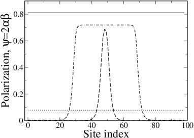
Figure 1: Polarization $\psi$ for $\delta/t_{0}=0.01$, $g/t_{0}=0.01$, $\chi/t_{0}=6$, $\rho_{P}=3\times 10^{-3}$ (dotted line), $\rho_{P}=6\times 10^{-3}$ (dashed line), $\rho_{P}=6\times 10^{-2}$ (dot-dashed line), and $\rho_{P}=10$ (solid line).

The results of the numerical solution for the function $\psi$ are shown in Fig. 1 for the case $\chi=6t_{0}$. At very low excitation densities $\rho_{P}=\frac{N_{P}}{N}$, where $N$ is the number of sites, polaritons behave as simple bosons. In that limit the self-trapping effect is absent since the nonlinear attractive potential is proportional to the local polariton density and can be neglected in this low density limit. Mathematically, this limit can be described by approximating $\frac{\psi}{\sqrt{1-\psi^{2}}}\approx\psi$ in the last term of Eq. (10). The cubic term $\psi^{3}$ is not strong enough to give rise to the self-trapping effect in this limit.

In the absence of the self-attractive term the distribution of the optical polarization is homogeneous. In this low excitation limit the chemical potential $\mu$ is simply given by

$$\mu=\frac{1}{2}(\omega^{\prime}_{X}+\omega_{c}-\sqrt{\delta^{2}+g^{\prime 2}})~{},$$ (16)

where $\omega^{\prime}_{X}=\omega_{X}-2t_{0}$ (energy at the bottom of the excitonic band), $\delta=\omega^{\prime}_{X}-\omega_{c}$ is the optical detuning, and $g^{\prime}=g\sqrt{N}$. Notice that in this limit the chemical potential does not depend on the coefficient of the cubic term in Eq. (10). Moreover in this limit the chemical potential corresponds to the energy of the lowest polariton at $k=0$.

VI.2 Intermediate density: self-trapping

By increasing the number of polaritons we observe a critical polariton number at which a symmetry-breaking transition occurs. A similar symmetry-breaking transition was found in the case of BEC with an attractive nonlinear interaction. carr00 Our numerical calculations for the dependence of $\mu$ on the polariton density $\rho_{P}=\frac{N_{P}}{N}$ are shown in Fig. 2 for several values of the cubic term $\chi$.

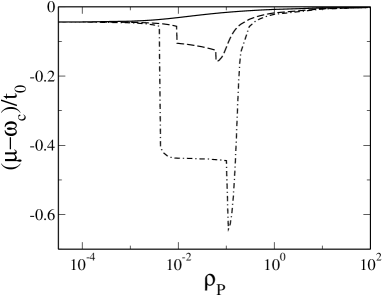
Figure 2: Polariton chemical potential as a function of the polariton density for $\delta/t_{0}=0.01$, $g/t_{0}=0.01$, $\chi/t_{0}=0$ (solid line), $\chi/t_{0}=4.5$ (dashed line), and $\chi/t_{0}=6$ (dot-dashed line).

When the exciton number increases following the polariton number, a self-trapping occurs, caused by the polariton-lattice coupling (dashed line in Fig. 1). There is a drop in the chemical potential at the point of symmetry-breaking (Fig. 2) due to the self-trapping. The breaking of the spatial homogeneity gives a negative contribution to the energy of the system. Also, this makes exciton-like states more energetically favorable than photon-like states, which results in a sharp decrease of the photonic component for nonzero $\chi$, as shown in Fig. 3. The self-trapping effect brings a discontinuity both in the chemical potential $\mu$, and in the photon (exciton) density as a function of the polariton density. Since the effective attractive potential depends on both $|\psi|^{2}$ and $\chi$, the point of symmetry breaking for higher $\chi$ corresponds to smaller values of the polariton density $\rho_{P}=\frac{N_{P}}{N}$.

Starting from the small excitation limit, we can expand $\frac{\psi}{\sqrt{1-\psi^{2}}}\approx\psi+\frac{1}{2}\psi^{3}$. The second term introduces an effective repulsion related to the intrinsic fermionic nature of the excitons and decreases the cubic term $\chi$ by $\frac{\omega_{X}-\mu}{2}$. Some analytical forms for the solution of Eq. (10a) with fixed exciton number can be written in terms of Elliptical functions. In particular, in the case when the photon number is much smaller than the exciton number, we can neglect the fourth term in Eq. (10a), since as seen from Eq. (10b), $\lambda$ is inversely proportional to $\omega_{c}-\mu$. In this limit the solution can be written in the form

$$\psi=A\mathrm{sech}[Y(\nu-\nu_{0})]~{},$$ (17)

where

$$Y=\frac{(\chi-\frac{\omega_{X}-\mu}{2})N_{P}}{4t_{0}}~{},$$ (18)

$$A=\sqrt{\frac{YN_{P}}{2}}~{},$$ (19)

and the chemical potential is determined by the equation

$$\mu=\omega_{X}-2t_{0}-\frac{(\chi-\frac{\omega_{X}-\mu}{2})^{2}N^{2}_{P}}{16t_{0}}~{}.$$ (20)

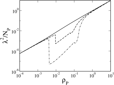
Figure 3: Photon density as a function of polariton density for $\chi/t_{0}=0$ (solid line), $\chi/t_{0}=4.5$ (dashed line), and $\chi/t_{0}=6$ (dot-dashed line).

VI.3 Saturation

By further increasing the polariton density, the internal fermionic structure of the excitons gives rise to a hard-core repulsion term, which leads to the saturation of the exciton states, making the polarization distribution broader and flatter at the top (dot-dashed line in Fig. 1). When the saturation spreads over the whole chain length, the polarization distribution (solid line in Fig. 1) becomes homogeneous again. We expect a discontinuity of $\mu$ again at this point as a consequence of the disappearance of the gradient of the polarization function (kinetic term), which gives a positive contribution to the energy. With the further increase of the exciton density the hopping effect is reduced due to the blocking. Fig. 4 shows half of the exciton density $\frac{\int|\beta|^{2}d\nu}{N}$ as a function of $\rho_{P}$, which reaches 1 in the limit of large excitation density regardless the value of $\chi$, corresponding to half filling of the exciton band. The half filling maximizes the polarization and hence minimizes the dipole interaction energy between the excitons and the cavity photons. In this saturation regime the polaritons become photon-like, since an added excitation mainly contributes to the cavity mode, and thus the chemical potential approaches $\omega_{c}$ (see also Fig. 2). A gradient in the density of polarization produces a force on the ions according to Eq. (8b). The force is stronger at the edges of the saturation region of the $|\psi|^{2}$ distribution as seen in Fig. 5, and is positive to the left from the center of the symmetry-breaking point and negative to the right. This reduces of the total length of the chain due to the interaction with the electromagnetic cavity mode.

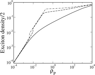
Figure 4: Half of exciton density as a function of the polariton density for $\chi/t_{0}=0$ (solid line), $\chi/t_{0}=4.5$ (dashed line), and $\chi/t_{0}=6$ (dot-dashed line).

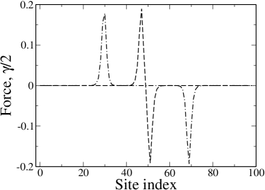
Figure 5: Force as a function of the site index for $\chi/t_{0}=6$, $\rho_{ex}=6\times 10^{-3}$ (dashed line), $\rho_{ex}=6\times 10^{-2}$ (dot-dashed line).

VII Homogeneous deformation and role of damping

The lattice deformation in the presence of optical excitations can be understood by analyzing the total energy of the system in the assumption that the lattice deformation is homogeneous. As seen in the previous section, this assumption is justified for a systems in the saturation regime or for a polariton density below the critical value for self-trapping. The total energy of the lattice is modified by the presence of polaritons. The homogeneous deformation allows us to obtain an analytical expression for the total energy of the system, and to analyze the effect of the finite linewidth of polaritons. We will include both the spontaneous emission of the excitons and the finite Q-factor of the cavity mode. Instead of using the variational approach of Sec. III, we will solve directly the equations of motion for the excitons and cavity photons.

We start by using the Fourier transform

$$B_{n}=\frac{1}{\sqrt{N}}\sum\limits_{k}e^{ikna}b_{k}~{},$$ (21)

where $N$ is the number of lattice sites, $k$ is the wave vector, and $a$ is the lattice separation, to define the operator $b_{k}$ as the annihilation operator of an exciton with a wave vector $k$. The Hamiltonian in Eq.  (1) can then be rewritten as

$$H=\sum\limits_{n}\left[\frac{p_{n}^{2}}{2M}+\frac{C}{2}\left(u_{n+1}-u_{n}\right)^{2}\right]+$$

$$+\sum\limits_{k}\omega_{k}b^{\dagger}_{k}b_{k}+\sum\limits_{k,k^{\prime}}f(k,k^{\prime})b^{\dagger}_{k}b_{k^{\prime}}$$

$$+\omega_{c}c^{\dagger}c+\frac{g^{\prime}}{2}c^{\dagger}b_{0}+\frac{g^{\prime}}{2}cb^{\dagger}_{0}~{},$$ (22)

where $\omega_{k}=\omega_{X}-2t_{0}\cos(ka)$ and

$$f(k,k^{\prime})=\frac{\gamma}{N}\sum\limits_{n}\left(u_{n+1}-u_{n}\right)\times$$

$$\times\left[e^{-ika}e^{ina(k-k^{\prime})}+e^{ik^{\prime}a}e^{ina(k^{\prime}-k)}\right]~{}.$$ (23)

We consider a finite-length chain with periodic boundary conditions. The equilibrium lattice displacement is homogeneous and will be indicated by $u=u_{n+1}-u_{n}$. Notice that in this limit $f(k,k^{\prime})$ is diagonal

$$f(k,k^{\prime})=2\gamma\cos(ka)u\delta_{k,k^{\prime}}~{}.$$ (24)

Eqs. (24) and  (22) show that in this homogeneous case there is no mixing of polariton with different $k$ vector. Since the cavity couples to the $k=0$ exciton mode only, the polariton modes at $k\neq 0$ are completely decoupled and do not enter in the dynamics. Taking into account Eq. (24), the excitonic part in $H$ reduces to $\omega_{0}(u)b_{0}^{\dagger}b_{0}$, where $\omega_{0}(u)=\omega_{X}-2t_{0}+2\gamma u$ is the energy of the exciton at $k=0$ renormalized by the lattice deformation potential. We also add a term that describes the pumping of the cavity mode by an external field and represent the full system by

$$H=\sum\limits_{n}\left[\frac{p_{n}^{2}}{2M}+\frac{Cu^{2}}{2}\right]+$$

$$+\omega_{0}(u)b_{0}^{\dagger}b_{0}+\frac{g^{\prime}}{2}(c^{\dagger}b_{0}+b_{0}^{\dagger}c)+\omega_{c}c^{\dagger}c+$$

$$\frac{\kappa E_{0}}{2}(ce^{i\omega_{c}t}+c^{\dagger}e^{-i\omega_{c}t})~{},$$ (25)

where $E_{0}$ represents the electric field of the external pump and $\kappa$ is the coupling between the external pump and the cavity mode. The operators $B_{n}$ are fermionic on the same site, but commute for different sites. Therefore, the commutation relation for $b_{0}$ reads

$$[b_{0},b_{0}^{\dagger}]=1-\frac{2\sum\limits_{n}B_{n}^{\dagger}B_{n}}{N}~{}.$$ (26)

Since we will assume here that there are no excitations of phonon modes at $k\neq 0$, we have that $\sum\limits_{N}B_{n}^{\dagger}B_{n}=\sum\limits_{k}b_{k}^{\dagger}b_{k}\sim b_{0}^{\dagger}b_{0}$. The equations for the expectation values of the polarization $\langle b_{0}\rangle=p$, exciton density $\langle b^{\dagger}_{0}b_{0}\rangle=n_{X}$ and cavity photon operator $\langle c\rangle=\lambda$ can be obtained using the standard factorization scheme axt94 and read

$$\dot{\lambda}=-i\left[\omega_{c}\lambda+\frac{g^{\prime}}{2}p+\frac{\kappa E_{0}}{2}e^{-i\omega_{c}t}\right]-\alpha_{c}\lambda~{},$$ (27)

$$\dot{p}=-i\left[\omega_{0}(1-\frac{2n_{X}}{N})p+\frac{g^{\prime}}{2}\lambda(1-\frac{2n_{X}}{N})\right]-\Gamma p~{},$$ (28)

$$\dot{n_{X}}=-i\frac{g^{\prime}}{2}(1-\frac{2n_{X}}{N})(p^{*}\lambda-p\lambda^{*})-2\Gamma n~{},$$ (29)

where we have introduced the spontaneous emission rate of the excitons $\Gamma$ and the damping of the cavity mode $\alpha_{c}$, due to the finite $Q$-factor of the cavity. The equation for $\lambda$ can be explicitly integrated and gives

$$i\lambda=\frac{g^{\prime}}{2}\frac{p}{\alpha_{c}}+\frac{\kappa E_{0}}{2\alpha_{c}}e^{-i\omega_{c}t}~{}.$$ (30)

This expression can be used in Eqs. (28) and  (29) which give for the steady state

$$\tilde{p}=\frac{-i\frac{g^{\prime}}{2}\frac{\kappa E_{0}}{2\alpha_{c}}(1-\frac{2n_{X}}{N})}{\omega_{c}-\omega_{0}(1-\frac{2n_{X}}{N})+i\Gamma+i\frac{g^{\prime 2}}{4\alpha_{c}}(1-\frac{2n_{X})}{N})}~{},$$ (31)

where we have defined $p=\tilde{p}e^{-i\omega_{c}t}$.

Figure 6: Effective lattice potential as a function of displacement. The figure has been obtained for the following set of parameters: $E_{g}=\omega_{X}-2t_{0}=2.282$ eV, $D=2\gamma a=6.1$ eV, $S=2.5\cdot 10^{3}$m/s, $a=1.5$ nm, $M=2.110^{-21}$ g, $\omega_{0}=2.282$ eV, and $C=S^{2}M/a^{2}=82eV/a^{2}$. The excitation corresponds to $\rho_{ex}\sim 0.1$. $\alpha_{c}=g^{\prime}=1$ meV, and $\omega_{c}=2.242$ eV. $\Gamma=400$ $\mu$eV and $\Gamma=700$ $\mu$eV for the upper and lower curve, respectively. The curves are displaced for clarity.

The $u$-dependent total potential energy $U(u)$ of the system can be obtained by substituting the solution for $p$, $\lambda$, and $n_{X}$ which depend on $u$, into the initial Hamiltonian(25). At weak excitation we obtain

$$U(u)\sim\frac{NC}{2}u^{2}+\omega_{0}(u)n_{X}(u)+$$

$$+\omega_{c}\left[\left(\frac{g^{\prime}}{2\alpha}\right)^{2}-\frac{2\Gamma}{\alpha_{c}}\right]n_{X}(u)+\omega_{c}I~{}$$ (32)

where $I=\left(\frac{\kappa E_{0}}{2\alpha_{c}}\right)^{2}$ and

$$n_{X}(u)\sim|p|^{2}=\frac{I(g^{\prime}/2)^{2}}{(\delta+2\gamma u)^{2}+\Gamma^{2}}~{}.$$ (33)

Notice that $n_{X}$ has a resonant behavior as a function of $u$, which is a consequence of the deformation potential shift in the excitonic energy.

In the absence of light the potential energy $U$ depends quadratically on $u$ with a minimum at $u=0$. When the laser is switched on, this dependence changes due to the presence of optical excitations in the system. Due to the resonant behavior in Eq.  (33), it is energetically favorable to have $u\neq 0$ if this reduces the total energy of the system. Figure  6 shows the potential energy for some values of parameters. The parameters used in these calculations are typical of polydiacetylene chains. We observe that the potential $U$ has a parabolic dependence with a superposed Lorentian contribution due to the optical excitation. This Lorentian contribution can be either positive or negative depending on the relative strength of the exciton-cavity coupling, spontaneous emission rate and cavity damping. The actual behavior can be explicitly calculated using Eq. (32). In the figure we consider two particular sets of parameters providing a minimum of the energy that corresponds to contraction and expansion of the lattice.

VIII Conclusion

In conclusions, we have investigated the optically-induced lattice strain in a single polymer chain in a cavity. We have extended the excitonic SSH model, describing the exciton propagation in the chain, to include the effect of the cavity electromagnetic field. Using a polariton picture, we have obtained a system of integro-differential nonlinear equations for the spatial distribution of the optical excitations in the chain. We find solutions describing a self-trapping of the polaritons which saturate when the excitation density is increased. The chemical potential of the polaritons shows a discontinuity at a threshold value of the polariton density. This critical density corresponds to the onset of the self-trapping. The self-trapping causes a sharp increase in the excitonic component and decrease in the photonic component of the polariton wavefunction. We have also considered the role of the finite radiative recombination rate of the excitons and the finite Q-factor of the cavity. These can be studied in a direct way in the case of a homogeneous strain field. We have found that both a contraction and expansion of the lattice are possible, depending of the relative strength of the exciton-cavity coupling, radiative recombination, and cavity Q-factor.

References

- (1) J. G. Müller, U. Lemmer, G. Raschke, M. Anni, U. Scherf, J. M. Lupton, and J. Feldmann, Phys. Rev. Lett. 91, 267401 (2003)
- (2) T. Guillet, J. Berréar, R. Grousson, J. Kovensky, C. Lapersonne-Meyer, M. Shott, and V. Voliotis, Phys. Rev. Lett. 87 087401 (2001).
- (3) F. Dubin, J. Berréar, R. Grousson, T. Guillet, C. Lapersonne-Meyer, M. Shott, and V. Voliotis, Phys. Rev. B 66 113202 (2002).
- (4) F. Dubin, R. Melet, T. Barisien, R. Grousson, L. Legrand, M. Shott, and V. Voliotis, Nature Physics 2 32 (2006).
- (5) A. J. Heeger, S. Kivelson, J. R. Schrieffer and W. P. Su, Rev. Mod. Phys. 60, 781 (1988).
- (6) E. G. Wilson, J. Phys. C 16 6739 (1983); ibidem 16 1039 (1983).
- (7) M. H. Szymanska and P. B. Littlewood, Solid State Commun. 124, 103 (2002).
- (8) Y. Toyozawa Optical Processes in Solids, Cambridge University Press, Cambridge (2003).
- (9) M. V. Katkov and C. Piermarocchi, Phys. Rev. B 73 033305 (2006).
- (10) V. M. Agranovich, M. Litinskaia, and D. G. Lidzey, Phys. Rev. B 67, 085311 (2003).
- (11) H. Deng, G. Weihs, C. Santori, J. Bloch, and Y. Yamamoto, Science 298 199 (2002).
- (12) H. Deng, G. Weihs, D. Snoke, J. Bloch, and Y. Yamamoto, Proc. Nat. Acad. Sci. 100 15318 (2003).
- (13) M. Saba et al., Nature 414, 731 (2001).
- (14) B. I. Greene, J. Orenstein, and S. Schmitt-Rink, Science 247 679 (1990); B. I. Greene et al., Phys. Rev. Lett. 61 325 (1988).
- (15) F. Dubin, J. Berréar, R. Grousson, M. Shott, and V. Voliotis, Phys. Rev. B 73 121302(R) (2006).
- (16) Polydiacetylenes, edited by D. Bloor and R. R. Chance, NATO Advanced Study Institute, Series B: Physics (Nijhoff, Dordrecht, 1985).
- (17) R. H. Dicke, Phys. Rev. 93, 99 (1954).
- (18) P. R. Eastham and P. B. Littlewood, Phys. Rev. B 64 235101 (2001).
- (19) I. Štich, R. Car, M. Parrinello, and S. Baroni, Phys. Rev. B 39 4997 (1989).
- (20) F. Dalfovo and S. Stringari, Phys. Rev. A 53, 2477 (1996).
- (21) L. D. Carr, C. W. Clark, and W. P. Reinhardt Phys. Rev. A 62, 063611 (2000); ibidem 62, 063610 (2000).
- (22) V. M. Axt and A. Stahl, Z. Phys. B 93, 195 (1994).