Renormalization group study of the Kondo problem at a junction of several Luttinger wires

Abstract

We study a system consisting of a junction of $N$ quantum wires, where the junction is characterized by a scalar $S$-matrix, and an impurity spin is coupled to the electrons close to the junction. The wires are modeled as weakly interacting Tomonaga-Luttinger liquids. We derive the renormalization group equations for the Kondo couplings of the spin to the electronic modes on different wires, and analyze the renormalization group flows and fixed points for different values of the initial Kondo couplings and of the junction $S$-matrix (such as the decoupled $S$-matrix and the Griffiths $S$-matrix). We generally find that the Kondo couplings flow towards large and antiferromagnetic values in one of two possible ways. For the Griffiths $S$-matrix, we study one of the strong coupling flows by a perturbative expansion in the inverse of the Kondo coupling; we find that at large distances, the system approaches the ferromagnetic fixed point of the decoupled $S$-matrix. For the decoupled $S$-matrix with antiferromagnetic Kondo couplings and weak inter-electron interactions, the flows are to one of two strong coupling fixed points in which all the channels are strongly coupled to each other through the impurity spin. But strong inter-electron interactions, with $K_{\rho}<N/(N+2)$, stabilize a multi-channel fixed point in which the coupling between different channels goes to zero. We have also studied the temperature dependence of the conductance at the decoupled and Griffiths $S$-matrices.

I I. Introduction

The area of molecular electronics has grown tremendously in recent years as a result of the drive towards smaller and smaller electronic devices mol . Molecular electronic circuits typically need multi-probe junctions. The first experimental growths of three-terminal nanotube junctions were not well controlled zhou ; more recently, new growth methods have been developed whereby uniform $Y$-junctions have been produced li ; kumar ; terrones . Transport measurements have also been carried out for the $Y$-junctions papad , as well as for three-terminal junctions obtained by merging together single-walled nanotubes by molecular linkers chiu .

On the theoretical side, there have been several studies of junctions of quantum wires. There have been detailed studies of carbon nanotubes with different proposed structures for the junction gan1 ; treboux . Several groups have analyzed the geometry and stability of the junctions menon ; meunier . Junctions of quantum wires have also been studied nayak ; chamon ; lal1 ; das ; chen ; meden in terms of one-dimensional wires, with the junction being modeled by a scattering matrix $S$. These studies include the effects of electron-electron interactions which are often cast in the language of Tomonaga-Luttinger liquid (TLL) theory gogolin ; rao ; giamarchi .

Many earlier studies of junctions have only included ‘scalar’ scatterings at the junction. i.e., the $S$-matrix has been taken to be spin-independent. The response of a junction of quantum wires to a magnetic impurity or an impurity spin at the junction has recently been studied both experimentally leturcq and theoretically rosch ; oreg ; pustilnik1 ; pustilnik2 ; ravi . As is well-known in three dimensions, an impurity spin can lead to the Kondo effect kondo . [The coupling between the conduction electrons and the impurity spin grows as one goes to lower temperatures; this leads to a larger scattering and therefore a larger resistance as long as the temperature is higher than the Kondo temperature $T_{K}$. Below $T_{K}$, the resistance due to scattering from the impurity spin decreases (if the value of the impurity spin $\cal S$ is larger than or equal to half the number of channels $N$) because the spin decouples from the electrons.] The Kondo effect for a ‘two-wire junction’ in a TLL wire has been studied by several groups lee ; furusaki ; fabrizio ; frojdh ; durga1 ; egger ; kim ; durga2 . Using a renormalization group (RG) analysis for weak potential scattering, Furusaki and Nagaosa showed that for an impurity spin of 1/2, there is a stable strong coupling fixed point (FP) consisting of two semi-infinite uncoupled TLL wires and a spin singlet furusaki . For strong potential scattering, the above FP is reached when the inter-electron interactions are weak. However, sufficiently strong inter-electron interactions are known to stabilize the two-channel Kondo FP instead fabrizio . The Kondo effect has also been studied in crossed TLL wires karyn and in multi-wire systems granath ; yi .

In this paper, we consider a junction of quantum wires which is characterized by an $S$-matrix at the junction; further, an impurity spin is coupled to the electrons at the junction. The wires are modeled as semi-infinite TLLs. The details of the model defined in the continuum will be described in Sec. II. In Sec. III, we will discuss how RG equations for the Kondo couplings and for the $S$-matrix at the junction can be obtained by successively integrating out the electronic modes far from the Fermi energy. We find that the flow of the Kondo couplings involve the $S$-matrix elements, but the flow of the $S$-matrix elements do not involve the Kondo couplings (up to second order in the latter). To simplify our analysis, therefore, we concentrate on the FPs of the $S$-matrix RG equations and study how the Kondo couplings evolve in Sec. IV. For the case of $N$ decoupled wires, we find that for a large range of initial values of the Kondo couplings, the system flows to a multi-channel ferromagnetic (FM) FP lying at zero coupling. This FP is associated with spin-flip scatterings of the electrons from the impurity spin whose temperature dependence will be discussed. Outside this range, the flow is towards a strong antiferromagnetic (AFM) coupling. On the other hand, at the Griffiths $S$-matrix (defined below), there is no stable FP for finite values of the Kondo couplings, and the system flows towards strong AFM coupling in two possible ways. We also consider the case when the scattering matrix has a chiral form. In this case, we find that the Kondo coupling matrix for the three wire case has three independent degrees of freedom and a single FP at strong coupling.

The strong coupling flows will be further discussed in Sec. V where we will consider some lattice models at the microscopic length scale. As in the three-dimensional Kondo problem, we find that there are various possibilities depending on the number of wires $N$ and the spin $\cal S$ of the impurity, such as the under-screened, over-screened and exactly screened cases noz1 . We will generally see that a Kondo coupling which is small at high temperatures (small length scales) can become large at low temperatures (large length scales). In Sec. VI, we will show that the vicinity of one of the strong coupling FPs can be studied through an expansion in the inverse of the coupling; we will then find that the large coupling can be re-interpreted as a small coupling in a different model.

In Sec. VII, we will study the case of decoupled wires with strong interactions using the technique of bosonization. Analogous to the results of fabrizio , we find that the multi-channel ($N\geq 2$) AFM Kondo FP is stabilized for $K_{\rho}<N/(N+2)$. We will discuss the temperature dependence of the conductance in Sec. VIII at both high and low temperature; we will compare the behaviors of Fermi liquids and TLLs. Sec. IX will contain some concluding remarks. A condensed version of some parts of this paper has appeared elsewhere ravi .

Before proceeding further, we would like to emphasize that we have not used bosonization in this paper (except in Sec. VII), although this is a powerful and commonly used method for studying TLLs gogolin ; rao ; giamarchi . In the presence of a junction with a general scattering matrix, it is not known whether the idea of bosonization can be implemented. (Some reasons for the difficulty in bosonizing are explained in Ref. lal1 ). It is therefore necessary to work directly in the fermionic language. We have adopted the following point of view in this work lal1 ; yue . We start with non-interacting electrons for which the scattering matrix approach and the Landauer formalism for studying electronic transport datta ; imry are justified. We then assume that the interactions between the electrons are weak, and treat the interactions to first order in perturbation theory to derive the RG equations. This is the approach used in most of this paper. Only in Sec. VII do we use bosonization to discuss the effect of strong interactions for the case of decoupled wires, since that is one of the cases where bosonization can be used.

II II. Model for several wires coupled to an impurity spin

We begin with $N$ semi-infinite quantum wires which meet at one site which is the junction; on each wire, the spatial coordinate $x$ will be taken to increase from zero at the junction to $\infty$ as we move far away from the junction.

The incoming and outgoing fields are related by an $S$-matrix at the junction, which is an $N\times N$ unitary matrix whose explicit values depend on the details of the junction. Hence the wave function corresponding to an electron with spin $\alpha$ ($\alpha=\uparrow,\downarrow$) and wave number $k$ which is incoming in wire $i$ ($i=1,2,\cdots,N$) is given by

$$\psi_{i\alpha k}(x) = e^{-i(k+k_{F})x}~{}+~{}S_{ii}e^{i(k+k_{F})x}~{}~{}{\rm on~{}wire~{}}i~{},$$ (1)

$$= S_{ji}~{}e^{i(k+k_{F})x}~{}~{}{\rm on~{}wire~{}}j\neq i~{}.$$

Here $k$ is the wave number with respect to the Fermi wave number $k_{F}$ (i.e., $k=0$ implies that the energy of the electron is equal to the Fermi energy $E_{F}$). We will take $k$ to go from $-\Lambda$ to $\Lambda$, where $\Lambda$ is a cut-off of the order of $k_{F}$; we will eventually only be interested in the long wavelength modes with $|k|\ll\Lambda$. We will use a linearized approximation for the dispersion relation so that the energy of an electron with wave number $k$ is given by $v_{F}k$ with respect to the Fermi energy; here $v_{F}$ is the Fermi velocity, and we are setting $\hbar=1$. In Eq. (1), we will refer to the waves going as $e^{-ikx}$ as the incoming part $\psi_{Ii\alpha k}$, and the waves going as $e^{ikx}$ as the outgoing part $\psi_{Oi\alpha k}$ or $\psi_{Oj\alpha k}$.

The second quantized annihilation operator corresponding to the wave function in Eq. (1) is given by

$$\Psi_{i\alpha k}(x)~{}=~{}c_{i\alpha k}~{}\psi_{i\alpha k}(x)~{},$$ (2)

where the wire index $i$ runs from 1 to $N$, and the total second quantized operator is given by

$$\Psi_{\alpha}(x)~{}=~{}\sum_{i}~{}\int_{-\Lambda}^{\Lambda}~{}\frac{dk}{2\pi}~{}c_{i\alpha k}~{}\psi_{i\alpha k}(x)~{}.$$ (3)

(Note that it is not possible to quantize the system in terms of $N$ independent fields on each of the wires, because an electron that is incoming on one wire has outgoing components on all the other wires as well). The non-interacting part of the Hamiltonian for the electrons is then given by

$$H_{0}~{}=~{}v_{F}~{}\sum_{i}~{}\sum_{\alpha}~{}\int_{-\Lambda}^{\Lambda}~{}\frac{dk}{2\pi}~{}k~{}c_{i\alpha k}^{\dagger}c_{i\alpha k}~{}.$$ (4)

If the impurity spin is coupled to the electrons at the junction, that part of the Hamiltonian is given by

$$H_{\rm spin}~{}=~{}\sum_{\alpha,\beta}~{}J~{}{\vec{S}}\cdot\Psi_{\alpha}^{\dagger}(x=0)~{}\frac{{\vec{\sigma}}_{\alpha\beta}}{2}\Psi_{\beta}(x=0)~{},$$ (5)

where ${\vec{\sigma}}$ denotes the Pauli matrices. (For simplicity, we will assume an isotropic spin coupling $J_{x}=J_{y}=J_{z}$). Eq. (5) can be written in terms of second quantized operators as

$$H_{\rm spin} = \sum_{i,j}\sum_{\alpha,\beta}~{}\int_{-\Lambda}^{\Lambda}~{}\int_{-\Lambda}^{\Lambda}~{}\frac{dk_{1}}{2\pi}~{}\frac{dk_{2}}{2\pi}$$ (6)

$$~{}~{}~{}~{}~{}~{}~{}~{}~{}~{}~{}~{}~{}J_{ij}~{}{\vec{S}}\cdot~{}c_{i\alpha k_{1}}^{\dagger}~{}\frac{{\vec{\sigma}}_{\alpha\beta}}{2}~{}c_{j\beta k_{2}}~{},$$

where $J_{ij}=J(1+\sum_{l}S_{li}^{*})(1+\sum_{m}S_{mj})$ is a Hermitian matrix. In general, however, the impurity spin may also be coupled to the electrons at other sites which are slightly away from the junction; for instance, this may be true if the model is defined on a lattice at the microscopic scale as we will see in Sec. V. It is therefore convenient to take $J_{ij}$ to be an arbitrary Hermitian matrix which is not necessarily related to the entries of the $S$-matrix in any simple way.

Next, let us consider density-density interactions between the electrons in each wire of the form (we will drop the wire index $i$ for the moment)

$$H_{\rm int}~{}=~{}\frac{1}{2}~{}\int\int~{}dx~{}dy~{}\rho(x)~{}U(x-y)~{}\rho(y)~{},$$ (7)

where the density $\rho$ is given in terms of the second quantized electron field $\Psi_{\alpha}(x)$ as $\rho=\Psi^{\dagger}_{\uparrow}\Psi_{\uparrow}+\Psi^{\dagger}_{\downarrow}\Psi_{\downarrow}$. As mentioned earlier for the wave-functions, the electron field can also be written in terms of outgoing and incoming fields as

$$\Psi_{\alpha}(x)~{}=~{}\Psi_{O\alpha}(x)~{}e^{ik_{F}x}~{}+~{}\Psi_{I\alpha}(x)~{}e^{-ik_{F}x}~{}.$$ (8)

If the range of the interaction $U(x)$ is short (of the order of the Fermi wavelength $2\pi/k_{F}$), such as that of a screened Coulomb repulsion, the Hamiltonian in (7) can be written as

$$H_{\rm int}=$$

$$\int dx\sum_{\alpha,\beta}[g_{1}\Psi_{O\alpha}^{\dagger}\Psi_{I\beta}^{\dagger}\Psi_{O\beta}\Psi_{I\alpha}+g_{2}\Psi_{O\alpha}^{\dagger}\Psi_{I\beta}^{\dagger}\Psi_{I\beta}\Psi_{O\alpha}$$

$$~{}~{}~{}~{}~{}~{}+\frac{1}{2}g_{4}(\Psi_{O\alpha}^{\dagger}\Psi_{O\beta}^{\dagger}\Psi_{O\beta}\Psi_{O\alpha}+\Psi_{I\alpha}^{\dagger}\Psi_{I\beta}^{\dagger}\Psi_{I\beta}\Psi_{I\alpha})],$$

(9)

where

$$g_{1}~{} = ~{}{\tilde{U}}(2k_{F})~{},$$

$${\rm and}~{}~{}~{}g_{2}~{} = ~{}g_{4}~{}=~{}{\tilde{U}}(0)~{}.$$ (10)

For repulsive and attractive interactions, $g_{2}>0$ and $<0$ respectively. (We have ignored umklapp scattering terms here; they only arise if the model is defined on a lattice and we are at half-filling).

III III. The renormalization group equations

It is known that the interaction parameters $g_{1}$, $g_{2}$ and $g_{4}$ satisfy some RG equations solyom ; the solutions of the lowest order RG equations are given by yue

$$g_{1}(L) = \frac{{\tilde{U}}(2k_{F})}{1~{}+~{}\frac{{\tilde{U}}(2k_{F})}{\pi v_{F}}\ln L}~{},$$

$$g_{2}(L) = {\tilde{U}}(0)~{}-~{}\frac{1}{2}~{}{\tilde{U}}(2k_{F})~{}+~{}\frac{1}{2}~{}\frac{{\tilde{U}}(2k_{F})}{1~{}+~{}\frac{{\tilde{U}}(2k_{F})}{\pi v_{F}}\ln L}~{},$$

$$g_{4}(L) = {\tilde{U}}(0)~{},$$ (11)

where $L$ denotes the length scale.

In general, the couplings $g_{1}$, $g_{2}$ and $g_{4}$ can have different values on different wires; hence we have to add a subscript $i$ to them. For weak interactions, i.e., when $g_{1i}$, $g_{2i}$ and $g_{4i}$ are all much less than $2\pi v_{F}$, we can derive the RG equations for the $S$-matrix at the junction yue ; lal1 . Let us define a parameter

$$\alpha_{i}~{}=~{}\frac{g_{2i}~{}-~{}2~{}g_{1i}}{2\pi v_{F}}~{},$$ (12)

which is a function of length scale due to Eqs. (11), and a diagonal matrix $M$ whose entries are given by

$$M_{ii}~{}=~{}\frac{1}{2}~{}\alpha_{i}r_{ii}~{}.$$ (13)

Then the RG equations can be written in the matrix form

$$\frac{dS}{d\ln L}~{}=~{}M~{}-~{}SM^{\dagger}S~{}.$$ (14)

The FPs of this equation are given by the condition $M=SM^{\dagger}S$.

Figure 1: Pictures of the terms which contribute to the renormalization of the Kondo coupling matrix $J$ to order $J^{2}$ and $g_{2}J$ respectively; $g_{2}$ denotes the coefficient of the electron-electron interaction. Thin lines and thick lines denote low energy and high energy electrons respectively.

We use the technique of ‘poor man’s RG’ anderson ; noz1 to derive the renormalization of the $S$-matrix and the Kondo coupling matrix $J_{ij}$. Briefly, this involves using the second order perturbation expression for the low energy effective Hamiltonian,

$$H_{\rm eff}~{}=~{}\sum_{h}~{}\frac{|l_{2}><l_{2}|H_{\rm pert}|h><h|H_{\rm pert}|l_{1}><l_{1}|}{E_{l}-E_{h}}~{},$$ (15)

where the perturbation $H_{\rm pert}$ is given by the sum of $H_{\rm spin}$ and $H_{\rm int}$ in Eqs. (6) and (9), $l_{1}$ and $l_{2}$ denote two energy states, and $h$ denotes high energy states. We now restrict the sum over $h$ in Eq. (15) to run over states for which the energy difference $E_{h}-E_{l}$ lies within an energy shell $E$ and $E+dE$; we have assumed that the difference between different low energy states is much smaller than $E$, so that we can simply write $E_{l_{1}}=E_{l}$ in the denominator of the above equation. We then see that the change in the effective Hamiltonian $dH_{\rm eff}$ is proportional to $dE/E$ which is equal to $-d\ln L$, where the length scale $L$ is inversely related to the energy scale $E$. In this way, we get an RG equation for the derivatives with respect to $\ln L$ of various parameters appearing in the low energy Hamiltonian.

Using this method, we find that the Kondo couplings $J_{ij}$ do not contribute to the renormalization of the $S$-matrix in Eq. (14) up to second order in $J_{ij}$. (This is not true beyond second order; however, we will only work to second order here assuming that the $J_{ij}$ are small). On the other hand, the $S$-matrix does contribute to the renormalization of the $J_{ij}$ through the interaction Hamiltonian in Eq. (9); this is because the relation between the outgoing field on wire $i$ (i.e., $\Psi_{Oi\alpha}$) and the operators $c_{j\alpha}$ involves the $S$-matrix. For instance, the terms involving $g_{2i}$ in Eq. (9) take the form

$$\sum_{i,j,l}\sum_{\alpha,\beta}~{}\int_{-\Lambda}^{\Lambda}~{}\int_{-\Lambda}^{\Lambda}~{}\int_{-\Lambda}^{\Lambda}~{}\int_{-\Lambda}^{\Lambda}~{}\frac{dk_{1}}{2\pi}~{}\frac{dk_{2}}{2\pi}~{}\frac{dk_{3}}{2\pi}~{}\frac{dk_{4}}{2\pi}$$

$$\times~{}\pi~{}\delta(k_{1}-k_{2}+k_{3}-k_{4})~{}g_{2i}$$

$$\times~{}S^{*}_{ij}c_{j\alpha k_{1}}^{\dagger}~{}c_{i\beta k_{2}}^{\dagger}~{}c_{i\beta k_{3}}~{}S_{il}c_{l\alpha k_{4}}~{},$$ (16)

where we have used the identity

$$\int_{0}^{\infty}~{}dx~{}e^{(-ik_{1}+ik_{2}-ik_{3}+ik_{4}-\epsilon)x}$$

$$=~{}-~{}\frac{i}{k_{1}-k_{2}+k_{3}-k_{4}-i\epsilon}$$

$$=~{}-~{}i~{}{\rm P}\Bigl{(}\frac{1}{k_{1}-k_{2}+k_{3}-k_{4}}\Bigr{)}$$

$$~{}~{}~{}~{}+~{}\pi~{}\delta(k_{1}-k_{2}+k_{3}-k_{4})~{},$$ (17)

with $\epsilon$ being an infinitesimal positive number. [In Eq. (16), we have kept only the $\delta$-function term and have dropped the principal part term since the latter can be either positive or negative, and its contribution vanishes when one integrates over the variables $k_{i}$.] Note that the terms involving $g_{2}$ in Eq. (16) (as well as those involving $g_{1}$ and $g_{4}$ in Eq. (9)) conserve momentum while the Kondo coupling terms in Eq. (6) do not.

We will omit the details of the RG calculations here apart from making a few comments below. We find that

$$\frac{dJ_{ij}}{d\ln L}$$

$$=~{}\frac{1}{2\pi v_{F}}~{}[~{}\sum_{k}~{}J_{ik}J_{kj}$$

$$~{}~{}~{}~{}+~{}\frac{1}{2}~{}g_{2i}~{}S_{ij}~{}\sum_{k}~{}J_{ik}S^{*}_{ik}~{}+~{}\frac{1}{2}~{}g_{2j}~{}S^{*}_{ji}~{}\sum_{k}~{}J_{kj}S_{jk}$$

$$~{}~{}~{}~{}-~{}\frac{1}{2}\sum_{k}~{}(g_{2k}-2g_{1k})~{}(J_{ik}S^{*}_{kk}S_{kj}+S^{*}_{ki}S_{kk}J_{kj})~{}]~{},$$

(18)

where $S_{ij}$ is the $S$-matrix at the length scale $L$. Eq. (18) is the key result of this paper. Note that it maintains the hermiticity of the matrix $J_{ij}$. Eq. (18) always has a trivial FP at $J_{ij}=0$.

Let us briefly comment on the origin of the various terms on the right hand side of Eq. (18). The first and second lines arise from Figs. 1 (a) and (b) respectively. (The terms of order $J^{2}$ in the first line have been derived in Ref. rosch ). The parameters $g_{1i}$ and $g_{4i}$ do not appear in the second line of Eq. (18) since the terms which are proportional to these parameters either do not appear in the numerator of Eq. (15) because they are not allowed by momentum conservation, or they appear in Eq. (15) but their contribution vanishes because the Pauli matrices are traceless. Finally, the third line of Eq. (18) arises as follows. In Ref. lal1 , the RG equation for the $S$-matrix was derived. This was based on the idea that due to reflections at the junction (these arise from the diagonal elements of the $S$-matrix which are the reflection amplitudes), there are Friedel oscillations in the density of the electrons; the amplitudes of these oscillations are proportional to $S_{kk}$ and $S^{*}_{kk}$ in wire $k$. We now treat the interactions in the Hartree-Fock approximation lal1 ; this results in reflections from the Friedel oscillations with a strength proportional to $g_{2k}-2g_{1k}$ in wire $k$. Now, an electron going from wire $j$ to $i$ can either (i) first go from wire $j$ to wire $k$ with a transmission amplitude $S_{kj}$, scatter from the Friedel oscillations in wire $k$ with an amplitude $(g_{2k}-2g_{1k})S^{*}_{kk}$, and finally scatter off the impurity spin from wire $k$ to wire $i$ with amplitude $J_{ik}$, or (ii) first scatter off the impurity spin from wire $j$ to wire $k$ with amplitude $J_{kj}$, scatter from the Friedel oscillations in wire $k$ with an amplitude $(g_{2k}-2g_{1k})S_{kk}$, and finally scatter from wire $k$ to wire $i$ with a transmission amplitude $S^{*}_{ki}$. These two processes give rise to the third line of Eq. (18).

It is interesting to observe that Eq. (18) remains invariant if we transform $S_{ij}\to e^{i\phi_{i}}S_{ij}$, where the $\phi_{i}$ can be arbitrary real numbers. According to Eq. (1), this corresponds to the freedom of redefining the phases of the outgoing waves by different amounts on different wires.

IV IV. Analysis of the renormalization group equations

To simplify our analysis, we will make two assumptions.

(i) The couplings $g_{1i}$ and $g_{2i}$ have the same value on all the wires, and therefore the subscript $i$ on $g_{1}$ and $g_{2}$ can be dropped.

(ii) The $S$-matrix is at a FP of Eq. (14), so that $S$ does not flow with the length scale.

We will now consider several possibilities for the $S$-matrix, and will study the RG flows and FPs of the Kondo couplings $J_{ij}$ in each case. The different possibilities can be realized in terms of quantum wires and quantum dots containing the impurity spin as shown in Fig. 2.

Figure 2: Schematic pictures of the system of wires (shown by solid lines), an impurity spin (shown inside a circle), and the coupling between the spin and the wires (dotted lines). Figures (a) and (b) show the cases of disconnected and Griffiths $S$-matrices respectively.

IV.1 A. $N$ disconnected wires

The $S$-matrix for $N$ disconnected wires is given by the $N\times N$ identity matrix (up to phases). (We will assume that $N\geq 2$). A picture of the system is indicated in Fig. 2 (a); the wires are disconnected from each other, and the end of each wire is coupled to the impurity spin. A more microscopic description of the system will be discussed in Sec. V.

Let us consider a highly symmetric form of the Kondo coupling matrix in which all the diagonal entries are equal to $J_{1}$ and all the off-diagonal entries are equal to $J_{2}$, with both $J_{1}$ and $J_{2}$ being real. (In the language of the three-dimensional $N$-channel Kondo problem, $J_{2}$ denotes coupling between different channels). Since the $S$-matrix is also symmetric under the exchange of any two of the $N$ indices, such a symmetric form of the Kondo matrix will remain intact during the course of the RG flow. In other words, it is natural for us to choose the $J$ matrix to have the same symmetry as the $S$-matrix, since that symmetry is preserved under the RG flow. Eq. (18) gives the two-parameter RG equations

$$\frac{dJ_{1}}{d\ln L} = \frac{1}{2\pi v_{F}}~{}[J_{1}^{2}+(N-1)J_{2}^{2}+2g_{1}J_{1}]~{},$$

$$\frac{dJ_{2}}{d\ln L} = \frac{1}{2\pi v_{F}}~{}[2J_{1}J_{2}+(N-2)J_{2}^{2}-(g_{2}-2g_{1})J_{2}]~{}.$$

(For $N=2$ and $g_{1}=0$, Eq. (LABEL:disc) agrees with the results in Ref. fabrizio ).

Since $g_{1}(L=\infty)=0$, Eq. (LABEL:disc) has only one FP at finite values of $(J_{1},J_{2})$, namely, the trivial FP at $(0,0)$. We then carry out a linear stability analysis around this FP. [Given a RG equation of the form $dX/d\ln L=aX$, we will say that the FP at $X=0$ is stable if $a<0$, unstable if $a>0$, and marginal if $a=0$. In the marginal case, we look at the next order term; if $dX/d\ln L=bX^{2}$ and $b>0$, we say that the FP at $X=0$ is stable on the $x<0$ side and unstable on the $x>0$ side.] If $\nu\equiv g_{2}(L=\infty)/(2\pi v_{F})>0$ (repulsive interactions), the stability analysis shows that the trivial FP is stable to small perturbations in $J_{2}$. For small perturbations in $J_{1}$, this FP is marginal; a second order analysis shows that it is stable if $J_{1}<0$ and unstable if $J_{1}>0$, i.e., it is the usual ferromagnetic FP which is found for Fermi liquid leads. However, the approach to the FP is quite different when the leads are TLLs. At large length scales, the FP is approached as $J_{1}\sim-1/\ln L$ and $J_{2}\sim 1/L^{\nu}$. From this, we can deduce the behavior at very low temperatures, namely,

$$J_{1}~{}\sim~{}-~{}1/\ln(T_{K}/T)~{},~{}~{}{\rm and}~{}~{}~{}J_{2}~{}\sim~{}(T/T_{K})^{\nu}~{}.$$ (20)

where we have introduced the Kondo temperature $T_{K}$. (This is given as usual by $T_{K}\sim\Lambda e^{-2\pi v_{F}/J}$, where $\Lambda$ is an energy cut-off of the order of the Fermi energy $E_{F}$, $J$ is the value of a typical Kondo coupling at the microscopic length scale as explained after Eq. (LABEL:asymp), and $1/(2\pi v_{F})$ is the density of states at $E_{F}$). The form in Eq. (20) is in contrast to the behavior of $J_{2}$ for Fermi liquid leads, i.e., for $g_{1}=g_{2}=0$. In that case, Eq. (LABEL:disc) can be solved exactly in terms of the linear combinations $J_{1}-J_{2}$ and $J_{1}+(N-1)J_{2}$; we again find a FP at $(J_{1},J_{2})=(0,0)$, with

$$J_{1}~{}\sim~{}-~{}1/\ln(T_{K}/T)~{},~{}~{}{\rm and}~{}~{}~{}J_{2}~{}\sim~{}1/\ln(T_{K}/T)^{2}~{}.$$ (21)

Note that $J_{2}$ approaches zero faster than $J_{1}$ for both Fermi liquid leads and TLL leads; but for the latter case, it goes to zero much faster, i.e., as a power of $T$.

Eq. (21) is valid provided that neither $J_{1}-J_{2}$ nor $J_{1}+(N-1)J_{2}$ is exactly equal to zero; if one of them is exactly zero and the other is not, then both $J_{1}$ and $J_{2}$ go as $1/\ln(T_{K}/T)$. However, having one of the two combinations exactly equal to zero requires a special tuning in a microscopic model, as we will see in Sec. V. In general, therefore, the powers of $1/\ln(T_{K}/T)$ in $J_{1}$ and $J_{2}$ are different; this does not seem to have been noted in the earlier literature.

Figure 3: RG flows of the Kondo couplings for three disconnected wires, with ${\tilde{U}}(0)={\tilde{U}}(2k_{F})=0.2(2\pi v_{F})$.

Figure 3 shows a picture of the RG flows for three wires for ${\tilde{U}}(0)={\tilde{U}}(2k_{F})=0.2(2\pi v_{F})$. [This gives a value of $\nu$ which is comparable to what is found in several experimental systems (see lal2 and references therein). In all the pictures of RG flows, the values of $J_{ij}$ are shown in units of $2\pi v_{F}$.] We see that the RG flows take a large range of initial conditions to the FP at $(0,0)$. For all other initial conditions, we see that there are two directions along which the Kondo couplings flow to large values; these are given by $J_{2}/J_{1}=1$ and $J_{2}/J_{1}=-1/(N-1)$ (with $N=3$). [On a cautionary note, we should remember that the RG equations studied here are only valid at the lowest order in $J_{ij}$ and $g_{2}$, i.e., for the case of weak repulsion (or attraction) and small Kondo couplings.]

The fact that the Kondo couplings flow to large values along two particular directions can be understood as follows. For values of $J_{1}$ and $J_{2}$ much larger than $g_{1}$ and $g_{2}$, one can ignore the terms of order $g_{1}$ and $g_{2}$ in Eq. (LABEL:disc). One then obtains the decoupled equations

$$\frac{d~{}[J_{1}-J_{2}]}{d\ln L} \simeq \frac{1}{2\pi v_{F}}~{}(J_{1}-J_{2})^{2}~{},$$

$$\frac{d~{}[J_{1}+(N-1)J_{2}]}{d\ln L} \simeq \frac{1}{2\pi v_{F}}~{}(J_{1}+(N-1)J_{2})^{2}~{}.$$

From these equations one can deduce that the couplings can flow to large values in one of two ways, depending on the initial conditions. Either $J_{1}+(N-1)J_{2}$ goes to $\infty$ much faster than $J_{1}-J_{2}$ (this is what happens in the first quadrant of the figures in Figs. 3 and 4), or $J_{1}-J_{2}$ goes to $\infty$ much faster than $J_{1}+(N-1)J_{2}$ (this happens in the fourth quadrant of the figures in Figs. 3 and 4). A third possibility is that $J_{2}$ remains exactly equal to zero while $J_{1}\to\infty$; however, this can only happen if one begins with $J_{2}$ exactly equal to zero. (This also seems to happen if the interactions are strong enough as we will discuss in Sec. VII). We will provide a physical interpretation of the first two possibilities in Sec. V.

Eq. (LABEL:asymp) has the form $dJ/d\ln L=J^{2}/(2\pi v_{F})$. If $J(d)$ denotes the value of $J$ at a microscopic length $d$, and $J(d)\ll 2\pi v_{F}$, then it becomes of order 1 at a length scale $L_{0}$ given by $L_{0}/d\sim e^{2\pi v_{F}/J(d)}$; the corresponding temperature is given by $T_{K}\sim\Lambda e^{-2\pi v_{F}/J(d)}$.

Finally, note that the special case with $J_{2}=0$ and $g_{1}=g_{2}=0$ is equivalent to the Kondo problem in three dimensions with $N$ channels and no coupling between channels kondo . In the three-dimensional case, the RG equation has been derived to fifth order in the Kondo coupling gan2 . This reveals a stable FP at a finite value of the coupling

$$J_{1}~{}=~{}\frac{4\pi v_{F}}{N}~{},$$ (23)

where $1/(2\pi v_{F})$ is the density of states at the Fermi energy. Thus the couplings $J_{ij}$ need not really flow to infinity as Fig. 3 would suggest; one may find strong coupling FPs lying at values of order $2\pi v_{F}$ if one takes into account terms of higher order in the RG equations. In Sec. VII, we do find a strong coupling FP for sufficiently strong inter-electron interactions.

Although we have discussed the case of completely disconnected wires here, the results do not change significantly if we allow a small spin-independent tunneling amplitude of the form

$$H_{\rm tun}~{}=~{}\tau~{}\sum_{i\neq j}~{}\sum_{\alpha}~{}\Psi_{i,\alpha}^{\dagger}(x_{i}=0)~{}\Psi_{j,\alpha}(x_{j}=0)~{}.$$ (24)

This is equivalent to changing the $S$-matrix slightly away from the identity matrix. Using the RG equation in (14), we find that the parameter $\tau$ satisfies the RG equation

$$\frac{d\tau}{d\ln L}~{}=~{}-~{}\frac{1}{2\pi v_{F}}~{}(g_{2}~{}-~{}2g_{1})~{}\tau~{}.$$ (25)

This has the same form as the interaction dependent terms in the RG equation for $J_{2}$ in (LABEL:disc). Hence, $\tau$ also scales at low temperatures as $T^{\nu}$ just like $J_{2}$ in Eq. (20). Thus the contributions of both $\tau$ and $J_{2}$ to the conductance go as $(T/T_{K})^{2\nu}$.

Here and subsequently we have not discussed the case of attractive interactions ($g_{2}<0$). The stability analysis can easily be suitably modified in that case; some of the directions for the RG flows may become stable and others may become unstable if the sign of $g_{2}$ is reversed.

IV.2 B. Griffiths $S$-matrix for $N$ wires

This is the case in which all the $N$ wires are connected to each other and there is maximal transmission, subject to the constraint that there is complete symmetry between the $N$ wires. (We will again assume that $N\geq 2$.) A picture of the system is indicated in Fig. 2 (b); the wires are connected to each other at a junction, and the junction is also coupled to the impurity spin. A more microscopic description of the junction will be discussed in Sec. V.

The maximally transmitting completely symmetric $S$-matrix is also called the Griffiths $S$-matrix and has all the diagonal entries equal to $-1+2/N$ and all the off-diagonal entries equal to $2/N$. Since here, too, the $S$-matrix is fully symmetric in the $N$ wires, we again consider the highly symmetric form of the Kondo coupling matrix as in the previous subsection, with real parameters $J_{1}$ and $J_{2}$ as the diagonal and off-diagonal entries respectively. Eq. (18) then gives

$$\frac{dJ_{1}}{d\ln L} = \frac{1}{2\pi v_{F}}~{}[J_{1}^{2}+(N-1)J_{2}^{2}~{}+~{}2g_{1}~{}(1-\frac{2}{N})^{2}~{}J_{1}$$

$$~{}~{}~{}~{}~{}~{}-~{}4g_{1}(1-\frac{2}{N})~{}(1-\frac{1}{N})~{}J_{2}~{}],$$

$$\frac{dJ_{2}}{d\ln L} = \frac{1}{2\pi v_{F}}~{}[2J_{1}J_{2}+(N-2)J_{2}^{2}~{}-~{}\frac{4g_{1}}{N}~{}(1-\frac{2}{N})J_{1}$$ (26)

$$~{}~{}~{}~{}~{}~{}+~{}(g_{2}-2g_{1}(1-\frac{2}{N})^{2})~{}J_{2}~{}].$$

(For $N=2$, i.e., a full line with an impurity spin coupled to one point on the line, Eq. (26) agrees with the equations derived in Ref. furusaki ).

The only FP of Eq. (26) is again the trivial FP at the origin. A linear stability analysis shows that this FP is unstable in one direction ($J_{2}$) and marginal in the other ($J_{1}$) for $g_{2}(L=\infty)>0$.

Figure 4 shows a picture of the RG flows for three wires for ${\tilde{U}}(0)={\tilde{U}}(2k_{F})=0.2(2\pi v_{F})$. We see that there is no stable FP at finite values of the couplings. The couplings flow to large values along one of the two directions $J_{2}/J_{1}=1$ and $J_{2}/J_{1}=-1/(N-1)$. The reason for this is the same as that explained around Eq. (LABEL:asymp) since the RG equations in (LABEL:disc) and (26) have the same form for large values of $J_{1}$ and $J_{2}$.

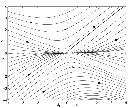
Figure 4: RG flows of the Kondo couplings for the Griffiths $S$-matrix for three wires, with ${\tilde{U}}(0)={\tilde{U}}(2k_{F})=0.2(2\pi v_{F})$.

IV.3 C. Chiral $S$-matrix for three wires

We choose a chiral $S$-matrix of the form

$$S = \left(\begin{array}[]{ccc}0&0&\gamma\\ \gamma&0&0\\ 0&\gamma&0\end{array}\right)~{},$$ (30)

where $\gamma$ is a complex number satisfying $|\gamma|=1$. (We will see a physical realization of this form in Sec. V. Alternatively, we could have considered an $S$-matrix which is the transpose of the one given above).

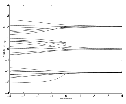
Figure 5: RG flows for the chiral $S$-matrix for three wires, with ${\tilde{U}}(0)={\tilde{U}}(2k_{F})=0.2(2\pi v_{F})$. The upper and lower figures show the magnitude and phase respectively of $J_{2}$.

Let us consider a Kondo coupling matrix of the form

$$J = \left(\begin{array}[]{ccc}J_{1}&J_{2}&J^{*}_{2}\\ J^{*}_{2}&J_{1}&J_{2}\\ J_{2}&J^{*}_{2}&J_{1}\end{array}\right)~{},$$ (34)

where $J_{1}$ is real but $J_{2}$ can be complex.

Then Eq. (18) gives

$$\frac{dJ_{1}}{d\ln L} = \frac{1}{2\pi v_{F}}~{}[~{}J_{1}^{2}+2|J_{2}|^{2}~{}]~{},$$

$$\frac{dJ_{2}}{d\ln L} = \frac{1}{2\pi v_{F}}~{}[~{}2J_{1}J_{2}+(J^{*}_{2})^{2}~{}+~{}\frac{1}{2}~{}g_{2}J_{2}~{}]~{}.$$ (35)

[Note that the above equations remain invariant under the transformation $J_{2}\to J_{2}e^{i2\pi/3}$ or $J_{2}e^{-i2\pi/3}$. We will see in Sec. V. C that a lattice realization of the chiral $S$-matrix has the same symmetry.]

One can again show that the only FP of Eq. (35) is the trivial FP at the origin. A linear stability analysis shows that the trivial FP is unstable in one direction ($J_{2}$) and marginal in the other ($J_{1}$) for $g_{2}(L=\infty)>0$. Figure 5 shows a picture of the RG flows for three wires for ${\tilde{U}}(0)={\tilde{U}}(2k_{F})=0.2(2\pi v_{F})$. The upper and lower figures show the way in which the magnitude and phase of $J_{2}$ evolve. We see that there is no stable FP at finite values of the couplings. The phase of $J_{2}$ flows towards one of the three values, 0 or $\pm 2\pi/3$; this is consistent with the symmetry of $J_{2}$ pointed out after Eq. (35). Further, $J_{1}$ and the magnitude of $J_{2}$ flow in such a way that $J_{1}+2|J_{2}|$ grows much faster than $J_{1}-|J_{2}|$. We can understand these observations as follows.

For values of $J_{1}$ and $J_{2}$ much larger than $g_{2}$, one can ignore the term of order $g_{2}$ in Eq. (35). If we write $J_{2}=|J_{2}|e^{i\phi}$, we find that

$$\frac{d\phi}{d\ln L} \simeq -~{}\frac{1}{2\pi v_{F}}~{}|J_{2}|~{}\sin(3\phi)~{},$$

$$\frac{d|J_{2}|}{d\ln L} \simeq \frac{1}{2\pi v_{F}}~{}[~{}2J_{1}|J_{2}|+|J_{2}|^{2}~{}\cos(3\phi)~{}]~{}.$$ (36)

The first equation in (36) shows that $\phi=0,\pm\pi/3,\pm 2\pi/3$ and $\pi$ are fixed points; however, since $|J_{2}|$ flows to $\infty$ under RG, only the values $\phi=0$ and $\pm 2\pi/3$ are stable. Substituting this fact that $\cos(3\phi)\to 1$ in the second equation in (36), and combining it with the first equation in (35), we obtain the decoupled equations

$$\frac{d~{}[J_{1}-|J_{2}|]}{d\ln L} \simeq \frac{1}{2\pi v_{F}}~{}(J_{1}-|J_{2}|)^{2}~{},$$

$$\frac{d~{}[J_{1}+2|J_{2}|]}{d\ln L} \simeq \frac{1}{2\pi v_{F}}~{}(J_{1}+2|J_{2}|)^{2}~{}.$$ (37)

From this we deduce that $J_{1}+2|J_{2}|$ must flow to $\infty$ much faster than $J_{1}-|J_{2}|$ since $J_{1}+2|J_{2}|>J_{1}-|J_{2}|$ to begin with. Note that unlike the disconnected and Griffiths cases, where $J_{1}$ and $J_{2}$ flow to large values in two possible ways (with $|J_{2}|/J_{1}\to 1$ and $-1/(N-1)$ respectively), in the chiral case, $J_{1}$ and $J_{2}$ flow to large values in only one way, along the direction $|J_{2}|/J_{1}=1$.

V V. Interpretation in terms of lattice models

We will now see how the different $S$-matrices and RG flows discussed in Sec. IV can be interpreted in terms of lattice models furusaki . This will provide us with physical interpretations of the various kinds of RG flows and FPs. We will concentrate on what the lattice models imply about the structure of the region near the junction, rather than the form of the interactions between the electrons in the bulk of the wires which has already been discussed in Sec. II. (The interactions can be introduced in the lattice model by, for instance, writing a Hubbard term at each site). We will again discuss three different cases here. (The models shown in Fig. 6 and discussed below in detail can be thought of as providing a microscopic picture of the systems shown in Fig. 2).

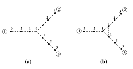
Figure 6: Lattice models for some of the $S$-matrices for three wires. (a) can be a model for the disconnected and Griffiths $S$-matrices, while (b) can be a model for the chiral $S$-matrix.

V.1 A. $N$ disconnected wires

This system can be realized by a lattice of the form shown in Fig. 6 (a). $N$ wires meet at a junction which is labeled by the site number 0; all the other sites are labeled as $n=1,2,\cdots$, with $n$ increasing as one goes away from the junction. (The lattice spacing will be set equal to one). We take the Hamiltonian to be of the tight-binding form, with a hopping amplitude equal to $-t$ on all the bonds (where $t$ is real), except for the bonds which connect the sites labeled as $n=1$ on each wire to the junction site; we set those hopping amplitudes equal to zero. This is equivalent to removing the junction site from the system; we will therefore not consider that site any further in this subsection. We then obtain a system of disconnected wires with an $S$-matrix which is equal to $-1$ times the identity matrix. To show this, we consider a wave which is incoming on wire $i$ with a wave number $k$, where $0<k<\pi$. We then find that the corresponding eigenstate of the Hamiltonian has an energy equal to $E_{k}=-2t\cos k$, and a wave function given by

$$\psi_{ik}(n) = e^{-ikn}~{}-~{}e^{ikn}~{}~{}{\rm for}~{}~{}n=1,2,\cdots~{}~{}{\rm on~{}wire~{}}i~{},$$

$$= 0~{}~{}{\rm at~{}the~{}junction~{}and~{}on~{}all~{}wires}~{}~{}j\neq i~{}.$$

We introduce an on-site potential which is equal to $\mu$ at all sites. In the absence of interactions, the ground state is one in which all the states with energies going from $=-2t$ up to $\mu$ are filled; the Fermi wave number $k_{F}$ is given by $\mu=-2t\cos k_{F}$, assuming that $\mu$ lies in the range $[-2t,2t]$. [We can then redefine all the wave numbers $k$ by subtracting $k_{F}$ from them as indicated after Eq. (1); the redefined wave numbers then run from $-\Lambda$ to $\Lambda$, where $\Lambda$ is of order $k_{F}$.]

Let us now consider coupling the impurity spin to the sites labeled as $n=1$ on the different wires by the following Hamiltonian

$$H_{\rm spin} = F_{1}~{}{\vec{S}}\cdot~{}\sum_{i}~{}\sum_{\alpha,\beta}~{}\Psi_{\alpha}^{\dagger}(i,1)~{}\frac{{\vec{\sigma}}_{\alpha\beta}}{2}~{}\Psi_{\beta}(i,1)$$

$$+~{}F_{2}~{}{\vec{S}}\cdot~{}\sum_{i\neq j}~{}\sum_{\alpha,\beta}~{}\Psi_{\alpha}^{\dagger}(i,1)~{}\frac{{\vec{\sigma}}_{\alpha\beta}}{2}~{}\Psi_{\beta}(j,1)~{},$$

where $\Psi_{\alpha}(i,1)$ denotes the second quantized electron field at site 1 on wire $i$ with spin $\alpha$. (Eq. (LABEL:heff2) below will provide a justification for this Hamiltonian). In Eq. (LABEL:hspin3), $F_{1}$ and $F_{2}$ denote amplitudes for spin-dependent scattering from the impurity within the same wire and between two different wires respectively. Namely, a spin-up electron coming in through one wire can get scattered by the impurity spin as a spin-down electron either along the same wire ($F_{1}$) or along a different wire ($F_{2}$). We then find that the Kondo coupling matrix $J_{ij}$ in Eq. (6) is as follows: all the diagonal entries are given by $J_{1}$ and all the off-diagonal entries are given by $J_{2}$, where

$$J_{1} = 4F_{1}\sin^{2}k_{F}~{},$$

$${\rm and}~{}~{}~{}J_{2} = 4F_{2}\sin^{2}k_{F}$$ (40)

for modes with redefined wave numbers lying close to zero. This is precisely the kind of Kondo matrix whose RG flows were studied in Sec. IV. A. The flows of the parameters $J_{1}$ and $J_{2}$ considered there can be translated into flows of the parameters $F_{1}$ and $F_{2}$ here. In particular, the approach to the FP at $(J_{1},J_{2})=(0,0)$ given by Eq. (20) at low temperatures implies that spin-flip scattering within the same wire or between two different wires will have quite different temperature dependences.

The flows to strong coupling shown in Fig. 3 can be interpreted as follows. In the first quadrant of Fig. 3, we see that $J_{1}+(N-1)J_{2}$ goes to $\infty$ faster than $|J_{1}-J_{2}|$; Eq. (40) then implies that $F_{1}$ and $F_{2}$ go to $\infty$. In the fourth quadrant of Fig. 3, $J_{1}-J_{2}$ goes to $\infty$ faster than $|J_{1}+(N-1)J_{2}|$; this implies that $F_{1}$ goes to $\infty$ and $F_{2}$ goes to $-\infty$ as $-F_{1}/(N-1)$.

These flows to strong coupling have the following interpretations. In the first case, $F_{1}$ and $F_{2}$ flow to $\infty$. From Eq. (LABEL:hspin3), this implies that the impurity spin (of magnitude $\cal S$) is strongly and antiferromagnetically coupled to only one electronic field, namely, the ‘centre of mass’ field given by $\sum_{i}\Psi(i,1)/\sqrt{N}$ (suppressing the spin labels and the Pauli matrices for the moment). Hence that field and the impurity spin will combine to form an effective spin of ${\cal S}-1/2$. In analogy with the three-dimensional Kondo problem, we can say that the impurity spin is under-screened or exactly screened if ${\cal S}>1/2$ or ${\cal S}=1/2$ respectively. In the second case, $F_{1}$ and $F_{2}=-F_{1}/(N-1)$ go to $\infty$. Using Eq. (LABEL:hspin3), we can then show that the impurity spin is strongly and antiferromagnetically coupled to the $N-1$ ‘difference’ fields (given by the orthogonal combinations $[\Psi(1,1)-\Psi(2,1)]/\sqrt{2}$, $[\Psi(1,1)+\Psi(2,1)-2\Psi(3,1)]/\sqrt{6},\cdots$). Hence those fields and the impurity spin will combine to give an effective spin of ${\cal S}-(N-1)/2={\cal S}+1/2-N/2$. Thus the impurity spin is under-screened, exactly screened or over-screened if $2{\cal S}+1$ is greater than, equal to or less than $N$ respectively.

V.2 B. Griffiths $S$-matrix for $N$ wires

This system can again be realized by the lattice shown in Fig. 6 (a) and a tight-binding Hamiltonian. However, we now take the hopping amplitude to be $-t$ on all bonds, except for the bonds which connect the sites labeled as $n=1$ on each wire to the junction site; on those bonds, we take the hopping amplitude to be $t_{1}=-t\sqrt{2/N}$. The on-site potential is taken to be $\mu$ at all sites, including the junction. We then find that the $S$-matrix is of the Griffiths form for all values of the wave number $k$. Namely, for a wave which is incoming on wire $i$ with a wave number $k$, the wave function is given by

$$\psi_{ik}(n) = e^{-ikn}~{}-~{}(1-\frac{2}{N})~{}e^{ikn}~{}~{}{\rm on~{}wire~{}}i~{},$$ (41)

$$= \frac{2}{N}~{}e^{ikn}~{}~{}{\rm on~{}all~{}wires}~{}~{}j\neq i~{},$$

$$= \frac{2}{N}~{}~{}{\rm at~{}the~{}junction~{}site}~{}.$$

We now consider coupling the impurity spin to the junction site labeled by zero, and the sites labeled as $n=1$ on the different wires by the following Hamiltonian

$$H_{\rm spin} = F_{3}~{}{\vec{S}}\cdot~{}\sum_{\alpha,\beta}~{}\Psi_{\alpha}^{\dagger}(0)~{}\frac{{\vec{\sigma}}_{\alpha\beta}}{2}~{}\Psi_{\beta}(0)$$

$$+~{}F_{4}~{}{\vec{S}}\cdot~{}\sum_{i}~{}\sum_{\alpha,\beta}~{}\Psi_{\alpha}^{\dagger}(i,1)~{}\frac{{\vec{\sigma}}_{\alpha\beta}}{2}~{}\Psi_{\beta}(i,1)~{},$$

where $\Psi_{\alpha}(0)$ denotes the second quantized electron field at the junction site with spin $\alpha$. (Sec. VI will provide a justification for this kind of a coupling). Then the Kondo coupling matrix $J_{ij}$ in Eq. (6) takes the following form: all the diagonal entries are given by $J_{1}$ and all the off-diagonal entries are given by $J_{2}$, where

$$J_{1} = \frac{4F_{3}}{N^{2}}~{}+~{}2F_{4}~{}[~{}1~{}-~{}(1-\frac{2}{N})\cos 2k_{F}~{}]~{},$$

$${\rm and}~{}~{}~{}J_{2} = \frac{4F_{3}}{N^{2}}~{}+~{}\frac{4F_{4}}{N}\cos 2k_{F}$$ (43)

for modes with wave numbers lying close to zero. The RG flows of this kind of Kondo matrix were studied in Sec. IV. B.

In terms of $F_{3}$ and $F_{4}$, the variables in Eq. (LABEL:asymp) are given by

$$J_{1}~{}-~{}J_{2} = 2F_{4}~{}(1-\cos 2k_{F})~{},$$

$${\rm and}~{}~{}~{}J_{1}+(N-1)J_{2} = \frac{4F_{3}}{N}~{}+~{}2F_{4}~{}(1+\cos 2k_{F})~{}.$$

Since $0<k_{F}<\pi$, $1\pm\cos 2k_{F}$ lie between 0 and 2. In the first quadrant of Fig. 4, $J_{1}+(N-1)J_{2}$ goes to $\infty$ faster than $|J_{1}-J_{2}|$; Eq. (LABEL:jab2) then implies that $F_{3}$ goes to $\infty$ and $|F_{4}|\ll F_{3}$. In the fourth quadrant of Fig. 4, $J_{1}-J_{2}$ goes to $\infty$ faster than $|J_{1}+(N-1)J_{2}|$; this implies that $F_{4}$ goes to $\infty$ and $F_{3}$ goes to $-\infty$.

These flows to strong coupling have the following interpretations. In the first case, $F_{3}$ flows to $\infty$ which means that the impurity spin (of magnitude $\cal S$) is strongly and antiferromagnetically coupled to an electron spin at the junction site $n=0$; hence those two spins will combine to form an effective spin of ${\cal S}-1/2$. (This case will be discussed in detail in Sec. VI). In the second case, $F_{3}$ goes to $-\infty$ while $F_{4}$ goes to $\infty$; hence the impurity spin is coupled strongly and ferromagnetically to an electron spin at the site $n=0$, and antiferromagnetically to electron spins at the sites labeled as $n=1$ on each of the $N$ wires (see Fig. 6 (a) for the site labels). Hence the impurity spin will combine with those $N+1$ spins to form an effective spin of ${\cal S}+1/2-N/2$. Interestingly, we see that the magnitudes of the effective spins formed in the strong coupling limits in the first and fourth quadrants are the same in the cases of $N$ disconnected wires and the Griffiths $S$-matrix.

V.3 C. Chiral $S$-matrix for three wires

This system can be realized by a lattice of the form shown in Fig. 6 (b). The three wires meet at a triangle; the sites on each wire are labeled as $n=1,2,\cdots$. The hopping amplitude is taken to be $-t$ on all the bonds, except for the three bonds on the triangle. On those bonds, we take the hopping amplitude to be complex, and of the form $-te^{i\theta}$ in the clockwise direction and $-te^{-i\theta}$ in the anticlockwise direction. [We can think of the total phase $3\theta$ of the product of hopping amplitudes around the triangle as being the Aharonov-Bohm phase arising from a magnetic flux enclosed by the triangle. Such a flux breaks time reversal symmetry which makes the $S$-matrix non-symmetric. Note that since only the value of $3\theta$ modulo $2\pi$ has any physical significance, we are free to shift the value of $\theta$ by $\pm 2\pi/3$. This changes the phase of the coupling $J_{2}$ defined below.] We then find that the $S$-matrix is of the chiral form given by Eq. (30), provided that the wave number $k$ satisfies

$$e^{i(3\theta+k)}~{}=~{}-~{}1~{}.$$ (45)

The phase $\gamma$ in (30) is then given by $e^{i(\theta+k)}$. [Unlike the disconnected and Griffiths cases, we have not found a lattice model which gives an $S$-matrix as in (30) for all values of the wave number $k$.] Given a value of $\theta$, we therefore choose a chemical potential $\mu=-2t\cos k_{F}$ such that $k_{F}$ satisfies Eq. (45). Since the properties of a fermionic system at low temperatures are governed by the modes near $k_{F}$, the above prescription produces a system with a chiral $S$-matrix.

We now consider coupling the impurity spin to the three sites of the triangle through the Hamiltonian

$$H_{\rm spin} = ~{}F_{5}~{}{\vec{S}}\cdot~{}\sum_{i}~{}\sum_{\alpha,\beta}~{}\Psi_{\alpha}^{\dagger}(i,1)~{}\frac{{\vec{\sigma}}_{\alpha\beta}}{2}~{}\Psi_{\beta}(i,1)~{}.$$

Then the Kondo coupling matrix $J_{ij}$ in Eq. (6) takes the form given in Eq. (34), where

$$J_{1} = 2F_{5}~{},$$

$${\rm and}~{}~{}~{}J_{2} = F_{5}e^{-i(\theta+3k_{F})}$$ (47)

for modes with wave numbers lying close to zero. This is a special case of the Kondo matrix given in Eq. (34). [To obtain the most general form given in (34), we need to introduce another parameter, such as a coupling of the impurity spin to the sites labeled by $n=2$ in Fig. 6 (b).] The RG flows of this kind of Kondo matrix were studied in Sec. IV. C.

VI VI. Expansion around a strong coupling fixed point

In Sec. V, we considered several examples of $S$-matrices and the RG flows of the Kondo coupling. In most cases, we found that the Kondo couplings flow to large values. We can now ask whether the vicinity of the strong coupling FPs can be studied in some way. We will see that it is possible to do so through an expansion in the inverse of the Kondo coupling noz1 .

We will consider one example of such an expansion here. Following the discussion given after Eq. (LABEL:jab2), let us assume that the RG flows for the case of the Griffiths $S$-matrix have taken us to a strong coupling FP along the direction $J_{2}/J_{1}=1$, as shown in the first quadrant of Fig. 4. This implies that the coupling of the impurity spin $S$ to an electron spin at the junction site $n=0$ has a large and positive (antiferromagnetic) value $F_{3}$, while its coupling to the sites labeled as $n=1$ on each of the wires has a finite value $F_{4}$ which is much less than $F_{3}$ (the site labels are shown in Fig. 6 (a)). The ground state of the $F_{3}$ term (namely, just the first term in Eq. (LABEL:hspin4)) consists of a single electron at site $n=0$ which forms a total spin of ${\cal S}-1/2$ with the impurity spin. The energy of this spin state is $-F_{3}({\cal S}+1)/2$; this lies far below the high energy states in which there is a single electron at site $n=0$ which forms a total spin of ${\cal S}+1/2$ with the impurity spin (these states have energy $F_{3}{\cal S}/2$), or the states in which the site $n=0$ is empty or doubly occupied (these states have zero energy).

We can now do a perturbative expansion in $1/F_{3}$. We take the unperturbed Hamiltonian to be one in which the hopping amplitudes on all the bonds are $-t$, except for the bonds connecting the sites labeled as $n=1$ on the different wires to the junction site; we take those hopping amplitudes to be zero. (This means that the unperturbed Hamiltonian corresponds to the case of $N$ disconnected wires). We also include the spin coupling proportional to $F_{3}$ in the unperturbed Hamiltonian. We take the perturbation $H_{\rm pert}$ as consisting of (i) the hopping amplitude $t_{1}$ on the bonds connecting the sites labeled as $n=1$ to the junction site, and (ii) the $F_{4}$ term in Eq. (LABEL:hspin4). Using this perturbation, we can find an effective Hamiltonian noz1 . [Once again, we use the expression in Eq. (15), where the high energy states are the ones listed in the previous paragraph. We will work up to second order in $t_{1}$ and $F_{4}$.] If ${\cal S}>1/2$, we find that the effective Hamiltonian has no terms of order $t_{1}$ or $t_{1}F_{4}$, and it is given by

$$H_{\rm eff} = F_{\rm 1,eff}~{}{\vec{S}}_{\rm eff}\cdot~{}\sum_{i}~{}{\vec{s}}_{i}$$

$$+~{}F_{\rm 2,eff}~{}{\vec{S}}_{\rm eff}\cdot\sum_{i\neq j}~{}\sum_{\alpha,\beta}~{}\Psi^{\dagger}_{\alpha}(i,1)~{}\frac{{\vec{\sigma}}_{\alpha\beta}}{2}~{}\Psi_{\beta}(j,1)$$

$$+~{}C~{}\sum_{i\neq j}~{}({\vec{S}}_{\rm eff}\cdot{\vec{s}}_{i})~{}({\vec{S}}_{\rm eff}\cdot{\vec{s}}_{j})~{}+~{}D~{}\sum_{i<j}{\vec{s}}_{i}\cdot{\vec{s}}_{j}$$

plus some constants, where

$${\vec{s}}_{i} = \sum_{\alpha,\beta}~{}\Psi_{\alpha}^{\dagger}(i,1)~{}\frac{{\vec{\sigma}}_{\alpha\beta}}{2}~{}\Psi_{\beta}(i,1)~{},$$

$$F_{\rm 1,eff} = -~{}\frac{8~{}t_{1}^{2}}{({\cal S}+1)~{}(2{\cal S}+1)~{}F_{3}}~{}+~{}\frac{2({\cal S}+1)F_{4}}{2{\cal S}+1}$$

$$-~{}\frac{2~{}({\cal S}+1)~{}F_{4}^{2}}{(2{\cal S}+1)^{3}~{}F_{3}}~{},$$

$$F_{\rm 2,eff} = -~{}\frac{8~{}t_{1}^{2}}{({\cal S}+1)~{}(2{\cal S}+1)~{}F_{3}}~{},$$

$$C = \frac{2~{}F_{4}^{2}}{(2{\cal S}+1)^{3}~{}F_{3}}~{},$$

$${\rm and}~{}~{}~{}D = -~{}\frac{F_{4}^{2}}{(2{\cal S}+1)~{}F_{3}}~{}.$$ (49)

In Eq. (LABEL:heff2), ${\vec{S}}_{\rm eff}$ denotes an object with spin ${\cal S}-1/2$. We thus find a weak interaction between the spin ${\cal S}-1/2$ and all the sites which are nearest neighbors of the site $n=0$ as shown in Fig. 6 (a).

If the impurity is a spin-1/2 object (i.e., ${\cal S}=1/2$), then the electron at the site $n=0$ forms a singlet with the impurity. In that case, only the last term in Eq. (LABEL:heff2) survives. However, there are other terms in the effective Hamiltonian which are of higher order in $t_{1}/F_{3}$ than in (LABEL:heff2); these have been calculated in Ref. noz2 for the case ${\cal S}=1/2$. One of these terms describes spin-independent tunneling from one wire to another, of the form $\sum_{i\neq j}\sum_{\alpha}\Psi^{\dagger}_{\alpha}(i,1)\Psi_{\alpha}(j,1)$. This is a contribution to the $S$-matrix at the junction, and it can contribute to the conductance from one wire to another as we will discuss in Sec. VIII.

Returning to the case ${\cal S}>1/2$, we note that the last two terms in Eq. (LABEL:heff2) are irrelevant as boundary operators if $g_{2}(L=\infty)/(2\pi v_{F})$ is small; this is because ${\vec{s}}_{i}$ has the scaling dimension $1-g_{2}/(2\pi v_{F})$ (as one can see from Eq. (LABEL:disc)), and therefore the product ${\vec{s}}_{i}\otimes{\vec{s}}_{j}$ has the scaling dimension $2(1-g_{2}/(2\pi v_{F}))$ which is larger than $1$. The first two terms in Eq. (LABEL:heff2) have the same form as in Eqs. (LABEL:hspin3) and (40), where the effective Kondo couplings

$$J_{\rm 1,eff} = 4F_{\rm 1,eff}~{}\sin^{2}k_{F}~{},$$

$${\rm and}~{}~{}~{}J_{\rm 2,eff} = 4F_{\rm 2,eff}~{}\sin^{2}k_{F}$$ (50)

are equal, negative and small. We can now study the RG flow of this as in Sec. IV. A. With these initial conditions, Eq. (LABEL:disc) and Fig. 3 show that the Kondo couplings flow to the FP at $(J_{\rm 1,eff},J_{\rm 2,eff})=(0,0)$.

In this example, therefore, we obtain a picture of the RG flows at both short and large length scales. We start with the Griffiths $S$-matrix with certain values of the Kondo coupling matrix, and we eventually end at the stable FP of the disconnected $S$-matrix for repulsive interactions, $g_{2}(L=\infty)>0$.

We will not discuss here what happens for the other possible RG flow for the Griffiths $S$-matrix, in which $J_{1}$ and $J_{2}$ become large along the direction $J_{2}/J_{1}=-1/(N-1)$. As we noted in Sec. V B, $N+1$ spins get coupled strongly to the impurity spin in that case; an expansion in the inverse coupling is much more involved in that case. For the same reason, we will not discuss expansions in the inverse coupling for the flows to strong coupling for the disconnected and chiral $S$-matrices.

VII VII. Decoupled wires with strong interactions

In this section, we will briefly discuss what happens if there are $N$ decoupled wires and the interactions are strong. For the decoupled $S$-matrix, one can ‘unfold’ the electron field in each semi-infinite wire to obtain a chiral electron field in an infinite wire, and then bosonize that chiral field gogolin ; rao ; giamarchi . In the language of bosonization, the interaction parameters are given by $K_{\rho}$ for the charge sector and $K_{\sigma}$ for the spin sector. Spin rotation invariance implies that $K_{\sigma}=1$, while $K_{\rho}$ is related to our parameters $g_{i}$ as follows giamarchi ,

$$K_{\rho} = \sqrt{\frac{1~{}+~{}g_{4}/\pi v_{F}~{}+~{}(g_{1}-2g_{2})/2\pi v_{F}}{1~{}+~{}g_{4}/\pi v_{F}~{}-~{}(g_{1}-2g_{2})/2\pi v_{F}}}$$ (51)

$$\to ~{}1~{}+~{}\frac{g_{1}-2g_{2}}{2\pi v_{F}}~{}.$$

In the second line of the above equation, we have taken the limit of small $g_{i}$ since we have worked to lowest order in the $g_{i}$ in the earlier sections. From Eq. (11), we see that $2g_{2}-g_{1}$ is invariant under the RG flow. The case of repulsive interactions corresponds to $2g_{2}-g_{1}>0$, i.e., $K_{\rho}<1$.

The case of two decoupled wires ($N=2$) has been studied by Fabrizio and Gogolin in Ref. fabrizio . They showed that if the interactions are weak enough, the Kondo couplings $J_{1}$ and $J_{2}$ are both relevant; their results then agree with those discussed in Sec. IV A. But if the interactions are sufficiently strong, i.e., $K_{\rho}<1/2$, then $J_{2}$ is irrelevant and flows to zero.

We will now show that their results can be generalized to the case of $N$ wires; one finds that there is again a value of $K_{\rho}$ below which $J_{2}$ is irrelevant. Following Ref. fabrizio , we can write the spin-up and down Fermi fields $\Psi_{i,\alpha}$ in wire $i$ in terms of the charge and spin bosonic fields $\Phi_{i,\rho}$ and $\Phi_{i,\sigma}$. Close to the junction denoted as $x_{j}=0$, we have

$$\Psi_{i,\uparrow} \sim \frac{\eta_{i,\uparrow}}{\sqrt{2\pi d}}~{}e^{i(\Phi_{i,\rho}/\sqrt{2K_{\rho}}~{}+~{}\Phi_{i,\sigma}/\sqrt{2})}~{},$$

$${\rm and}~{}~{}~{}\Psi_{i,\downarrow} \sim \frac{\eta_{i,\downarrow}}{\sqrt{2\pi d}}~{}e^{i(\Phi_{i,\rho}/\sqrt{2K_{\rho}}~{}-~{}\Phi_{i,\sigma}/\sqrt{2})}~{},$$ (52)

where we have used the fact that $K_{\sigma}=1$, and we have not explicitly written the arguments of the fields ($x_{i}=0$) for notational convenience. The $\eta_{i,a}$ denote Klein factors, and $d$ is a short distance cut-off; these will not play any role below.

In bosonic language, the Hamiltonian $H=H_{0}+H_{\rm int}$ in Eqs. (4) and (9) is given by

$$H~{}=~{}\frac{1}{4\pi}~{}\sum_{i}~{}\int_{0}^{\infty}~{}dx_{i}~{}[~{}v_{\rho}\left(\frac{\partial\Phi_{i,\rho}}{\partial x_{i}}\right)^{2}~{}+~{}v_{\sigma}\left(\frac{\partial\Phi_{i,\sigma}}{\partial x_{i}}\right)^{2}]~{},$$ (53)

where $v_{\rho}$, $v_{\sigma}$ denote the charge and spin velocities respectively. The bosonic fields satisfy the commutation relations

$$[~{}\frac{\partial\Phi_{i,a}(x_{i})}{\partial x_{i}}~{},~{}\Phi_{j,b}(x_{j})~{}]~{}=~{}i~{}2\pi~{}\delta_{ab}~{}\delta_{ij}~{}\delta(x_{i}~{}-~{}x_{j})~{},$$ (54)

where $a,b=\rho,\sigma$.

The impurity spin part of the Hamiltonian is given by

$$H_{\rm spin} = ~{}J_{1}~{}{\vec{S}}\cdot~{}\sum_{i}~{}\sum_{\alpha,\beta}~{}\Psi_{i,\alpha}^{\dagger}~{}\frac{{\vec{\sigma}}_{\alpha\beta}}{2}~{}\Psi_{i,\beta}$$ (55)

$$+~{}J_{2}~{}{\vec{S}}\cdot~{}\sum_{i\neq j}~{}\sum_{\alpha,\beta}~{}\Psi_{i,\alpha}^{\dagger}~{}\frac{{\vec{\sigma}}_{\alpha\beta}}{2}~{}\Psi_{j,\beta}~{}.$$

The spin densities on different wires are given by

$$\frac{1}{2}~{}[~{}\Psi_{i,\uparrow}^{\dagger}\Psi_{i,\uparrow}~{}-~{}\Psi_{i,\downarrow}^{\dagger}\Psi_{i,\downarrow}~{}]~{}=~{}\frac{1}{2\sqrt{2}\pi}~{}\frac{\partial\Phi_{i,\sigma}}{\partial x_{i}}~{}.$$ (56)

The other terms take the form

$$\Psi_{i,\uparrow}^{\dagger}\Psi_{i,\downarrow} \sim e^{-i\sqrt{2}\Phi_{i,\sigma}}~{},$$

$$\Psi_{i,\uparrow}^{\dagger}\Psi_{j,\uparrow} \sim e^{(i/\sqrt{2})[-\Phi_{i,\rho}/\sqrt{K_{\rho}}-\Phi_{i,\sigma}+\Phi_{j,\rho}/\sqrt{K_{\rho}}+\Phi_{j,\sigma}]~{}}~{},$$

$$\Psi_{i,\uparrow}^{\dagger}\Psi_{j,\downarrow} \sim e^{(i/\sqrt{2})[-\Phi_{i,\rho}/\sqrt{K_{\rho}}-\Phi_{i,\sigma}+\Phi_{j,\rho}/\sqrt{K_{\rho}}-\Phi_{j,\sigma}]~{}}~{},$$

and so on. In (55) and (LABEL:psi2), we have not explictly written the arguments of the fields, $x_{i}=x_{j}=0$; we will continue to do this wherever convenient. [The bosonic forms of the fermion bilinears in Eqs. (56) and (LABEL:psi2) are so different because we are using abelian bosonization. For the same reason, we will find it useful to distinguish between the different components of $J_{1}$ and $J_{2}$, i.e., $J_{1z}$, $J_{1\perp}$, $J_{2z}$, and $J_{2\perp}$.] Let us define $N$ ‘orthonormal’ linear combinations of the spin boson fields, namely, the ‘centre of mass’ combination

$$\Phi^{0}_{\sigma}~{}=~{}\frac{1}{\sqrt{N}}~{}\sum_{i}~{}\Phi_{i,\sigma}~{},$$ (58)

and the ‘difference’ fields

$$\Phi^{n}_{\sigma}~{}=~{}\frac{1}{\sqrt{n(n+1)}}~{}[~{}\sum_{m=1}^{n}~{}\Phi_{m,\sigma}~{}-~{}n~{}\Phi_{n+1,\sigma}~{}]~{},$$ (59)

where $n=1,2,\cdots,N-1$. We can now write Eq. (55) in the bosonic language. We obtain

$$H_{\rm spin} = \frac{J_{1z}}{2\sqrt{2}\pi}~{}S^{z}~{}\sum_{i}~{}\frac{\partial\Phi_{i,\sigma}}{\partial x_{i}}$$

$$+\frac{J_{1\perp}}{4\pi d}~{}[~{}S^{+}~{}e^{i\sqrt{2/N}\Phi^{0}_{\sigma}}~{}\sum_{i}~{}e^{i\sum_{n}a^{n}_{i}\Phi^{n}_{\sigma}}~{}+~{}H.c.]$$

$$-\frac{J_{2z}}{\pi d}~{}S^{z}~{}\sum_{i<j}~{}\sin\left(\sum_{n}b^{n}_{ij}\Phi^{n}_{\sigma}\right)~{}$$

$$~{}~{}~{}~{}~{}~{}~{}~{}~{}~{}~{}~{}~{}~{}\times~{}\sin\left(\frac{\Phi_{i,\rho}-\Phi_{j,\rho}}{\sqrt{2K_{\rho}}}\right)$$

$$+\frac{J_{2\perp}}{2\pi d}~{}[~{}S^{+}~{}e^{i\sqrt{2/N}\Phi^{0}_{\sigma}}~{}$$

$$~{}\times\sum_{i<j}~{}e^{i\sum_{n}c^{n}_{ij}\Phi^{n}_{\sigma}}\cos\left(\frac{\Phi_{i,\rho}-\Phi_{j,\rho}}{\sqrt{2K_{\rho}}}\right)+H.c.],$$

where the sums over $n$ in the second, third and last lines run over the ‘difference’ fields $\Phi^{n}_{\sigma}$. The constants $a^{n}_{i}$, $b^{n}_{ij}$ and $c^{n}_{ij}$ in Eq. (LABEL:hspin7) satisfy the relations

$$\sum_{n}~{}(a^{n}_{i})^{2} = 2~{}-~{}\frac{2}{N}~{},$$

$$\sum_{n}~{}(b^{n}_{ij})^{2} = 1~{},$$

$${\rm and}~{}~{}~{}\sum_{n}~{}(c^{n}_{ij})^{2} = 1~{}-~{}\frac{2}{N}$$ (61)

for all values of $i,j$.

We can remove the phase factors $\exp(i\sqrt{2/N}\Phi^{0}_{\sigma})$ in Eq. (LABEL:hspin7) by performing an unitary transformation of the total Hamiltonian $H_{\rm tot}$ given by the sum of (53) and (55), namely, $H_{\rm tot}\to UH_{\rm tot}U^{\dagger}$ emery , where

$$U~{}=~{}e^{-iS^{z}\sqrt{2/N}\Phi^{0}_{\sigma}}~{}.$$ (62)

After this transformation, Eq. (LABEL:hspin7) takes the form

$$H_{\rm spin} = \frac{\lambda}{2\sqrt{2}\pi}~{}S^{z}~{}\sum_{i}~{}\frac{\partial\Phi_{i,\sigma}}{\partial x_{i}}$$ (63)

$$+\frac{J_{1\perp}}{4\pi d}~{}[~{}S^{+}~{}\sum_{i}~{}e^{i\sum_{n}a^{n}_{i}\Phi^{n}_{\sigma}}~{}+~{}H.c.~{}]$$

$$-\frac{J_{2z}}{\pi d}~{}S^{z}~{}\sum_{i<j}~{}\sin\left(\sum_{n}b^{n}_{ij}\Phi^{n}_{\sigma}\right)~{}$$

$$~{}~{}~{}~{}~{}~{}~{}~{}~{}~{}~{}~{}~{}~{}\times~{}\sin\left(\frac{\Phi_{i,\rho}-\Phi_{j,\rho}}{\sqrt{2K_{\rho}}}\right)$$

$$+\frac{J_{2\perp}}{2\pi d}~{}[~{}S^{+}\sum_{i<j}~{}e^{i\sum_{n}c^{n}_{ij}\Phi^{n}_{\sigma}}\cos\left(\frac{\Phi_{i,\rho}-\Phi_{j,\rho}}{\sqrt{2K_{\rho}}}\right)$$

$$~{}~{}~{}~{}~{}~{}~{}~{}~{}~{}+~{}H.c.~{}]~{},$$

where $\lambda=J_{1z}-4\pi v_{\sigma}/N$. We can now study the problem in the vicinity of the point $\lambda=J_{1\perp}=J_{2z}=J_{2\perp}=0$. Note that this is a strong coupling FP, since $\lambda=0$ implies that

$$J_{1z}~{}=~{}\frac{4\pi v_{\sigma}}{N}~{}.$$ (64)

Since the scaling dimension of $e^{i\beta\Phi_{i,a}}$ is given by $\beta^{2}/2$, for $a=\rho,\sigma$, we see from Eq. (61) that the operators multiplying $J_{1\perp},J_{2z}$ and $J_{2\perp}$ in Eq. (63) have the scaling dimensions $1-1/N$, $1/2+1/(2K_{\rho})$ and $1/2-1/N+1/(2K_{\rho})$ respectively. This impies that the $J_{1\perp}$ operator is always relevant, while the $J_{2z}$ operator is irrelevant if $K_{\rho}<1$ (repulsive interactions). Most interestingly, the $J_{2\perp}$ operator is relevant or irrelevant depending on whether $K_{\rho}>$ or $<N/(N+2)$. For $N=2$, this gives the critical value of $K_{\rho}$ to be 1/2 fabrizio , while for $N\to\infty$, the critical value of $K_{\rho}$ approaches 1, i.e., the limit of weak repulsive interactions.

We saw in Sec. IV A that a flow to strong coupling is indeed possible along the line $J_{2}=0$, although that line is unstable to small perturbations in $J_{2}$. We now see that the line is stabilized (to first order in the couplings) if the interactions are sufficiently strong, i.e., if

$$K_{\rho}~{}<~{}\frac{N}{N+2}~{}.$$ (65)

If $J_{2}$ flows to zero and $J_{1}$ flows to large values, Eq. (LABEL:hspin3) shows that the impurity spin is coupled strongly and antiferromagnetically to the electron fields $\Psi(i,1)$ on all the $N$ wires; hence they will combine to form an effective spin of ${\cal S}-N/2$. (If ${\cal S}<N/2$, the impurity spin is over-screened). This describes a $N$-channel AFM FP with no coupling between channels oreg ; pustilnik2 .

VIII VIII. Conductance calculations

Our calculations for the Kondo couplings can be explicitly applied to various geometries of quantum wires and a quantum dot (containing the impurity spin) shown in Fig. 2, such as (a) a dot coupled independently to each wire (disconnected $S$-matrix for the wires), so that the conductance can only occur through the dot, or (b) a side-coupled dot (Griffiths $S$-matrix for the wires), where the conductance can occur directly between the wires. In general, of course, one can have any $S$-matrix at the junction, so that the conductance can occur both through the dot and directly between the wires.

Let us now consider the conductance near the different FPs durga2 ; pustilnik1 for the case of weak interactions. In the Griffiths case where the conductance can occur directly between the wires, let us consider the case of small values of $J_{1},J_{2}$ (both much smaller than $2\pi v_{F}$), and $g_{2}\gg g_{1}$. At high temperatures, before the $J_{i}$’s have grown very much under RG, we see from Eq. (26) that $J_{1}$ remains small, while $J_{2}$ grows due to the term $g_{2}J_{2}$. Namely, $J_{2}\sim(T/T_{K})^{-\nu}$, where $\nu=g_{2}(L=\infty)/(2\pi v_{F})$. The effect of $J_{2}$ is to scatter the electrons from the impurity spin, and thereby reduce the conductance between any two wires from the maximal value of $G_{0}=(4/N^{2})e^{2}/h$. Since the scattering probability is proportional to $J_{2}^{2}$, the conductance at high temperatures ($T\gg T_{K}$) is given by

$$G~{}-~{}G_{0}~{}\sim~{}-~{}G_{0}~{}{\cal S}({\cal S}+1)~{}(T/T_{K})^{-2\nu}~{}.$$ (66)

[The factor of ${\cal S}({\cal S}+1)$ appears for the following reason. Consider an electron coming in through wire $i$; it can have spin up or down, and the impurity spin can have any value of $S^{z}$ from ${\cal S}$ to $-{\cal S}$. We assign all these $2(2{\cal S}+1)$ states the same probability. As a result of the Kondo coupling $J_{2}$, the electron can scatter to a different wire $j$; as a result, its spin may or may not flip, and the value of $S^{z}$ for the impurity spin can also change by 0 or $\pm 1$. If we calculate the probabilities of all the different possible processes and add them, we get a factor of ${\cal S}({\cal S}+1)$]. Using Eq. (51), we see that (66) takes the form

$$G~{}-~{}G_{0}~{}\sim~{}-~{}G_{0}~{}{\cal S}({\cal S}+1)~{}(T/T_{K})^{K_{\rho}-1}~{},$$ (67)

where we have used the RG flow to set $g_{1}=0$ and $\nu=g_{2}(L=\infty)/(2\pi v_{F})$. On the other hand, if the leads were Fermi liquids ($g_{1}=g_{2}=0$), $J_{2}$ would be given by Eq. (21), and we would get

$$G~{}-~{}G_{0}~{}\sim~{}-~{}\frac{G_{0}{\cal S}({\cal S}+1)}{\ln(T/T_{K})^{4}}~{}.$$ (68)

At low temperatures, the Kondo couplings flow to large values; as discussed at the end of Sec. VI, their behaviors are then governed by the FP at $(J_{1,{\rm eff}},J_{2,{\rm eff}})=(0,0)$ of the disconnected wire case with an effective spin ${\cal S}_{\rm eff}={\cal S}-1/2$. In this case, only $J_{2}^{2}$ contributes to the conductance between two different wires. From Eq. (20), we see that the conductance is given by

$$G \sim G_{0}~{}{\cal S}_{\rm eff}({\cal S}_{\rm eff}+1)~{}(T/T_{K})^{2\nu}$$ (69)

$$\sim G_{0}~{}{\cal S}_{\rm eff}({\cal S}_{\rm eff}+1)~{}(T/T_{K})^{1-K_{\rho}}$$

for $T\ll T_{K}$. For Fermi liquid leads, Eq. (21) implies that the conductance is given by

$$G~{}\sim~{}\frac{G_{0}{\cal S}_{\rm eff}({\cal S}_{\rm eff}+1)}{\ln(T/T_{K})^{4}}~{}.$$ (70)

Thus a measurement of the temperature dependence of the conductance should be able to distinguish between the Fermi liquid and TLL cases at both high and low temperatures. For the case $N=2$, the expressions in Eqs. (67) and (69) agree with those given in Refs. furusaki ; durga2 , but Eqs. (68) and (70) differ from the expressions given in earlier papers (like Ref. durga2 ) for the powers of $1/\ln(T/T_{K})$. (As we had discussed earlier after Eq. (21), we would get the same powers of $1/\ln(T/T_{K})$ as in Ref. durga2 if $J_{2}$ was exactly equal to $J_{1}$ or $-J_{1}/(N-1)$).

The above expressions for the conductance shows that for both Fermi liquid leads and TLL leads (with repulsive interactions), and for both $T\gg T_{K}$ and $T\ll T_{K}$, the conductance increases with the temperature. It is then natural to assume that this would be true for intermediate temperatures as well, so that the conductance increases monotonically with temperature from 0 to $G_{0}$; this would be consistent with the results in Refs. furusaki ; durga2 . It may be useful to discuss here why there is no Kondo resonance peak in the conductance at low temperatures in our model, in contrast to what is found in other models (for instance Refs. pustilnik1 ; glazman ; ng ) and observed experimentally goldhaber ; wiel . In our model, once the impurity spin gets very strongly coupled to the junction site in Fig. 6 (b) (due to the flow to large $J_{1}$ and $J_{2}$ in the Griffiths case), that site decouples from the wires; this leaves no other pathway for the electrons to transmit from one wire to another. In contrast to this, if the junction region was more complicated (for instance, if there were additional bonds which connect different wires without going through the impurity spin, or there was a dot with several energy levels through which the electron can transmit), then the electron may still be able to transmit even after the impurity quenches the electron on a single site (or level). Hence, it may be possible for the conductance to increase to the unitarity limit at the lowest temperatures; this is known to occur for models with Fermi liquid leads. For TLL leads, however, our analysis remains valid even if there are additional bonds between the wires, because any such direct tunneling amplitudes are irrelevant and renormalize to zero as shown in Eq. (25).

Finally, let us briefly consider the case of strong inter-electron interactions. For $K_{\rho}<N/(N+2)$, we saw in Sec. VII that a multi-channel FP gets stabilized in the case of $N$ disconnected wires. To obtain the conductance at this point, we need to study the operators perturbing this point, similar to the analysis in Refs. pustilnik2 ; kim ; durga2 ; this has not yet been done.

IX IX. Conclusions

To summarize our results, we have studied systems of TLL wires which meet at a junction. The junction is described by a spin-independent $S$-matrix, and there is an impurity spin which is coupled isotropically to the electrons in the neighborhood of the junction. The $S$-matrix and the Kondo coupling matrix $J_{ij}$ satisfy certain RG equations. We have studied the RG flows of the Kondo couplings for a variety of FPs of the $S$-matrices. Although the Kondo couplings generally grow large, one can sometimes study the system through an expansion in the inverse of the coupling. This leads to a new system in which the effective Kondo couplings are weak; the RG flows of these effective couplings can then be studied.

For example, at the fully connected or Griffiths $S$-matrix, we find that for a range of initial conditions, the Kondo couplings can flow to a strong coupling FP along the direction $J_{2}/J_{1}=1$, where their fate is decided by a $1/J$ analysis. This analysis then shows that the couplings flow to the FM FP of the disconnected $S$-matrix lying at $(J_{1,{\rm eff}},J_{2,{\rm eff}})=(0,0)$. For this system, therefore, one obtains a description of the system at both short and large length scales.

For the case of disconnected wires and repulsive interactions, there is a range of Kondo couplings which flow towards a multi-channel FM FP at $(J_{1},J_{2})=(0,0)$. At low temperatures, we find spin-flip scattering processes with temperature dependences which are dictated by both the Kondo effect and the inter-electron interactions. It may be possible to observe such scatterings by placing a quantum dot with a spin at a junction of several wires with interacting electrons.

For other initial conditions for the disconnected case, the Kondo couplings flow towards the strong coupling FPs at $J_{1},|J_{2}|\to\infty$. In general, this is just the single channel strong coupling AFM FP. But there is a special line where $J_{1}\to\infty$ and $J_{2}=0$; this is the multi-channel AFM FP. The RG equations show that both $J_{1}$ and $J_{2}$ are relevant around the weak coupling FP if the interactions are weak. However, if the interactions are sufficiently strong (i.e., $K_{\rho}<N/(N+2)$), we find that $J_{2}\to 0$, and the multi-channel FP gets stabilized.

Experiments are underway to look for multi-channel FPs, and proposals have been made for minimizing the couplings between channels using gate voltages oreg . We suggest here that enhancing inter-electron interactions in the wires offers another way of reducing the inter-channel coupling and thereby observing the effects of the multi-channel FP.

Finally, we have discussed the temperature dependences of the conductances close to the disconnected and Griffiths $S$-matrices, and showed that this also provides a way to distinguish between Fermi liquid leads and TLL leads.

Acknowledgments

S.R. thanks P. Durganandini for discussions. V.R.C thanks CSIR, India for financial support. V.R.C. and D.S. thank DST, India for financial support under the project No. SP/S2/M-11/2000.

References

- (1)
- (2) G. Cuniberti, G. Fagas, and K. Richter, eds., Introducing Molecular Electronics (Springer, Berlin, 2005).
- (3) D. Zhou and S. Seraphin, Chem. Phy. Lett. 238, 286 (1995).
- (4) J. Li, C. Papadapoulos, and J. Xu, Nature 402, 253 (1999).
- (5) B. C. Satish Kumar, P. J. Thomas, A. Govindaraj, and C. N. R. Rao, Appl. Phys. Lett. 77, 2530 (2000).
- (6) M. Terrones, F. Banhart, N. Grobert, J.-C. Charlier, H. Terrones, and P. M. Ajayan, Phys. Rev. Lett. 89, 075505 (2002).
- (7) C. Papadopoulos, A. Rakitin, J. Li, A. S. Vedeneev, and J. M. Xu, Phys. Rev. Lett. 85, 3476 (2000).
- (8) P.-W. Chiu, M. Kaempgen, and S. Roth, Phys. Rev. Lett. 92, 246802 (2004).
- (9) B. Gan, J. Ahn, Q. Zhang, Q.-F. Huang, C. Kerlit, S. F. Yoon, Rusli, V. A. Ligachev, X.-B. Zhang, and W.-Z. Li, Materials Lett. 45, 315 (2000).
- (10) G. Treboux, P. Lapstun, and K. Silverbrook, Chem. Phy. Lett. 306, 402 (1999).
- (11) M. Menon and D. Srivastava, Phys. Rev. Lett. 79, 4453 (1997); M. Menon, A. N. Andriotis, D. Srivastava, I. Ponomareva, and L. Chernozatonskii, Phys. Rev. Lett. 91, 145501 (2003).
- (12) V. Meunier, M. B. Nardelli, J. Bernholc, T. Zacharia, and J. -C. Charlier, Appl. Phys. Lett. 81, 5234 (2002).
- (13) C. Nayak, M. P. A. Fisher, A. W. W. Ludwig, and H. H. Lin, Phys. Rev. B59, 15694 (1999).
- (14) C. Chamon, M. Oshikawa, and I. Affleck, Phys. Rev. Lett. 91, 206403 (2003); M. Oshikawa, C. Chamon, and I. Affleck, J. Stat. Mech.: Theory Exp. 2006, 0602 (2006) P008, cond-mat/0509675.
- (15) S. Lal, S. Rao, and D. Sen, Phys. Rev. B66, 165327 (2002).
- (16) S. Das, S. Rao, and D. Sen, Phys. Rev. B70, 085318 (2004).
- (17) S. Chen, B. Trauzettel, and R. Egger, Phys. Rev. Lett. 89, 226404 (2002); R. Egger, B. Trauzettel, S. Chen, and F. Siano, New Journal of Physics 5, 117 (2003).
- (18) X. Barnabe-Theriault, A. Sedeki, V. Meden, and K. Schönhammer, Phys. Rev. B71, 205327 (2005), and Phys. Rev. Lett. 94, 136405 (2005).
- (19) A. O. Gogolin, A. A. Nersesyan, and A. M. Tsvelik, Bosonization and Strongly Correlated Systems (Cambridge University Press, Cambridge, 1998).
- (20) S. Rao and D. Sen, in Field Theories in Condensed Matter Physics, edited by S. Rao (Hindustan Book Agency, New Delhi, 2001).
- (21) T. Giamarchi, Quantum Physics in One Dimension (Oxford University Press, Oxford, 2004).
- (22) R. Leturcq, L. Schmid, K. Ensslin, Y. Meir, D. C. Driscoll, and A. C. Gossard, Phys. Rev. Lett. 95, 126603 (2005).
- (23) A. Rosch, J. Paaske, J. Kroha, and P. Wölfle, J. Phys. Soc. Jpn. 74, 118 (2005); N. Shah and A. Rosch, cond-mat/0509680.
- (24) Y. Oreg and D. Goldhaber-Gordon, Phys. Rev. Lett. 90, 136602 (2003).
- (25) M. Pustilnik and L. Glazman, J. Phys. Condens. Matter 16, R513 (2004).
- (26) M. Pustilnik, L. Borda, L. I. Glazman, and J. von Delft, Phys. Rev. B69, 115316 (2004).
- (27) V. Ravi Chandra, S. Rao, and D. Sen, cond-mat/0510206, to appear in Europhys. Lett. (2006).
- (28) A. C. Hewson, The Kondo Problem to Heavy Fermions (Cambridge University Press, Cambridge, 1993).
- (29) D.-H. Lee and J. Toner, Phys. Rev. Lett. 69, 3378 (1992).
- (30) A. Furusaki and N. Nagaosa, Phys. Rev. Lett. 72, 892 (1994).
- (31) M. Fabrizio and A. O. Gogolin, Phys. Rev. B51, 17827 (1995).
- (32) P. Fröjdh and H. Johannesson, Phys. Rev. B53, 3211 (1996).
- (33) P. Durganandini, Phys. Rev. B53, R8832 (1996).
- (34) R. Egger and A. Komnik, Phys. Rev. B57, 10620 (1998).
- (35) E. H. Kim, cond-mat/0106575.
- (36) P. Durganandini and P. Simon, cond-mat/0607237.
- (37) K. Le Hur, Phys. Rev. B61, 1853 (2000).
- (38) M. Granath and H. Johannesson, Phys. Rev. B57, 987 (1998).
- (39) H. Yi and C. L. Kane, Phys. Rev. B57, R5579 (1998); H. Yi, Phys. Rev. B65, 195101 (2002).
- (40) P. Nozieres and A. Blandin, J. Phys. (Paris) 41, 193 (1980).
- (41) D. Yue, L. I. Glazman, and K. A. Matveev, Phys. Rev. B49, 1966 (1994); K. A. Matveev, D. Yue, and L. I. Glazman, Phys. Rev. Lett. 71, 3351 (1993).
- (42) S. Datta, Electronic transport in mesoscopic systems (Cambridge University Press, Cambridge, 1995).
- (43) Y. Imry, Introduction to Mesoscopic Physics (Oxford University Press, New York, 1997).
- (44) J. Solyom, Adv. Phys. 28, 201 (1979).
- (45) P. W. Anderson, J. Phys. C 3, 2436 (1970).
- (46) S. Lal, S. Rao, and D. Sen, Phys. Rev. Lett. 87, 026801 (2001), and Phys. Rev. B65, 195304 (2002).
- (47) J. Gan, N. Andrei, and P. Coleman, Phys. Rev. Lett. 70, 686 (1993); J. Gan, J. Phys. Condens. Matter 6, 4547 (1994).
- (48) P. Nozieres, J. Low. Temp. Phys. 17, 31 (1974).
- (49) V. J. Emery and S. Kivelson, Phys. Rev. B46, 10812 (1992).
- (50) L. I. Glazman and M. E. Raikh, JETP Lett. 47, 452 (1988).
- (51) T. K. Ng and P. A. Lee, Phys. Rev. Lett. 61, 1768 (1988).
- (52) D. Goldhaber-Gordon, H. Shtrikman, D. Mahalu, D. Abusch-Magder, U. Meirav, and M. A. Kastner, Nature 391, 156 (1998).
- (53) W. G. van der Wiel, S. De Franceschi, T. Fujisawa, J. M. Elzerman, S. Tarucha, and L. P. Kouwenhoven, Science 289, 2105 (2000).