Flow transitions in two-dimensional foams

Abstract

For sufficiently slow rates of strain, flowing foam can exhibit inhomogeneous flows. The nature of these flows is an area of active study in both two-dimensional model foams and three dimensional foam. Recent work in three-dimensional foam has identified three distinct regimes of flow [S. Rodts, J. C. Baudez, and P. Coussot, Europhys. Lett. 69, 636 (2005)]. Two of these regimes are identified with continuum behavior (full flow and shear-banding), and the third regime is identified as a discrete regime exhibiting extreme localization. In this paper, the discrete regime is studied in more detail using a model two dimensional foam: a bubble raft. We characterize the behavior of the bubble raft subjected to a constant rate of strain as a function of time, system size, and applied rate of strain. We observe localized flow that is consistent with the coexistence of a power-law fluid with rigid body rotation. As a function of applied rate of strain, there is a transition from a continuum description of the flow to discrete flow when the thickness of the flow region is approximately 10 bubbles. This occurs at an applied rotation rate of approximately $0.07\ {\rm s^{-1}}$.

I Introduction

Nonlinear viscoelastic materials are observed to exhibit inhomogeneous flows. One source of inhomogeneous flow is geometric. When subjected to certain boundary conditions, an inhomogeneous stress will be applied to the fluid, resulting in an inhomogeneous flow. A classic example is a yield stress fluid in a Couette geometry (flow between concentric cylinders). A yield stress fluid only flows if the stress is above a critical stress, and in a Couette geometry, the stress decreases as a function of the radial distance from the inner cylinder. Therefore, it is possible to generate flow close to the inner cylinder where the stress is above the yield stress, and at the same time, there will be no flow beyond a critical radius. The critical radius corresponds to the point at which the stress has decreased below the yield stress BOO . Though inhomogeneous flows are not a new phenomenon, it has been challenging to directly measure them due to the inherent opacity of most complex fluids, such as foams, granular matter, colloids, emulsions, pastes, etc.. Direct measurements of such flows has focused on two-dimensional systems Debrégeas et al. (2001); Lauridsen et al. (2004) (for which the entire material is observable) and non-optical techniques in three dimensional systems, such as MRI techniques Coussot et al. (2002). A surprising element of these direct studies of velocity profiles is the observation of inhomogeneous flow that can not be understood in terms of the geometry and the resulting stress distribution.

Direct measurement of velocity profiles has covered a range of diverse systems. These include worm-like micelles Salmon et al. (2003a); Lerouge et al. (2006), lyotropic lamellar phases Salmon et al. (2003b, c), granular matter Howell et al. (1999); Losert et al. (2000); Mueth et al. (2000), slurries and pastes Coussot et al. (2002); Huang et al. (2005), and foams Gopal and Durian (1999); Debrégeas et al. (2001); Lauridsen et al. (2002); Rouyer et al. (2003); Lauridsen et al. (2004); Rodts et al. (2005). In most of these studies, inhomogeneous flows take the form of flow localization or shear localization. This refers to the fact that the system divides into two spatial regions: a flowing region and a stationary (or solid-like) region. The breadth of systems exhibiting this general behavior naturally leads to questions of universality of the observed flow localization. In this regard, the proposed jamming transition Liu and Nagel (1998) provides a natural context for considering flow localization. Essentially, the jamming transition refers to the transition from solid to fluid-like behavior (or vice-versa) in a system as a function of density, temperature, or externally applied stress. Of particular interest is the correspondence between transitions due to a critical stress and the more familiar transitions (such as the glass transition) as a function of temperature and density Liu and Nagel (2001). If one is to consider shear localization in this context, it is natural to divide the behavior into two categories: continuous and discontinuous transitions.

The division into continuous and discontinuous transitions is based on the expected analogy to phase transitions. In the case of jamming transitions as a function of applied stress, the relevant variable is the rate of strain. In continuous transitions, the rate of strain is continuous as the system makes the transition from flow to no-flow. For this class of behavior, the velocity as a function of position in the system is often well-fit by an exponential Losert et al. (2000); Debrégeas et al. (2001). Such continuous behavior was the first class of inhomogeneous flows that was identified as potentially universal across different systems, having been observed in both granular and foam systems. Though not central to the work in this paper, it is worth noting that in granular matter, the velocity profile has been attributed to a spatial variation in the density that develops during flow Losert et al. (2000). This results in a spatial variation of the viscosity that is the source of the shear localization. For foam, exponential profiles were observed in foam confined in a Hele-Shaw cell Debrégeas et al. (2001). However, experiments Wang et al. (2006) and simulation Weaire et al. (2006) suggest that this type of continuous transition is caused by drag due to the confining plates.

More recently, experiments have identified examples of discontinuous transitions. Such flows have been observed in various slurries and pastes Coussot et al. (2002); Huang et al. (2005), including three-dimensional foam Rodts et al. (2005), in two-dimensional model foams known as bubble rafts Lauridsen et al. (2004), and in worm-like micelles Salmon et al. (2003a) and lyotropic lamellar systems Salmon et al. (2003b). In these flows, the rate of strain is discontinuous across the system, often at a transition from shear flow to rigid body type behavior. Discontinuous flows have not yet been observed in simulations, though a number of simulations exhibit continuous flow localization Kabla and Debrégeas (2003); Varnik et al. (2003); Xu et al. (2005a, b); Weaire et al. (2006).

In the context of a jamming transition, a discontinuous transition represents the natural analog to a first order phase transition. Therefore, discontinuous transitions represent an important class of transitions if one is to fully understand the implications of the jamming paradigm. Furthermore, within the context of rheological models, these discontinuous flows require non-standard constitutive relations. Essentially all the standard stress-strain relations used to describe complex fluids assume a continuous dependence of the stress on the rate of strain, and hence, the rate of strain must be continuous by definition for any transition from fluid to solid-like behavior.

The above discussion assumes that the materials are well described by a continuum model, either in the context of a specific constitutive relation or the jamming transition. For the case of flow in a three-dimensional foam, there has been a detailed study of the flow behavior that combines standard rheological measures of stress with direct measurement of velocity profiles using a Couette geometry Rodts et al. (2005). For these studies, a large system size was used that allowed for the categorization of the flow into two classes. When the width of the flowing region is above a critical value, a single constitutive relation that is based on the existence of a critical rate of strain is used to describe the flow of the foam over a wide range of rates of strain. This is to be expected in the continuum limit. When the width of the flowing region is less than a critical value, a different type of behavior is observed. This has been called the “discrete flow” regime.

The discrete regime was observed to occur when the flow is localized to a spatial width that is less than approximately 25 bubble diameters. This corresponded to a critical rotation rate for the driving cylinder (in this case the inner cylinder) on the order of $0.3\ {\rm s^{-1}}$ Rodts et al. (2005). For the discrete regime, there does not exist a single continuum model that describes all of the flow curves. For example, when the system is driven by rotating the inner cylinder with a constant rotation rate, the torque as a function of the applied rotation rate does not follow a well-defined curve.

Previous measurements on a bubble raft suggest that the discrete regime occurs in two dimensional foam as well Lauridsen et al. (2004). A bubble raft consists of a single layer of bubbles floating on the water surface Bragg and Lomer (1949); Argon and Kuo (1979). Studies of the flow behavior of a bubble raft using a Couette geometry demonstrated the coexistence of flowing and non-flowing regions with a rate of strain discontinuity between the two regions Lauridsen et al. (2004). In these studies, constant rotation of the outer cylinder was used to generate the flow. Two different external rotation rates were studied, and in both cases, the velocity profile in the flowing region was well described by a power-law fluid. However, different power-law fluid models were required for each case. Because the total system size was only 25 - 30 bubbles across, this is consistent with the expectation of a discrete flow regime. The possible connection between these flows and the observed discrete regime in three dimensional fluids provided the motivation for the study reported on in this paper.

In this paper, we report on a more complete study of the flow in the small system size bubble raft to elucidate both the nature of the solid to fluid transition (i.e. is it continuous or discontinuous) and to determine if there is a transition from the continuum limit to discrete flow. We focused on low rates of strain and considered two different system sizes. We use a foam confined between two cylinders, and apply a constant rate of rotation of the outer cylinder. We confirm the existence of a transition between a discrete flow regime and a continuum limit as a function of the rotation rate of the outer cylinder. In both cases, the flow can be described as the coexistence of a power-law type fluid and a rigid body, with a discontinuity in the rate of strain. However, in the discrete regime, one can not use a single, consistent power-law model for all rotation rates. The rest of the paper is organized as follows. Section II describes the experimental setup and techniques. Section III discusses the models used to describe the data, and Sec. IV presents the results. Section V is a discussion of the results.

II Experimental methods

The experimental system consisted of a standard bubble raft Argon and Kuo (1979) in a Couette geometry (two concentric cylinders). The system was driven by rotating the outer cylinder at a constant angular speed. Stress measurements were made using the inner cylinder, which was suspended on a torsion pendulum. The studies used two values of the outer radius ($R$): $7\ {\rm cm}$ and $9\ {\rm cm}$. The inner cylinder had a fixed radius of $r_{i}=2.85\ {\rm cm}$. The bubble raft was produced by flowing regulated nitrogen gas through a hypodermic needle into a homogeneous solution of 80% by volume deionized water, 15% by volume glycerine, and 5.0% by volume Miracle Bubbles (Imperial Toy Corp.). The bubble size was dependent on the nitrogen flow rate, which was varied using a needle valve. A random distribution of bubble sizes was used, with an average radius of $1.7\ {\rm mm}$ and 15-22 bubbles across, depending on the outer radius. In previous versions of this system, the bubbles were generated separately and transferred into the apparatus. For these experiments, the bubbles were generated directly in the Couette apparatus. For each setting of the outer radius, essentially the same set of bubbles were used. Occasionally, near the end of a run, some bubbles would pop. Data was only used up to the point the first bubbles were observed to pop, and the bubble raft was filled in before the next run. For additional details of the apparatus, see Ref. Ghaskadvi and Dennin (1998).

As mentioned, the system was driven by rotating the outer cylinder at a constant angular velocity, $\Omega$. The range of angular speeds used was $0.01\ {\rm s^{-1}}\leq\Omega\leq 0.35\ {\rm s^{-1}}$. The first layer of bubbles at either boundary was not observed to slip relative to the boundary. At the outer boundary, this was due to the curvature of the boundary. At the inner boundary the first layer of bubbles was held in place with metal fins attached to the boundary. Due to the finite size of the bubbles, this resulted in an effective inner radius on the order of $3.1$ to $3.2\ {\rm cm}$, depending on the details of the system.

As the experiments focus on the average velocity profile and the corresponding rate of strain (or shear rate) as a function of radial position, it is useful to review what is expected for Newtonian fluids in a Couette geometry. Due to the cylindrical geometry, the shear rate is not uniform across the system and is given by $\dot{\gamma}(r)=r\frac{d}{dr}\frac{v_{\theta}(r)}{r}$. Here $v_{\theta}$ is the azimuthal velocity of the bubbles. Because we rotate the outer cylinder, it is useful to normalize the velocity by the expected velocity for rigid body rotation $V(r)=\Omega r$, where $r$ is the radial position of interest. Therefore, we will often refer to the scaled azimuthal velocity $v(r)=v_{\theta}(r)/\Omega r$. It should be noted that because we rotate the outer cylinder, the bubbles in the outer portion always move. Therefore, with our setup, what distinguishes the “flowing” region from the “solid” region is the type of motion. The solid region exhibits rigid-body rotation, and has $v(r)=1$. This is in contrast to many experiments in which the inner cylinder drives the system and “solid” behavior corresponds to a zero velocity for bubbles in the outer portion of the system.

To measure the velocity, roughly one third of the trough was digitally recorded using a frame grabber. The time interval between images was selected so that the fastest moving bubbles could be accurately tracked from frame to frame. The radial coordinate is divided into bins of width $0.15\ \rm{cm}$ and $0.18\ \rm{cm}$ for the $7\ \rm{cm}$ and $9\ \rm{cm}$ data, respectively. This represents roughly an average bubble radius per bin. The details of the velocity measurements are given in Ref Lauridsen et al. (2004).

The other bubble motion of interest is the nonlinear bubble rearrangements, referred to as T1 events. A T1 event is a neighbor switching event that involves four bubbles. Two bubbles that are initially neighbors lose contact, and two bubbles that were not neighbors become neighbors. In contrast to the automated velocity measurements, T1 events were measured by stepping the digitized images one frame at a time and visually searching for the location and time at which T1 events occurred. Due to the associated motions of the other neighboring bubbles, T1 events are relatively easy to detect by hand, and for all reports of T1 events, two researchers independently tracked the events. It should be noted that the velocity can be determined automatically even if not every bubble is tracked. However, to reliably track T1 events requires monitoring every bubble. This is the reason for the need for identifying T1 events by hand. Currently, we are working on improving this apparatus so tracking T1 events is automated (as it has been done in other systems in our lab Wang et al. (2006)).

III models

The data reported in Sec. IV will be discussed in the context of two standard continuum models for non-Newtonian fluids: Herschel-Bulkley model and power law fluid model Bird et al. (1977). The choice of these models allows us to test both the continuity of the transition between the fluid and solid behavior and the transition from continuum to discrete behavior. By construction, the Herschel-Bulkley model is continuous in the rate of strain, and the power law model allows for a rate of strain discontinuity. We will show that the power law model, with a rate of strain discontinuity, is the most consistent with the data. Once this is established, the power law model provides an effective method of characterizing the transition from the continuum limit to the discrete flow regime. In this section, we review the main elements of each model that are used to analyze the data. The details of the derivations are left to the Appendix, as indicated.

The key element of the Herschel-Bulkley model is the yield stress, $\tau_{0}$. If the stress is below the yield stress, the material acts as a solid. For stresses above the yield stress, the material obeys the following constitutive relation for the average stress $\sigma$ as a function the of rate of strain $\dot{\gamma}$:

$$\sigma(\dot{\gamma})=\tau_{0}+\mu\dot{\gamma}^{n}$$ (1)

Bird et al. (1977). As one can see, this model is explicitly continuous in the rate of strain. Also, it is important to point out that it provides a good fit to previous measurements of stress versus rate of strain in bubble rafts. Some typical values for a bubble raft are $\tau_{0}=0.8\pm 0.1\ {\rm mN/m}$ and $n=0.33$ Pratt and Dennin (2003); Lauridsen et al. (2004). Second, the model has a built in physical mechanism for the transition from solid-like behavior to flow: the yield stress.

The second model was selected based on previous velocity profiles Lauridsen et al. (2004) and MRI measurements of velocity profiles in three dimensional foam Rodts et al. (2005). These experiments suggest that the system is best described by a power-law fluid coexisting with the elastic solid regime. For a generic power-law fluid,

$$\sigma(\dot{\gamma})=\mu\dot{\gamma}^{n},$$ (2)

In this case, there is no specification of where the fluid-solid transition will occur. To account for this, a modified power-law fluid that explicitly includes a critical rate of strain ($\dot{\gamma}_{c}$) was introduced in Ref. Rodts et al. (2005):

$$\sigma(\dot{\gamma})=\mu(\dot{\gamma}/\dot{\gamma}_{c})^{n}\ {\rm for}\ \dot{\gamma}>\dot{\gamma}_{c},$$ (3)

for $\dot{\gamma}<\dot{\gamma}_{c}$, $\dot{\gamma}=0$. Notice, this is fundamentally different from the Herschel-Bulkley model in which $r_{c}$ is set by a critical stress. For this power-law model, $r_{c}$ is determined by $\dot{\gamma}_{c}$, and there is a built in discontinuity in $\dot{\gamma}$ at $r_{c}$. Localized flow occurs when there is a coexistence of a flowing region for $r<r_{c}$ (where $\dot{\gamma}>\dot{\gamma}_{c}$) and a “solid” region for $r>r_{c}$ (where $\dot{\gamma}=0$).

Independent of the model, the stress in a Couette geometry has the form $\sigma(r)=C/r^{2}$, where the constant $C$ is determined by the boundary conditions (either at the inner cylinder or $r_{c}$, whichever is more convenient). Combining this relation with the particular constitutive model, allows one to solve for $v(r)\equiv v_{\theta}/\Omega r$. This in turn can be fit to the velocity data as a test for each model. For the Herschel-Bulkley model, we get for $r\leq r_{c}$,

$$v(r)=\frac{1}{N}\int_{r_{i}}^{r}\frac{1}{\rho}\Big{(}\Big{(}\frac{r_{c}}{\rho}\Big{)}^{2}-1\Big{)}^{1/n}d\,\rho$$ (4)

where

$$N=\int_{r_{i}}^{r_{c}}\frac{1}{\rho}\Big{(}\Big{(}\frac{r_{c}}{\rho}\Big{)}^{2}-1\Big{)}^{1/n}d\,\rho.$$

For $r\geq r_{c}$, the solid body behavior gives $v=1$; adjoining the solutions for $r\leq r_{c}$ and $r\geq r_{c}$ yields a smooth curve where the fit parameters are the exponent $n$, $r_{i}$ and $r_{c}$. For the power-law case, we find

$$v(r)=\frac{A}{r^{2/n}}-B.$$ (5)

Applying the same boundary conditions as before, $A=(r_{i}r_{c})^{2/n}/(r_{i}^{2/n}-r_{c}^{2/n})$ and $B=r_{c}^{2/n}/(r_{i}^{2/n}-r_{c}^{2/n})$. In this case, because of the rate of strain discontinuity, a smooth continuation of the power-law solution and the solid body curve does not exist. Therefore, the data in the range $0.25<v<0.95$ are fit to Eq. 5 with $n$, $r_{i}$ and $r_{c}$ as fit parameters. Equivalently, $r_{c}$ can be computed as the intersection the line $v=1$ ($v_{\theta}=\Omega r$) with a fit to Eq. 5 with $A$, $B$ and $n$ as free parameters. Notice, $\dot{\gamma}_{c}$ is not a fit parameter, as it does not appear in the solution for the power-law model. To determine $\dot{\gamma}_{c}$, one uses the resulting fit and computes $\dot{\gamma}(r_{c})$.

In terms of testing the models for their applicability, it is important to note a few similarities and differences. In both models the three main fit parameters are $n$, $r_{i}$ and $r_{c}$. The determination of $r_{c}$ and $r_{i}$ provides a consistency check, as both (within a few percent) are relatively easy to determine by visual inspection of the data, independent of the selected model. Therefore, one does not expect to be able to distinguish the models on this basis. On the other hand, $n$ has definite physical meaning. It gives the scaling of the stress (or the effective viscosity) as a function of rate of strain. For $n<1$, the material acts as a shear thinning material. For $n>1$, the material acts as a shear thickening material. All of the measurements of stress versus rate of strain suggest that $n<1$, so this provides a physical test that the models must meet to be considered applicable. Another useful test of the models is the behavior of the rate of strain at $r_{c}$. In this case, the models predict very different behavior by construction. For the Herschel-Bulkley model the rate of strain is continuous at $r_{c}$, while for the power law model there is an explicit discontinuity. Here, because of the discrete nature of the data, it is difficult to determine the continuity of the data by visual inspection. As we will show, other aspects of the fit clarify the nature of the transition.

There is an additional test of the applicability of the Herschel-Bulkley model: the behavior of $r_{c}$ as a function of the external rotation rate $\Omega$. Because the critical radius is set by the yield stress, $\sigma(r_{c})=\tau_{0}$. From this, we can write $\sigma(r)=\tau_{0}r_{c}^{2}/r^{2}$. Then as the rotation rate approaches zero, the rate of strain in Eq. (1) does as well, so $\sigma(r_{i})$ approaches $\tau_{0}$ and thus $r_{c}$ approaches $r_{i}$.

The final question related to the choice of models is the use of these models in a discrete regime. By definition, both the Herschel-Bulkley model and the critical rate of strain power law model discussed here are continuum models. The key element of each is a single yield stress or critical rate of strain, respectively, that describes the properties of the foam in a continuum limit. It is difficult to modify the Herschel-Bulkley model to also describe a situation in which there is not a well-defined yield stress. However, if we consider the original general power law model, it is useful as an ad hoc model in the case of discrete flow. As we saw, the solution for $v(r)$ in the case of a power-law fluid does not depend on $\dot{\gamma}_{c}$. Therefore, one would expect the fitting procedure to work equally well whether the system is exhibiting continuum or discrete behavior. However, the results can be used to distinguish between the two regimes based on the behavior of $\dot{\gamma}_{c}=\dot{\gamma}(r_{c})$ and $n$. For a system in a well-defined continuum limit, these are expected to be material properties that are independent of the external rotation rate $\Omega$. If one observes a strong dependence of these parameters on $\Omega$, this would represent a break down of the continuum limit.

In summary, by considering two standard models for complex fluids (power-law fluid and Herschel-Bulkley) we will be able to test two features of the flow. First, we will be able to distinguish between transitions that are continuous or discontinuous in the rate of strain. Second, we will be able to test for a transition from the continuum limit to discrete flow.

IV results

Figure 1 illustrates the fitting procedure for the two models for a rotation rate of $0.09\ {\rm s^{-1}}$ and outer radius $R=9\ {\rm cm}$. The power law fit is illustrated in Fig. 1a, where the horizontal line indicates the rigid body rotation. The fit is continued past the critical radius to highlight the fact that this model gives a non-zero critical rate of strain. This represents a discontinuous transition. In contrast, the fit in Fig. 1b is for the Herschel-Bulkley, and it is continuous by construction. From these fits alone, it is difficult to distinguish between these two models, especially at this rotation rate. Therefore, one needs to consider more carefully the parameters for the different models, as they are determined from the fits.

Figure 1: (color online) (a) A velocity profile (with $r_{c}=5.9\ \rm{cm}$) as a function of radial position for the system with outer radius of 9 cm and rotation rate of $0.09\ \rm{s^{-1}}$ (black symbols), with power law fit where $n=0.515$ (blue line). (b) Same velocity profile (black symbols), with numeric fit to Herschel-Bulkley model where $n=1.056$ (blue line).

Figure 2 provides a summary of the behavior of the critical radius as a function of system size and rotation rate. For comparison, we show both the calculation using the numerical fit to the Herschel-Bulkley model (open symbols) and the fit to a power law/rigid body coexistence model (closed symbols). The results for $r_{c}$ based on each method are in reasonable agreement. This provided an important consistency check on both methods. It should be noted that once $r_{c}\approx R$, the various methods of determining $r_{c}$ break down. To indicate where this occurs, we still plot $r_{c}$, but define it to be equivalent to $R$. In other words, $r_{c}=R$ is the condition that the entire sample is flowing.

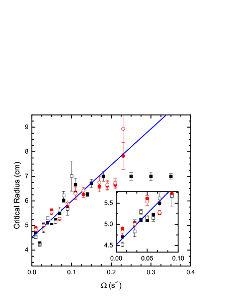
Figure 2: (color online) Comparison of the measured critical radius as a function of rotation rate for outer radii of 7 cm (black squares) and 9 cm (red circles). The open symbols correspond to calculation of $r_{c}$ using a Herschel-Bulkley model, and the solid symbols correspond to calculating $r_{c}$ assuming a power-law fluid coexisting with a solid-like state.

Three important features are highlighted by this figure. First, the critical radius is roughly linear in the applied rotation rate. (The straight line in the figure is a guide to the eye.) Second, for rotation rates less than $0.15\ {\rm s^{-1}}$, changing the system size does not alter the location of the coexistence between the two regions. Once the critical radius is $r_{c}=7\ {\rm cm}$, in the $R=9\ {\rm cm}$ system, the critical radius continues to increase with rotation rate. Finally, the critical radius approaches $r=4.5\ {\rm cm}$ as $\Omega$ goes to zero. The fact that $r_{c}\rightarrow 4.5\ {\rm cm}$ as $\Omega\rightarrow 0\ {\rm s^{-1}}$ is the first evidence for the breakdown of the Herschel-Bulkley model, as discussed in Sec. III. As a further test of the behavior of $r_{c}$, we have considered two slower rates of strain: $1.0\times 10^{-3}\ {\rm s^{-1}}$ and $3.0\times 10^{-3}\ {\rm s^{-1}}$. Due to the finite lifetime of the bubbles, the results for the velocity profiles were noisier at these extremely slow rates of strain than the data studied in detail in this paper. However, these profiles clearly exhibited a $r_{c}$ that was close to but greater than $4.5\ {\rm cm}$, consistent with the results reported in Fig. 2.

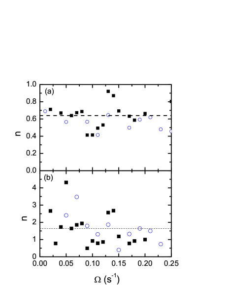
Figure 3: (color online) (a) The exponent $n$ obtained from fitting the velocity curves to a power-law fluid coexisting with a solid-like state versus the external rotation rate for $R=7\ {\rm cm}$ (black squares) and $R=9\ {\rm cm}$ (blue circles). (b) The exponent $n$ obtained from fitting the velocity curves to a Herschel-Bulkley model versus the external rotation rate for $R=7\ {\rm cm}$ (black squares) and $R=9\ {\rm cm}$ (blue circles).

As discussed, the exponent $n$ in both the Herschel-Bulkley model and the power-law model has physical significance. Figure 3 summarizes the values of $n$ obtained in the various fits to the velocity profiles. Figure 3a is the results for the power-law model, with the $R=7\ {\rm cm}$ and $R=9\ {\rm cm}$ indicated by squares and circles, respectively. Figure 3b is the results for the Herschel-Bulkley model. The dashed line in each figure represents the median value for the exponents. There are two striking features in Fig. 3. First, neither fit provides a completely consistent value for $n$. However, the variation in the fits for the power-law model is smaller than the case of the Herschel-Bulkley model. Second, for the power-law fits, one consistently finds $n<1$, but for the Herschel-Bulkley model, one consistently finds $n>1$ (though there are some isolated cases for which $n<1$).

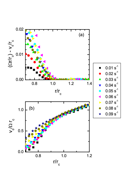
Figure 4: (color online) (a) Plot of the scaled velocity profiles $\tilde{v}=(\Omega r/r_{c})-v_{\theta}/r_{c}$ versus $r/r_{c}$. (b) Plot of $v_{\theta}/\Omega r_{c}$ versus $r/r_{c}$. Rates of strain are indicated in the legend.

As the combination of Figs. 2 and 3 effectively rule out a Herschel-Bulkley model, it is necessary to further probe the applicability of the power-law model. This allows us to confirm whether or not the transition is truly discontinuous in the rate of strain and to look a transition from continuum to discrete flow. One approach is to consider the scaling of the velocity profiles. In this regard, there are two different scalings that are particularly useful. These are presented in Fig. 4, and these represent the central measurement of both the discontinuity in the transition and the transition from continuum to discrete flow. First, it is useful to directly test for the existence of a consistent critical rate of strain in the context of the power-law model. To do this, we follow the scaling arguments presented in Ref. Rodts et al. (2005). Because we are rotating the outer cylinder, we first subtract out the rigid body rotation. This gives a new transformed velocity: $\tilde{v}=(\Omega r/r_{c})-v_{\theta}/r_{c}$. In this form, $\tilde{v}=0$ at $r=r_{c}$. Therefore, rewriting the rate of strain in the form $\dot{\gamma}(r)=r\frac{d}{dr}\frac{v_{\theta}(r)}{r}=\frac{dv_{\theta}}{dr}-\frac{v_{\theta}}{r}$, we see that the slope of $\tilde{v}$ at $r=r_{c}$ is the critical rate of strain $\dot{\gamma}_{c}$. Therefore, if there is a single $\dot{\gamma}_{c}$ for the material, then $\tilde{v}$ as a function of $r/r_{c}$ will collapse onto a single curve.

Figure 4a presents $\tilde{v}$ as a function of $r/r_{c}$. This illustrates two features. First, for sufficiently high rates of strain, the data suggests a single value of $\dot{\gamma}_{c}$. However, the scaling breaks down below a critical value of the external rotation rate. Second, this form of the velocity highlights the discontinuity in the slope at the critical radius.

Given the apparent dependence of $\dot{\gamma}_{c}$ on $\Omega$ for slow rates of strain, it is useful to consider an alternative scaling of the data, given in Fig. 4b. Here we plot $v_{\theta}/\Omega r_{c}$ as a function of $r/r_{c}$. For this case, we do not subtract the rigid body behavior, which is apparent as the linear regime for $r/r_{c}>1$. This was done to confirm the consistent rigid body behavior for all rotation rates. This scaling allows us to focus on the data for the slowest rotation rates, which did not scale in Fig. 4a. In this case, we observe a collapse of the data for slow rates of strain, indicating a dependence of $\dot{\gamma}_{c}$ on $\Omega$.

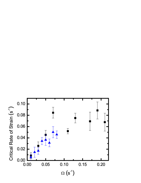
Figure 5: (color online) Critical rate of strain as a function of external rotation rate for $R=7\ {\rm cm}$ (blue triangles) and $R=9\ {\rm cm}$ (black squares).

The final measurement of the discrete/continuum flow transition is the direct measurement of $\dot{\gamma}_{c}$ as a function of $\Omega$. This is plotted in Fig. 5. In this case, we fit the data for $\tilde{v}$ near $r_{c}$. Two features of are illustrated by the data. First, for rotation rates below $\Omega=0.07\pm 0.02\ {\rm s^{-1}}$, the critical rates of strain are dependent on the external rotation rate, but independent of the system size. Interestingly, the behavior is consistent with a linear dependence on $\Omega$. This is strong evidence for the break down of any continuum description of the flow. Second, we observe a cross over to a regime in which $\dot{\gamma}_{c}$ is independent of $\Omega$. This occurs for value of the external rotation above $\Omega=0.07\pm 0.02\ {\rm s^{-1}}$ and is consistent with the scaling of $\tilde{v}$ presented in Fig. 4a. From this data, we find $\dot{\gamma}_{c}=0.07\pm 0.01\ {\rm s^{-1}}$, where the error represents the standard deviation of the measured values of the critical rate of strain, for our bubble raft.

Figure 6: Probability distribution of measuring a particular value of $r_{c}$ based on averaging the velocity over finite time intervals. Four different time intervals are illustrated for a rotation rate of $0.07\ {\rm s^{-1}}$ with $R=7\ {\rm cm}$. The time intervals and mean for each distribution are indicated in the figure.

Figure 7: Illustration of the convergence of the measured value of $r_{c}$ as a function of the time interval over which the average velocity is computed is increased.

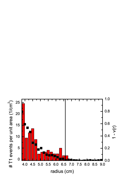
Figure 8: (color online) The T1 event rate for $R=9\ {\rm cm}$ and $\Omega=0.11\ {\rm s^{-1}}$ is shown as a function of $r$ (red histogram, left hand axis). This is compared to $1-v(r)$, where $v(r)=v_{\theta}(r)/\Omega r$ is the scaled velocity (black points, plotted against the right hand axis).

Given the possible breakdown of the continuum approximation, it is worth testing the short time behavior and determining the approach to steady state flow. This was done by considering a range of time intervals over which to compute the average bubble displacements, and the corresponding average velocity profiles. For short enough time intervals, we were able to compute a histogram of the probability distribution for $r_{c}$. Here, the probability distribution is computed as follows. For each independent time interval, an average velocity profile is computed. As reported in Ref. Dennin (2004), these profiles tend to be highly nonlinear, but there is a well-defined radius at which the profile deviates from a rigid body rotation. This point is taken as the critical radius for that realization of the velocity profile. This is computed for each independent segment of data from a single run, and the probability distribution is generated from this set of data.

Figure 6 presents the probability distribution for the case of $\Omega=0.07\ {\rm s^{-1}}$, and for four different time intervals used to compute the velocity profiles. As expected, the longer the time interval, the narrower the distribution. However, even for relatively short time intervals, the full width of the distribution is only on the order of $1\ {\rm cm}$, or about $3\ {\rm bubbles}$. As one increases the averaging time, the mean of the distribution remains constant to within 1 %. Another way of considering the approach to steady state is illustrated in Fig. 7. This shows the computed critical radius for different sets of data using a fixed time interval. The plot illustrates that for time intervals greater than 50 s, the computed value of $r_{c}$ does not change and that different measurements of $r_{c}$ give the same value. (Due to the length of the run, there are two points for the $\Delta t=60\ {\rm s}$ data, but one point for each of the larger values of $\Delta t$.)

A final question of interest is the spatial distribution of the T1 events and the correlation between the velocity profile and the T1 events. This is shown in Fig. 8 for $\Omega=0.11\ {\rm s^{-1}}$ and $R=9\ {\rm cm}$. Plotted here is a histogram of the number of T1 events in each radial bin (normalized by the area of the bin). This is compared to a plot of $1-v(r)$. The velocity is plotted in this form to better correlate the T1 and velocity distributions. The solid line indicates the position of $r_{c}$. One observes that the distribution of T1 events is consistent with the measurements of the distribution of $r_{c}$ for short time averages. As expected, one observes T1 events for values of $r$ close to, but slightly greater than, $r_{c}$. However, there are no observed T1 events for $r$ sufficiently greater than $r_{c}$.

V Discussion

The main focus of the measurements in this paper is to test carefully two aspects of the transition from solid to fluid behavior in a slowly driven foam. First, whether or not the transition is continuous or discontinuous in the rate of strain. Second, whether or not there is a transition from a discrete to a continuum flow regime. We used two standard models of complex fluids to interpret the experimental results: the Herschel-Bulkley model and a power-law model with a critical rate of strain. First, we will discuss the evidence against the Herschel-Bulkley model.

As discussed in Sec. III, the initial evidence against the Herschel-Bulkley model is the fact that $r_{c}$ does not approach $r_{i}$ as $\Omega$ goes to zero (see Fig. 2). Additional evidence against the model is the results for $n$ presented in Fig. 3. The fact that we essentially always measure an $n>1$, in direct contrast to the measurements of the stress as a function of rate of strain, rules out the Herschel-Bulkley model. Finally, the scaling of the velocity in Fig. 4 that strongly suggests the existence of a discontinuity in the rate of strain is behavior that is not possible in the context of the Herschel-Bulkley model. One might be concerned that despite this evidence, one appears to be able to fit the data to the Herschel-Bulkley model (as in Fig. 1). However, given the discrete nature of the data, the apparent fit to the Herschel-Bulkley model is most likely a result of the non-physical values of $n$ that are obtained.

In contrast to the Herschel-Bulkley model, the fits to the power-law model, and the scaling in Fig. 4a, strongly support the applicability of the power-law model and the corresponding discontinuity in the rate of strain. Therefore, it is reasonable to state the the localized flow in the bubble raft is best described by a coexistence of a power-law fluid and a solid region, with a discontinuity in rate of strain at the coexistence point. This has important implications for the jamming transition, as it suggests the equivalent of a first order transition. Also, it raises the important question of the mechanism that determines the critical rate of strain. This will be the subject of future work. One promising direction is to use a parallel shear cell. In this case, one expects a uniform stress across the system, and the global rate of strain is set by the boundaries. This can be used to further test the nature of the critical rates of strain. For example, in this case, it was determined to be $\dot{\gamma}_{c}=0.07\pm 0.01\ {\rm s^{-1}}$.

An interesting open question is which features of the flow are determined by the details of the bubble raft. For example, how does $\dot{\gamma}_{c}$ depend on the specifics of the solution used to make the bubbles, the polydispersity, the bubble size, etc.. Likewise, we observed that the value of $n$ has potentially significant variation. For example, even though $n<1$ based on fits to the power-law model (Fig. 3), it did differ from some past measurements in bubble rafts Lauridsen et al. (2004). This difference is not surprising given that the details of the bubble rafts differed to some degree in terms of the exact nature of the bubble size distribution and the solutions used to make the bubbles.

The transition from a continuum regime to a discrete regime is confirmed by the results presented in Figs. 4 and 5. Based on the scaling arguments from Ref. Rodts et al. (2005), the data in Fig. 4a is consistent with a single continuum model based on a power-law fluid with a critical rate of strain for sufficiently high rotation rates. The breakdown of the scaling indicates the transition to the discrete regime. Directly plotting the critical rate of strain for each rotation rate and system size, we find that the transition between discrete and continuum behavior occurs at $\Omega=0.07\pm 0.02\ {\rm s^{-1}}$. By considering two system sizes, we were also able to establish that the behavior is not dependent on system size. Conversely, we observe that the systems we have considered are large enough to exhibit behavior consistent with a continuum limit.

It is useful to compare our measurement of the transition to discrete flow with the reported measurements in a three-dimensional foam. Using the results in Fig. 2 for the critical radius, a transition at $\Omega=0.07\pm 0.02\ {\rm s^{-1}}$ corresponds to a critical thickness for the flowing regime of approximately 10 bubbles. For comparison, the same transition is observed in three-dimensional bubbles for a thickness of 25 bubbles and a rotation rate of $0.3\ {\rm s^{-1}}$ Rodts et al. (2005). At this point, it would be useful to consider both two and three dimensional models that capture this discontinuity to determine the source of the differences in these measurements. It might be dimensionality, but given the small differences, it is more likely related to details of the bubbles, such as bubble size, polydispersity, and surfactant composition. As current simulations only predict continuous transitions, work is first needed to elucidate the mechanism for the discontinuous transition.

The existence of the discrete regime also has implications for the jamming transition paradigm. The jamming transition is proposed in terms of an externally applied stress. However, this stress is often applied to the system using a constant external rate of strain. The system is then assumed to pass through the jamming transition as the stress increases as a function of total strain. It is not clear how the jamming transition should be understood in the discrete regime where the fluid-solid transition does not appear to be well-described by continuum models. This will be an interesting direction for future studies.

Finally, it is worth commenting on the insights gained by consideration of the short time behavior of the system. We focused on measurements of $r_{c}$ as a function of the averaging time (as shown in Figs. 6 and 7). This was useful because it provided confirmation that our results represent the steady-state of the system. In addition, the comparison of $r_{c}$ and the spatial distribution of T1 events are very suggestive.

The direct measurement of the distribution of T1 events confirmed the solid-like behavior for $r>r_{c}$ in terms of the complete absence of T1 events in the bulk of that region (Fig. 8). However, the T1 events do extend beyond $r_{c}$ by a few bubble radii. This is consistent with the width of the distribution of $r_{c}$ values for sufficiently short time measurements (Fig. 6). As T1 events occur right near $r_{c}$ (the steady-state average value), this will generate short-time bubble motions that can extend up to a few bubble diameters beyond $r_{c}$. These bubble motions can generate deviations from rigid body motion. Therefore, the fluctuations in $r_{c}$ have an important connection with the statistics of the T1 events at the transition from the fluid-like to the solid-like behavior. It will be interesting in the future to compare this to other fluctuating transitions between regions with different types of flow such as those that have been observed in other complex fluids Salmon et al. (2003b); Lerouge et al. (2006).

VI Appendix

In this Appendix, we present some of the details of the derivation of the velocity profiles. The derivation of the profile for the power-law fluid is standard Bird et al. (1977). One combines the the general expression for the stress in a Couette geometry and the relation between the stress and the rate of strain:

$$\sigma(r)=C/r^{2}=\mu(\dot{\gamma}/\dot{\gamma}_{c})^{n},$$ (6)

and combining all the constants, this simplifies to

$$\dot{\gamma}=D/r^{2/n}.$$ (7)

Using the definition of $\dot{\gamma}$, one gets

$$\dot{\gamma}=r\frac{d}{dr}\frac{v_{\theta}(r)}{r}=D/r^{2/n},$$ (8)

which can be directly integrated to get (dividing by $\Omega$)

$$\frac{v_{\theta}(r)}{\Omega r}\equiv v(r)=\frac{A}{r^{2/n}}-B.$$ (9)

As given in Sec. III, the boundary conditions determine $A$ and $B$ in terms of $n$, $r_{c}$, and $r_{i}$.

The derivation for the Herschel-Bulkley model follows along similar lines, only now it is useful to explicitly write out the constant in the stress relation:

$$\sigma(r)=C/r^{2}=\sigma(r_{i})r^{2}_{i}/r^{2}=\tau_{0}r^{2}_{c}/r^{2}.$$ (10)

Notice, that there are two equivalent ways to write the constant because it is based on the equivalence of torques in the radial direction Bird et al. (1977). Again, we equate this expression for the stress with the constitutive relation.

$$\tau_{0}r^{2}_{c}/r^{2}=\tau_{0}+\mu\dot{\gamma}^{n}.$$ (11)

This gives

$$\dot{\gamma}=(\tau_{0}/\mu)^{1/n}[r^{2}_{c}/r^{2}-1]^{1/n}.$$ (12)

In this case, integration does not result in an analytic expression, instead we get

$$\frac{v_{\theta}}{r}=\Big{(}\frac{\tau_{0}}{\mu}\Big{)}^{1/n}\int_{r_{i}}^{r}\frac{1}{\rho}\Big{(}\Big{(}\frac{r_{c}}{\rho}\Big{)}^{2}-1\Big{)}^{1/n}d\,\rho+C.$$ (13)

Here the constant $C=0$ because $v_{\theta}/r=0$ at $r=r_{i}$. Requiring solid body rotation $v_{\theta}=\Omega r$ at $r=r_{c}$ gives

$$\frac{v_{\theta}(r_{c})}{\Omega r_{c}}=1=\Big{(}\frac{\tau_{0}}{\mu}\Big{)}^{1/n}\int_{r_{i}}^{r_{c}}\frac{1}{\rho}\Big{(}\Big{(}\frac{r_{c}}{\rho}\Big{)}^{2}-1\Big{)}^{1/n}d\,\rho.$$ (14)

Therefore, converting to $v(r)\equiv v_{\theta}(r)/(\Omega r)$,

$$v(r)=\frac{1}{N}\int_{r_{i}}^{r}\frac{1}{\rho}\Big{(}\Big{(}\frac{r_{c}}{\rho}\Big{)}^{2}-1\Big{)}^{1/n}d\,\rho$$ (15)

where

$$N=\int_{r_{i}}^{r_{c}}\frac{1}{\rho}\Big{(}\Big{(}\frac{r_{c}}{\rho}\Big{)}^{2}-1\Big{)}^{1/n}d\,\rho.$$

This is a useful form for numerically fitting the data by approximating the integral.

References

- (1) Various books cover both the modelling and experimental measurement of yield stress materials, and complex fluids in general. Two examples are R. B. Bird, R. C. Armstrong, and O. Hassage, Dynamics of Polymer Liquids (Wiley, New York, 1977) and C. Macosko, Rheology Principles, Measurements, and Applications (VCH Publishers, New York, 1994).
- Debrégeas et al. (2001) G. Debrégeas, H. Tabuteau, and J. M. di Meglio, Phys. Rev. Lett. 87, 178305 (2001).
- Lauridsen et al. (2004) J. Lauridsen, G. Chanan, and M. Dennin, Phys. Rev. Lett. 93, 018303 (2004).
- Coussot et al. (2002) P. Coussot, J. S. Raynaud, F. Bertrand, P. Moucheront, J. P. Guilbaud, H. T. Huynh, S. Jarny, and D. Lesueur, Phys. Rev. Lett. 88, 218301 (2002).
- Salmon et al. (2003a) J.-B. Salmon, A. Colin, S. Manneville, and F. Molino, Phys. Rev. Lett. 90, 228303 (2003a).
- Lerouge et al. (2006) S. Lerouge, M. Argentina, and J. P. Decruppe, Phys. Rev. Lett. 96, 088301 (pages 4) (2006).
- Salmon et al. (2003b) J.-B. Salmon, S. Manneville, and A. Colin, Phys. Rev. E 68, 051504 (pages 10) (2003b).
- Salmon et al. (2003c) J.-B. Salmon, S. Manneville, and A. Colin, Phys. Rev. E 68, 051503 (pages 12) (2003c).
- Howell et al. (1999) D. Howell, R. P. Behringer, and C. Veje, Phys. Rev. Lett. 82, 5241 (1999).
- Losert et al. (2000) W. Losert, L. Bocquet, T. C. Lubensky, and J. P. Gollub, Phys. Rev. Lett. 85, 1428 (2000).
- Mueth et al. (2000) D. M. Mueth, G. F. Debregeas, G. S. Karczmar, P. J. Eng, S. R. Nagel, and H. M. Jaeger, Nature 406, 385 (2000).
- Huang et al. (2005) N. Huang, G. Ovarlez, F. Bertrand, S. Rodts, P. Coussot, and D. Bonn, Phys. Rev. Lett. 94, 028301 (2005).
- Gopal and Durian (1999) A. D. Gopal and D. J. Durian, J. Colloid. Interf. Sci. 213, 169 (1999).
- Lauridsen et al. (2002) J. Lauridsen, M. Twardos, and M. Dennin, Phys. Rev. Lett. 89, 098303 (2002).
- Rouyer et al. (2003) F. Rouyer, S. Cohen-Addad, M. Vignes-Adler, and R. Höhler, Phys. Rev. E 67, 021405 (2003).
- Rodts et al. (2005) S. Rodts, , J. C. Baudez, and P. Coussot, Europhysics Letters 69, 636 (2005).
- Liu and Nagel (1998) A. J. Liu and S. R. Nagel, Nature 396, 21 (1998).
- Liu and Nagel (2001) A. J. Liu and S. R. Nagel, eds., Jamming and Rheology (Taylor and Francis Group, 2001).
- Wang et al. (2006) Y. Wang, K. Krishan, and M. Dennin, Phys. Rev. E 73, 031401 (2006).
- Weaire et al. (2006) D. Weaire, E. Janiaud, and S. Hutzler, Two dimensional foam rheology with viscous drag (2006), URL http://www.citebase.org/cgi-bin/citations?id=oai:arXiv.org:co%nd-mat/0602021.
- Kabla and Debrégeas (2003) A. Kabla and G. Debrégeas, Phys. Rev. Lett. 90, 258303 (2003).
- Varnik et al. (2003) F. Varnik, L. Bocquet, J.-L. Barrat, and L. Berthier, Phys. Rev. Lett. 90, 095702 (2003).
- Xu et al. (2005a) N. Xu, C. S. O’Hern, and L. Kondic, Phys. Rev. Lett. 94, 016001 (2005a).
- Xu et al. (2005b) N. Xu, C. S. O’Hern, and L. Kondic, Phys. Rev. E 72, 041504 (2005b).
- Bragg and Lomer (1949) L. Bragg and W. M. Lomer, Proc. R. Soc. London, Ser. A 196, 171 (1949).
- Argon and Kuo (1979) A. S. Argon and H. Y. Kuo, Mat. Sci. and Eng. 39, 101 (1979).
- Ghaskadvi and Dennin (1998) R. S. Ghaskadvi and M. Dennin, Rev. Sci. Instr. 69, 3568 (1998).
- Bird et al. (1977) R. B. Bird, R. C. Armstrong, and O. Hassager, Dynamics of Polymer Liquids (Wiley, New York, 1977).
- Pratt and Dennin (2003) E. Pratt and M. Dennin, Phys. Rev. E 67, 051402 (2003).
- Dennin (2004) M. Dennin, Phys. Rev. E 70, 041406 (2004).